
CLTS-Net: A More Accurate and Universal Method for the Long-Term Prediction of Significant Wave Height


Abstract
:1. Introduction
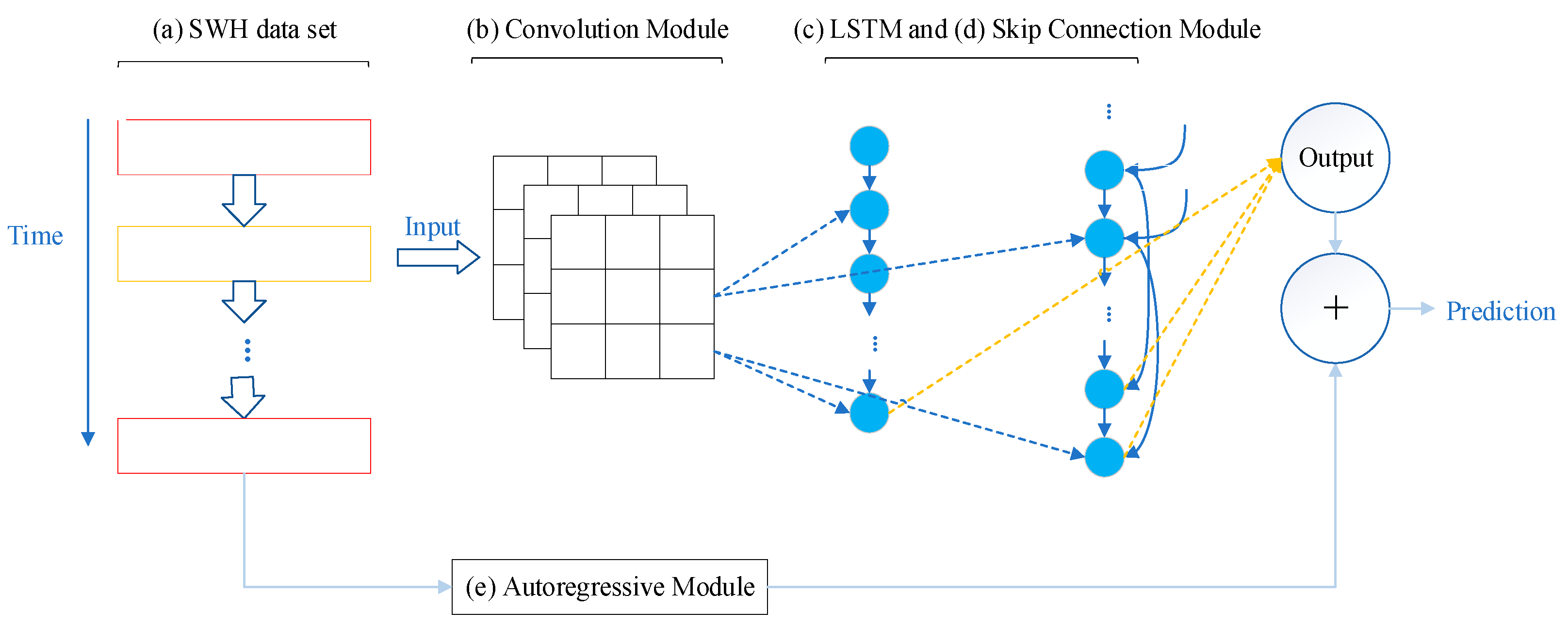
2. Proposed Method
2.1. Convolutional Neural Network Module
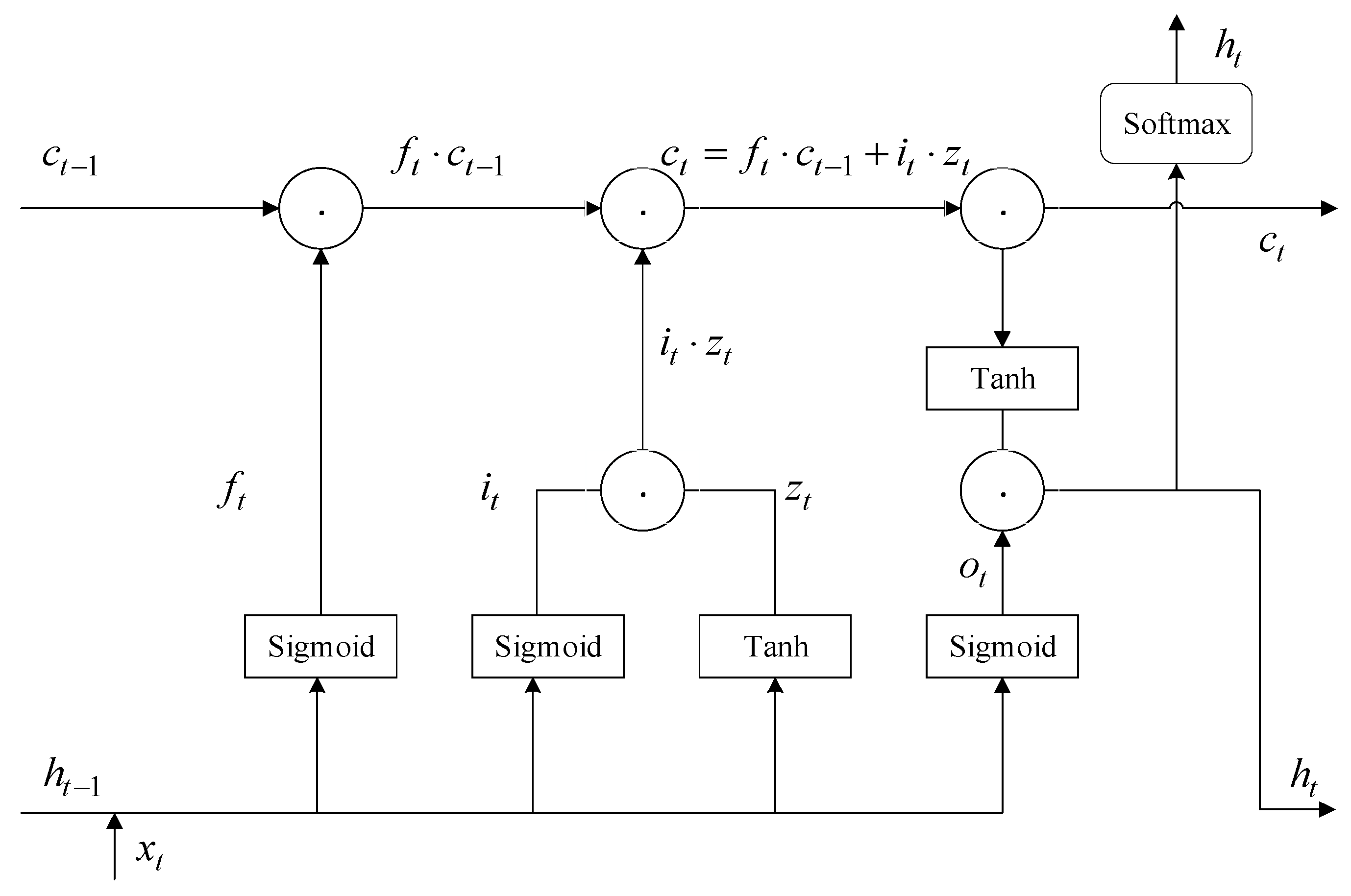
2.2. Long Short-Term Memory Module
2.3. Skip Connection Module
2.4. Autoregressive Module
3. Evaluation
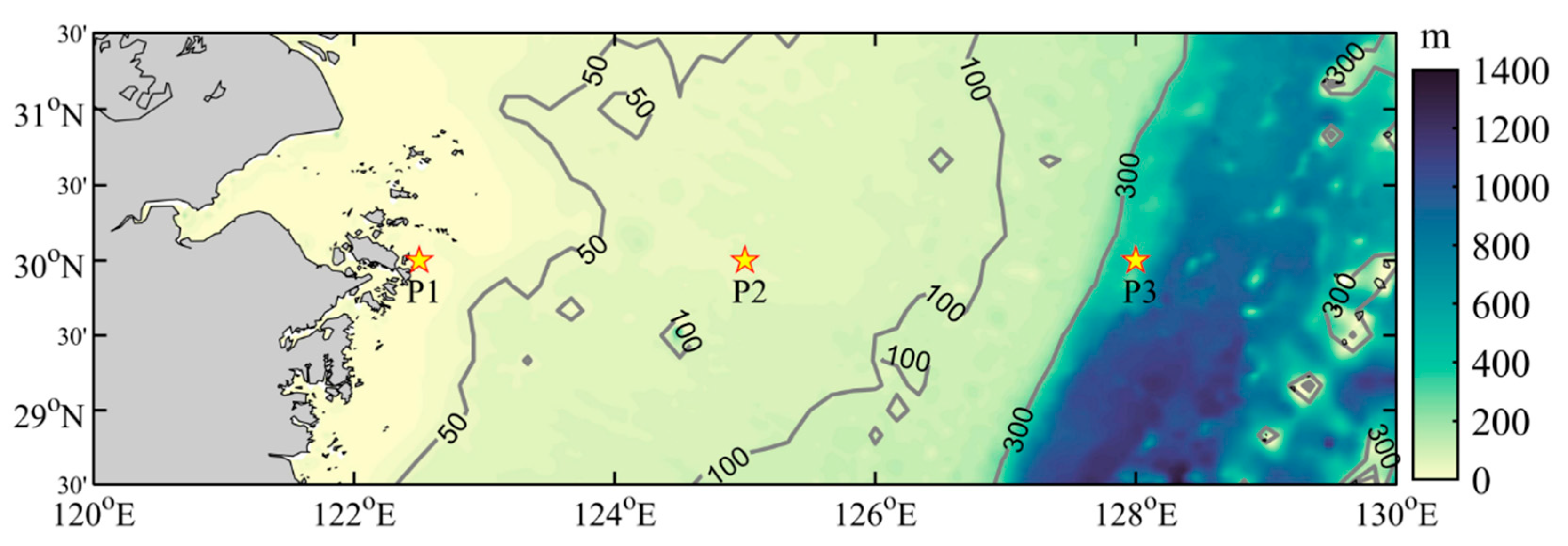
3.1. Dataset
3.2. Methods for Comparison
3.3. Metrics
3.4. Experimental Details
4. Results
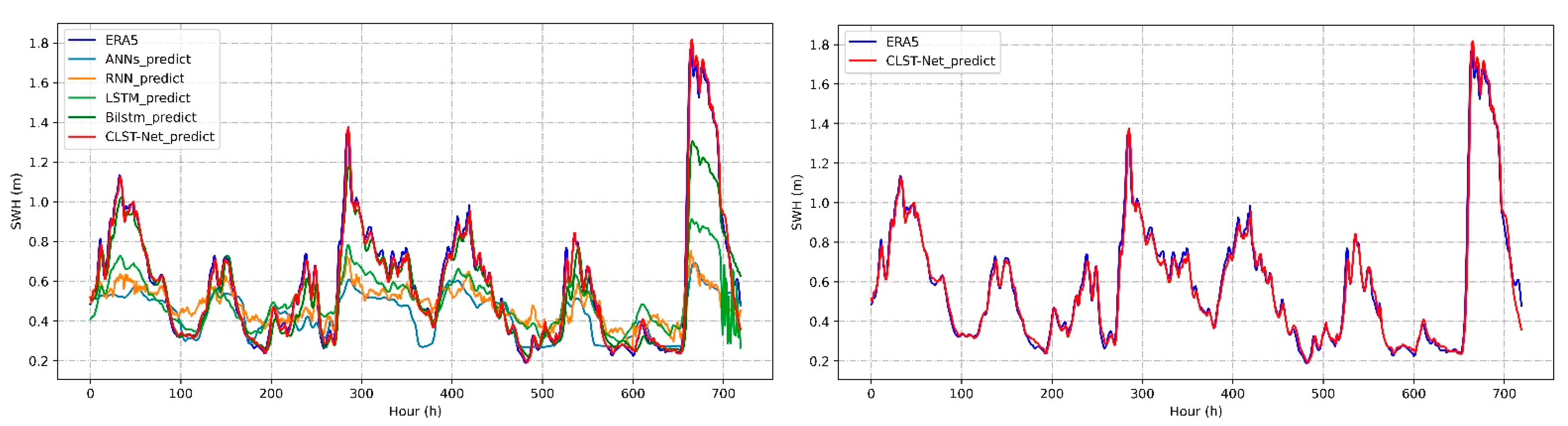
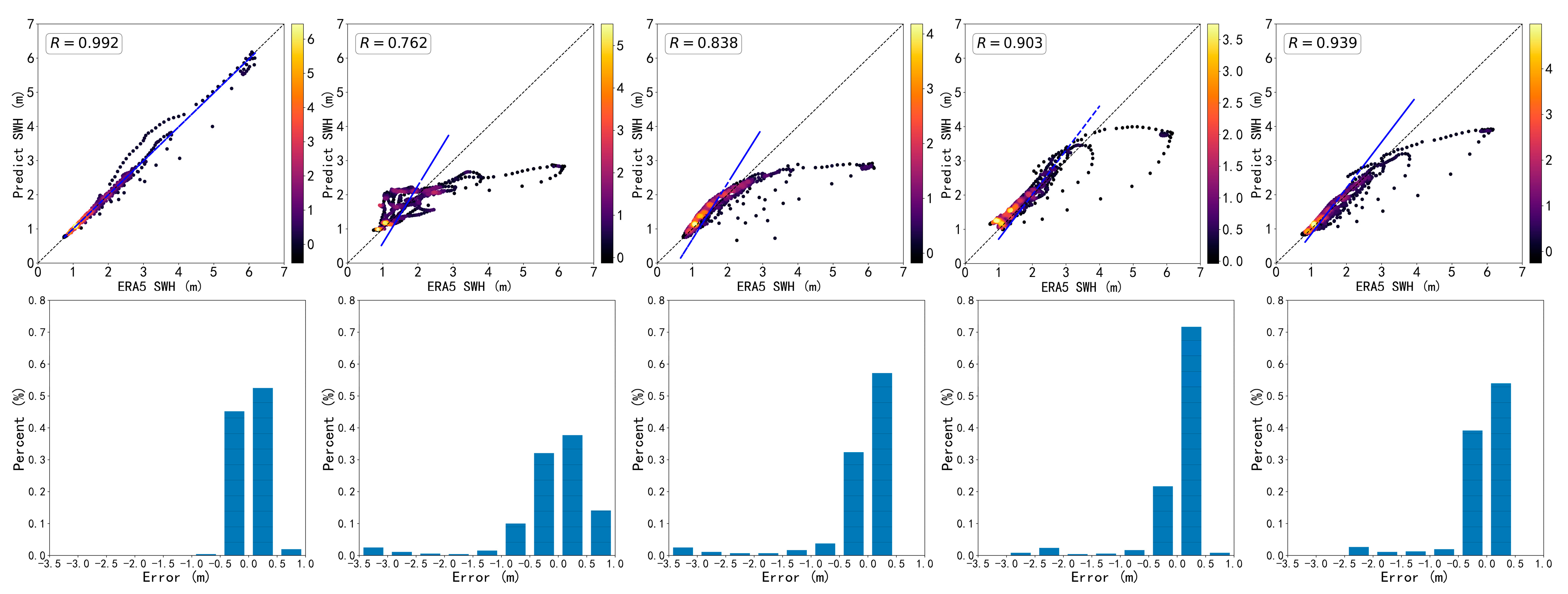
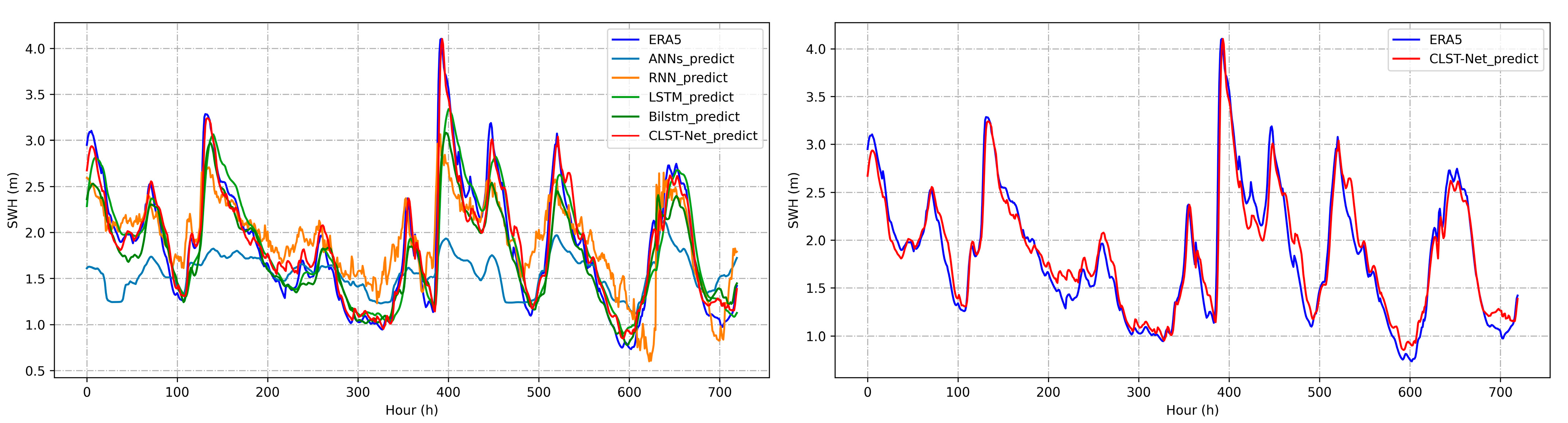
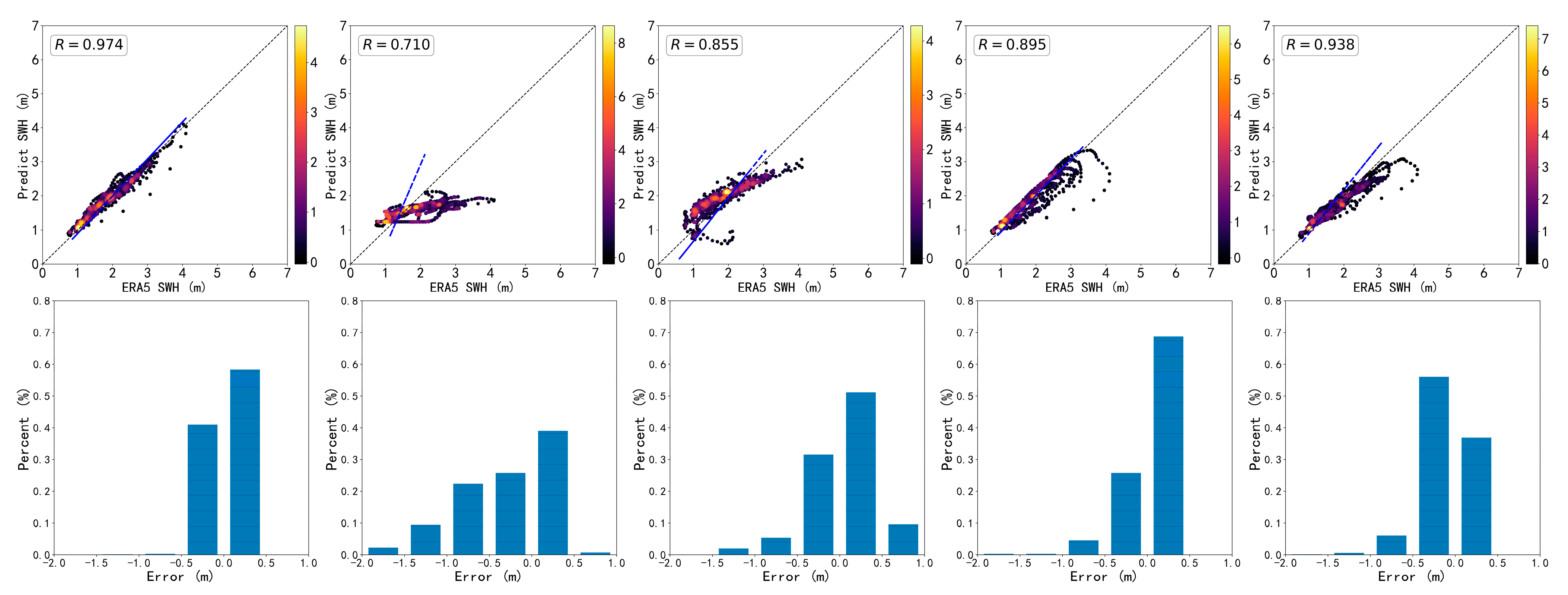
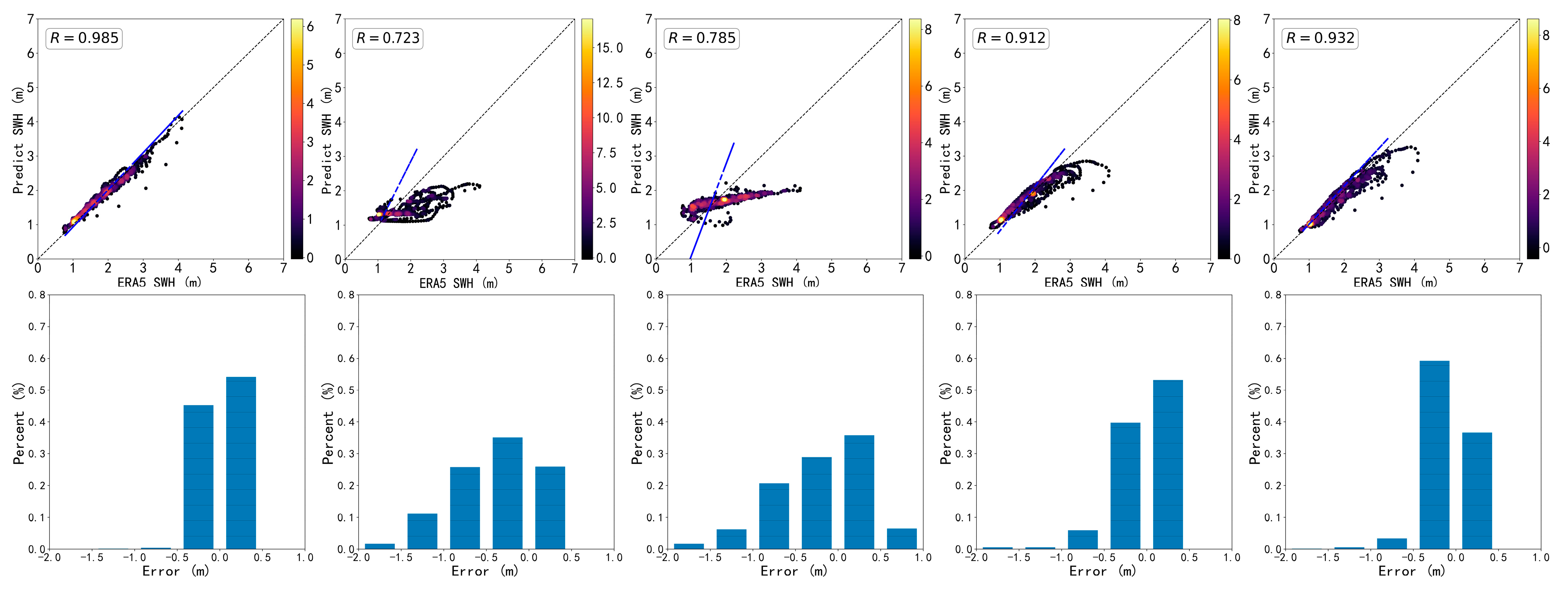
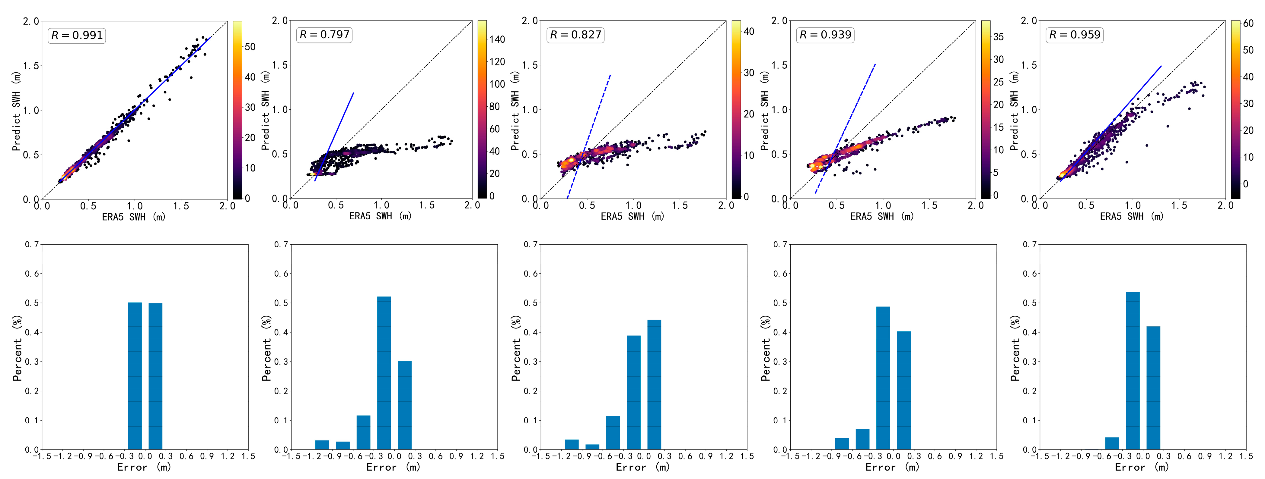
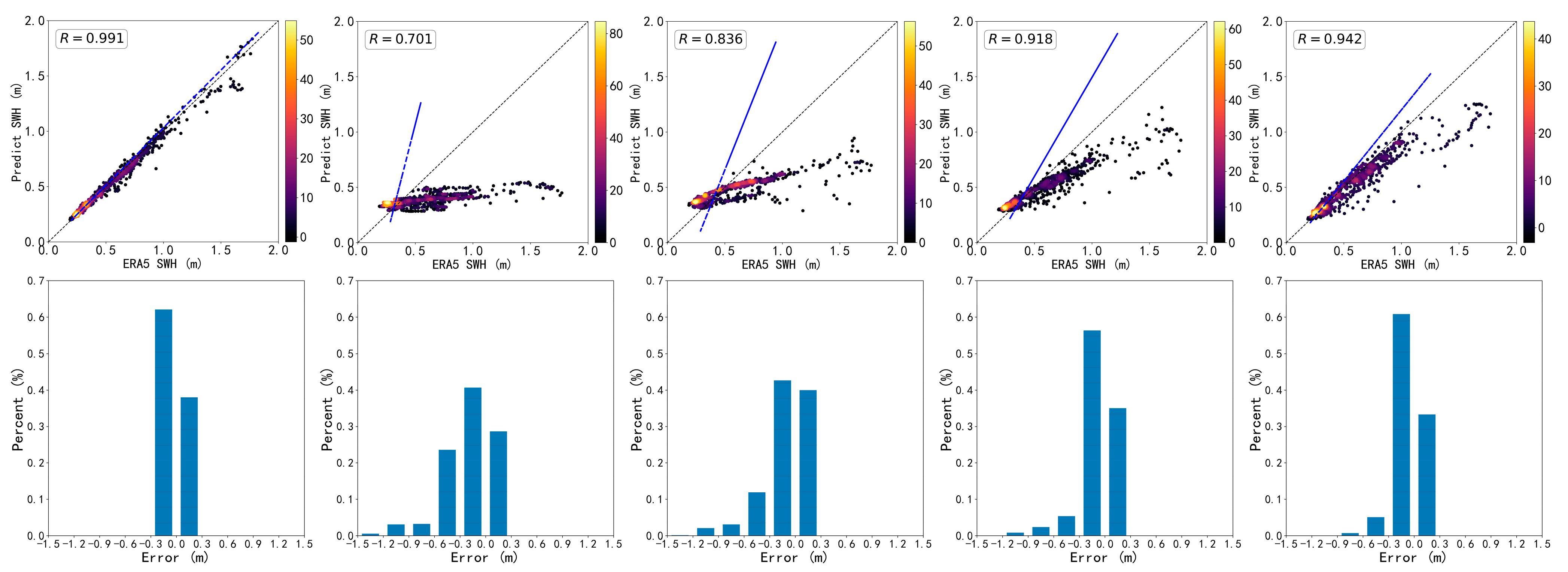
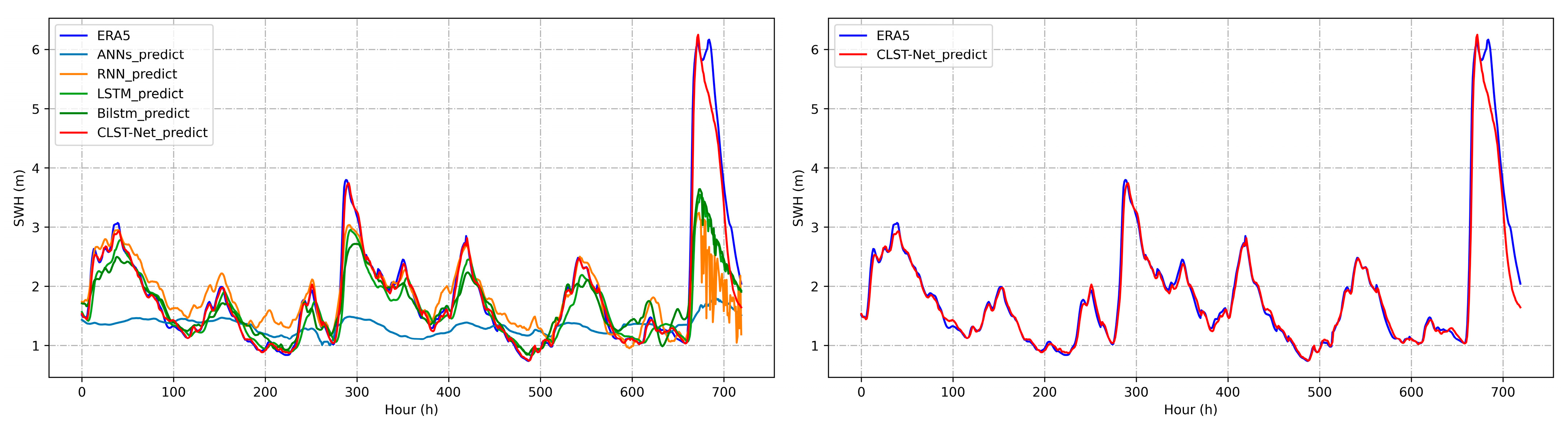
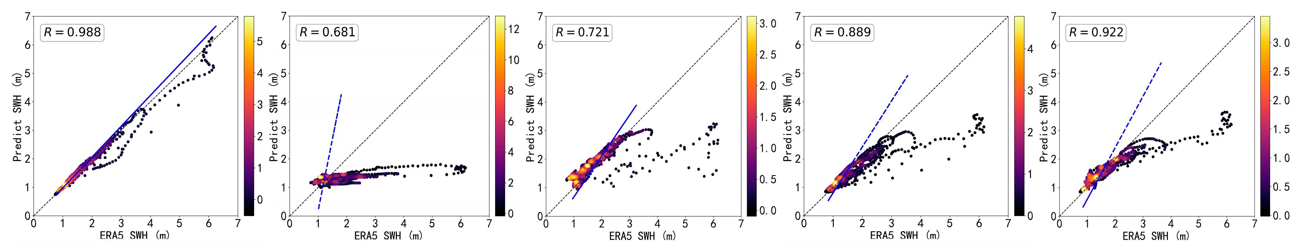
4.1. SWH Forecast Performance at P1
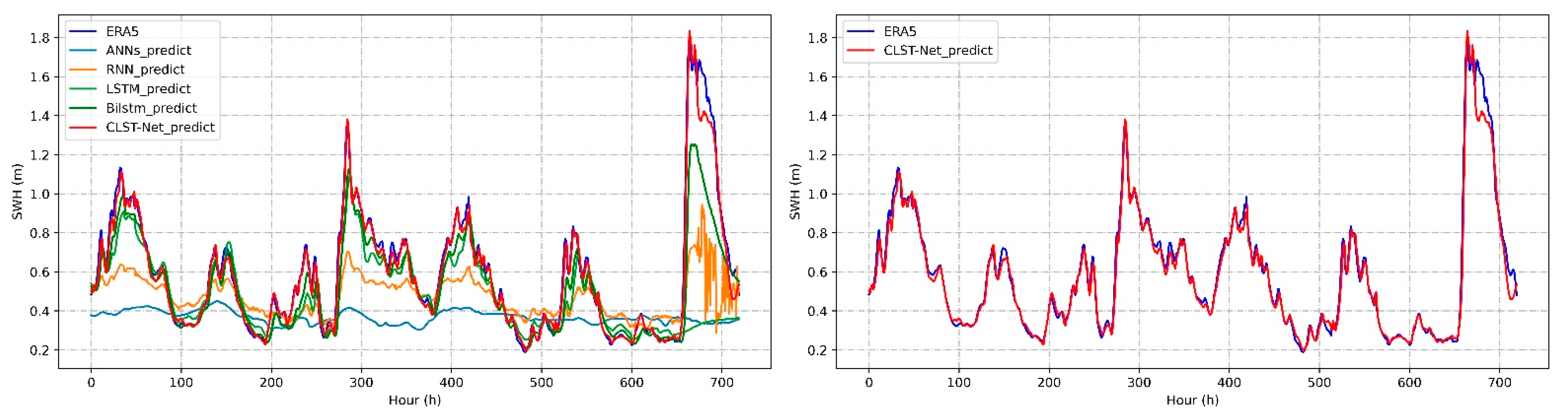
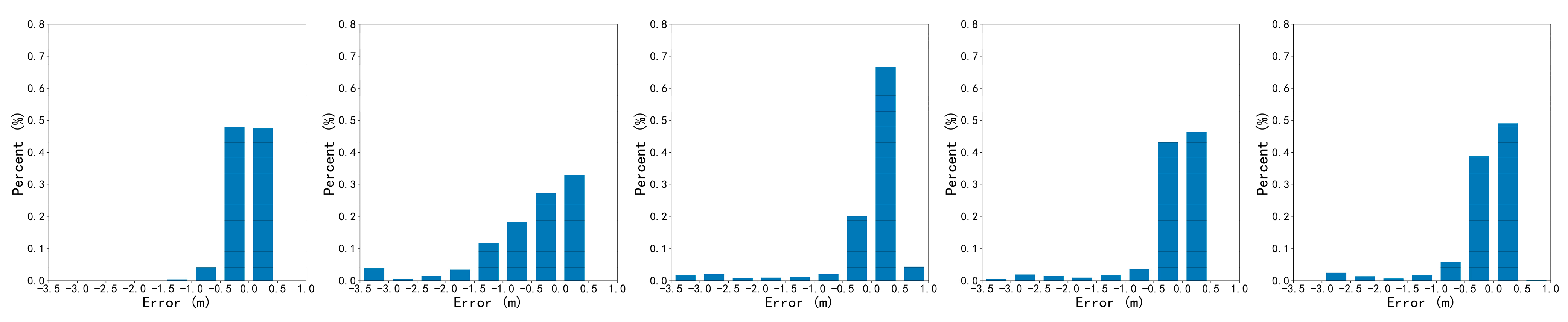
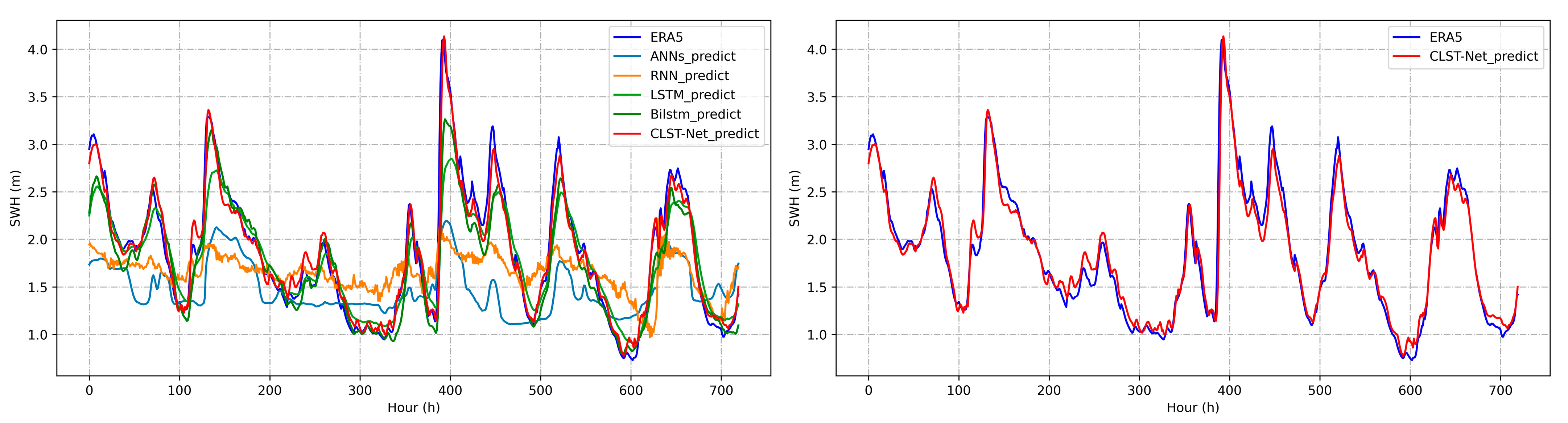
4.2. SWH Forecast Performance at P2
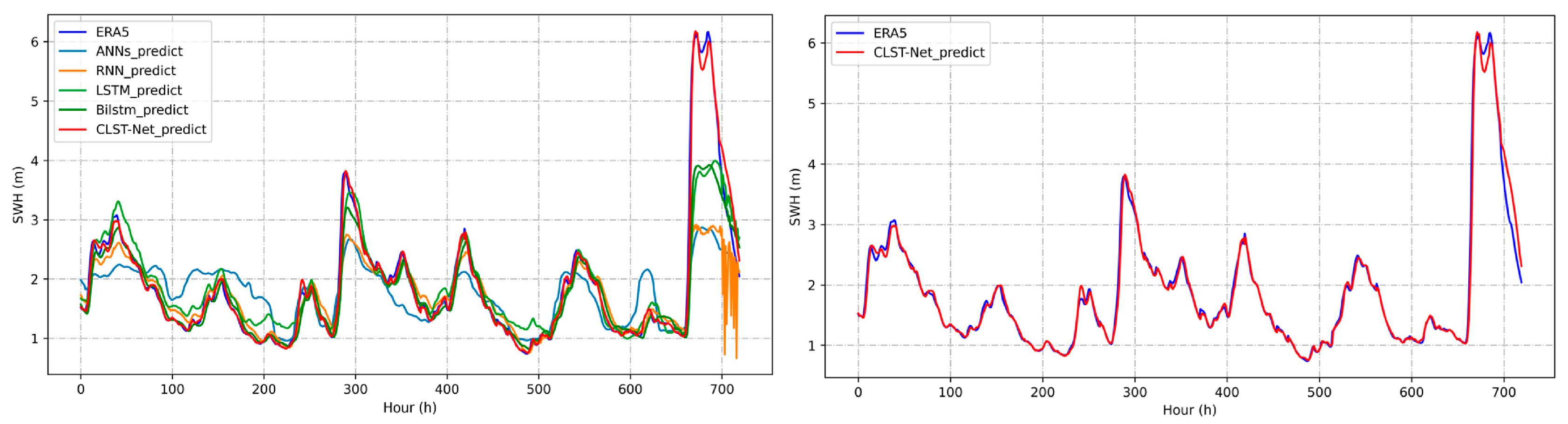
4.3. SWH Forecast Performance at P3
5. Conclusions
Author Contributions
Funding
Institutional Review Board Statement
Informed Consent Statement
Data Availability Statement
Acknowledgments
Conflicts of Interest
References
- Gao, S.; Huang, J.; Li, Y.; Liu, G.; Bi, F.; Bai, Z. A forecasting model for wave heights based on a long short-term memory neural network. Acta Oceanol. Sin. 2021, 40, 62–69. [Google Scholar] [CrossRef]
- Young, I.R.; Ribal, A. Multiplatform evaluation of global trends in wind speed and wave height. Science 2019, 364, 548–552. [Google Scholar] [CrossRef] [PubMed]
- Gopinath, D.; Dwarakish, G. Wave Prediction Using Neural Networks at New Mangalore Port along West Coast of India. Aquat. Procedia 2015, 4, 143–150. [Google Scholar] [CrossRef]
- Fazeres-Ferradosa, T.; Rosa-Santos, P.; Taveira-Pinto, F.; Vanem, E.; Carvalho, H.; Correia, J.A.F.D.O. Editorial: Advanced research on offshore structures and foundation design: Part 1. Proc. Inst. Civ. Eng. Marit. Eng. 2019, 172, 118–123. [Google Scholar] [CrossRef]
- Vanem, E.; Fazeres-Ferradosa, T.; Rosa-Santos, P.; Taveira-Pinto, F. Statistical description and modelling of extreme ocean wave conditions. In Proceedings of the Institution of Civil Engineers—Maritime Engineering, London, UK, 19 December 2019; Thomas Telford Ltd.: London, UK, 2019; Volume 172, pp. 124–132. [Google Scholar]
- Umesh, P.; Swain, J. Inter-comparisons of SWAN hindcasts using boundary conditions from WAM and WWIII for northwest and northeast coasts of India. Ocean Eng. 2018, 156, 523–549. [Google Scholar] [CrossRef]
- Swain, J.; Umesh, P.; Balchand, A. WAM and WAVEWATCH-III intercomparison studies in the North Indian Ocean using Oceansat-2 Scatterometer winds. J. Ocean Clim. Sci. Technol. Impacts 2019, 9, 2516019219866569. [Google Scholar] [CrossRef] [Green Version]
- Group, T.W. The WAM model—A third generation ocean wave prediction model. J. Phys. Oceanogr. 1988, 18, 1775–1810. [Google Scholar] [CrossRef] [Green Version]
- Li, N.; Cheung, K.F.; Cross, P. Numerical wave modeling for operational and survival analyses of wave energy converters at the US Navy Wave Energy Test Site in Hawaii. Renew. Energy 2020, 161, 240–256. [Google Scholar] [CrossRef]
- Kazeminezhad, M.H.; Siadatmousavi, S.M. Performance evaluation of WAVEWATCH III model in the Persian Gulf using different wind resources. Ocean Dyn. 2017, 67, 839–855. [Google Scholar] [CrossRef]
- Liu, Q.; Rogers, W.E.; Babanin, A.V.; Young, I.R.; Romero, L.; Zieger, S.; Qiao, F.; Guan, C. Observation-Based Source Terms in the Third-Generation Wave Model WAVEWATCH III: Updates and Verification. J. Phys. Oceanogr. 2019, 49, 489–517. [Google Scholar] [CrossRef]
- Lin, Y.; Dong, S.; Wang, Z.; Soares, C.G. Wave energy assessment in the China adjacent seas on the basis of a 20-year SWAN simulation with unstructured grids. Renew. Energy 2019, 136, 275–295. [Google Scholar] [CrossRef]
- Akpınar, A.; Bingölbali, B.; Van Vledder, G.P. Long-term analysis of wave power potential in the Black Sea, based on 31-year SWAN simulations. Ocean Eng. 2017, 130, 482–497. [Google Scholar] [CrossRef]
- Liang, B.; Gao, H.; Shao, Z. Characteristics of global waves based on the third-generation wave model SWAN. Mar. Struct. 2019, 64, 35–53. [Google Scholar] [CrossRef]
- Huang, W.; Dong, S. Improved short-term prediction of significant wave height by decomposing deterministic and stochastic components. Renew. Energy 2021, 177, 743–758. [Google Scholar] [CrossRef]
- Zhou, S.; Xie, W.; Lu, Y.; Wang, Y.; Zhou, Y.; Hui, N.; Dong, C. ConvLSTM-Based Wave Forecasts in the South and East China Seas. Front. Mar. Sci. 2021, 8, 740. [Google Scholar] [CrossRef]
- Makarynskyy, O.; Pires-Silva, A.A.; Makarynska, D.; Ventura-Soares, C. Artificial neural networks in wave predictions at the west coast of Portugal. Comput. Geosci. 2005, 31, 415–424. [Google Scholar] [CrossRef] [Green Version]
- Gopinath, D.I.; Dwarakish, G.S.; Systems, C. Real-time prediction of waves using neural networks trained by particle swarm optimization. Int. J. Ocean. Clim. Syst. 2016, 7, 70–79. [Google Scholar] [CrossRef] [Green Version]
- Deshmukh, A.N.; Deo, M.C.; Bhaskaran, P.K.; Nair, T.M.B.; Sandhya, K.G. Neural-Network-Based Data Assimilation to Improve Numerical Ocean Wave Forecast. IEEE J. Ocean. Eng. 2016, 41, 944–953. [Google Scholar] [CrossRef]
- Deo, M.; Jha, A.; Chaphekar, A.; Ravikant, K. Neural networks for wave forecasting. Ocean Eng. 2001, 28, 889–898. [Google Scholar] [CrossRef]
- Londhe, S.; Panchang, V. One-day wave forecasts based on artificial neural networks. J. Atmos. Ocean. Technol. 2006, 23, 1593–1603. [Google Scholar] [CrossRef] [Green Version]
- Peres, D.; Iuppa, C.; Cavallaro, L.; Cancelliere, A.; Foti, E. Significant wave height record extension by neural networks and reanalysis wind data. Ocean Model. 2015, 94, 128–140. [Google Scholar] [CrossRef]
- Ni, C.; Ma, X. An integrated long-short term memory algorithm for predicting polar westerlies wave height. Ocean Eng. 2020, 215, 107715. [Google Scholar] [CrossRef]
- Zaremba, W.; Sutskever, I.; Vinyals, O. Recurrent Neural Network Regularization. arXiv 2014, arXiv:1409.2329. [Google Scholar]
- Mandal, S.; Prabaharan, N. Ocean wave forecasting using recurrent neural networks. Ocean Eng. 2006, 33, 1401–1410. [Google Scholar] [CrossRef]
- Sadeghifar, T.; Motlagh, M.N.; Azad, M.T.; Mahdizadeh, M.M. Coastal Wave Height Prediction using Recurrent Neural Networks (RNNs) in the South Caspian Sea. Mar. Geodesy 2017, 40, 454–465. [Google Scholar] [CrossRef]
- Miky, Y.; Kaloop, M.R.; Elnabwy, M.T.; Baik, A.; Alshouny, A. A Recurrent-Cascade-Neural network- nonlinear autoregressive networks with exogenous inputs (NARX) approach for long-term time-series prediction of wave height based on wave characteristics measurements. Ocean Eng. 2021, 240, 109958. [Google Scholar] [CrossRef]
- Hochreiter, S.; Schmidhuber, J.J. Long short-term memory. Neural Comput. 1997, 9, 1735–1780. [Google Scholar] [CrossRef] [PubMed]
- Fan, S.; Xiao, N.; Dong, S. A novel model to predict significant wave height based on long short-term memory network. Ocean Eng. 2020, 205, 107298. [Google Scholar] [CrossRef]
- Zhang, X.; Li, Y.; Gao, S.; Ren, P. Ocean Wave Height Series Prediction with Numerical Long Short-Term Memory. J. Mar. Sci. Eng. 2021, 9, 514. [Google Scholar] [CrossRef]
- Raj, N.; Brown, J. An EEMD-BiLSTM Algorithm Integrated with Boruta Random Forest Optimiser for Significant Wave Height Forecasting along Coastal Areas of Queensland, Australia. Remote. Sens. 2021, 13, 1456. [Google Scholar] [CrossRef]
- Goodfellow, I.; Bengio, Y.; Courville, A. Deep Learning; MIT Press: Cambridge, MA, USA, 2016. [Google Scholar]
- He, K.M.; Zhang, X.Y.; Ren, S.Q.; Sun, J. Deep residual learning for image recognition. In Proceedings of the IEEE Conference on Computer Vision and Pattern Recognition (CVPR), Seattle, WA, USA, 27–30 June 2016; pp. 770–778. [Google Scholar] [CrossRef] [Green Version]


| Metrics | Method | 24 h | 48 h | 72 h |
|---|---|---|---|---|
| RMSE | ANN | 0.2881 | 0.3520 | 0.4102 |
| RNN | 0.2750 | 0.2668 | 0.3199 | |
| LSTM | 0.2182 | 0.2044 | 0.3124 | |
| Bi-LSTM | 0.1102 | 0.1413 | 0.3076 | |
| CLTS-Net | 0.0424 | 0.0465 | 0.2008 | |
| MAE | ANN | 0.1864 | 0.2470 | 0.2837 |
| RNN | 0.1821 | 0.1796 | 0.1876 | |
| LSTM | 0.1509 | 0.1309 | 0.1685 | |
| Bi-LSTM | 0.0628 | 0.0817 | 0.1486 | |
| CLTS-Net | 0.0270 | 0.0280 | 0.0706 | |
| MAPE | ANN | 0.2505 | 0.3472 | 0.3773 |
| RNN | 0.2802 | 0.2750 | 0.2631 | |
| LSTM | 0.2426 | 0.1924 | 0.2234 | |
| Bi-LSTM | 0.0927 | 0.1159 | 0.1818 | |
| CLTS-Net | 0.0469 | 0.0447 | 0.0764 | |
| R | ANN | 0.7966 | 0.7010 | 0.2218 |
| RNN | 0.8274 | 0.8357 | 0.4559 | |
| LSTM | 0.9385 | 0.9180 | 0.4772 | |
| Bi-LSTM | 0.9593 | 0.9420 | 0.5017 | |
| CLTS-Net | 0.9913 | 0.9911 | 0.8054 |
| Metrics | Method | 24 h | 48 h | 72 h |
|---|---|---|---|---|
| RMSE | ANN | 0.7611 | 1.0941 | 1.1397 |
| RNN | 0.6852 | 0.7564 | 1.1105 | |
| LSTM | 0.5001 | 0.6299 | 1.0183 | |
| Bi-LSTM | 0.4563 | 0.6117 | 0.9827 | |
| CLTS-Net | 0.1314 | 0.1824 | 0.7740 | |
| MAE | ANN | 0.4589 | 0.6798 | 0.7015 |
| RNN | 0.3162 | 0.3819 | 0.6290 | |
| LSTM | 0.2673 | 0.2972 | 0.3790 | |
| Bi-LSTM | 0.2045 | 0.3091 | 0.3801 | |
| CLTS-Net | 0.0618 | 0.0868 | 0.2444 | |
| MAPE | ANN | 0.2271 | 0.2879 | 0.3038 |
| RNN | 0.1252 | 0.1910 | 0.2564 | |
| LSTM | 0.1372 | 0.1151 | 0.1233 | |
| Bi-LSTM | 0.0823 | 0.1324 | 0.1310 | |
| CLTS-Net | 0.0276 | 0.0389 | 0.0757 | |
| R | ANN | 0.7616 | 0.6814 | 0.2157 |
| RNN | 0.8381 | 0.7214 | 0.4139 | |
| LSTM | 0.9026 | 0.8886 | 0.3993 | |
| Bi-LSTM | 0.9387 | 0.9215 | 0.4495 | |
| CLTS-Net | 0.9921 | 0.9883 | 0.7107 |
| Metrics | Method | 24 h | 48 h | 72 h |
|---|---|---|---|---|
| RMSE | ANN | 0.6239 | 0.6415 | 0.7029 |
| RNN | 0.3792 | 0.5715 | 0.5917 | |
| LSTM | 0.3009 | 0.3092 | 0.5161 | |
| Bi-LSTM | 0.2868 | 0.2681 | 0.4990 | |
| CLTS-Net | 0.1647 | 0.1271 | 0.1283 | |
| MAE | ANN | 0.4676 | 0.5020 | 0.5319 |
| RNN | 0.3053 | 0.4470 | 0.4650 | |
| LSTM | 0.2098 | 0.2049 | 0.4058 | |
| Bi-LSTM | 0.1964 | 0.1772 | 0.3649 | |
| CLTS-Net | 0.1275 | 0.0914 | 0.0900 | |
| MAPE | ANN | 0.2341 | 0.2497 | 0.2745 |
| RNN | 0.1985 | 0.2418 | 0.2663 | |
| LSTM | 0.1151 | 0.1082 | 0.2350 | |
| Bi-LSTM | 0.0999 | 0.0889 | 0.1944 | |
| CLTS-Net | 0.0760 | 0.0524 | 0.0553 | |
| R | ANN | 0.7101 | 0.7234 | 0.3123 |
| RNN | 0.8552 | 0.7850 | 0.6260 | |
| LSTM | 0.8950 | 0.9117 | 0.6649 | |
| Bi-LSTM | 0.9377 | 0.9315 | 0.6971 | |
| CLTS-Net | 0.9736 | 0.9850 | 0.9844 |
Publisher’s Note: MDPI stays neutral with regard to jurisdictional claims in published maps and institutional affiliations. |
© 2021 by the authors. Licensee MDPI, Basel, Switzerland. This article is an open access article distributed under the terms and conditions of the Creative Commons Attribution (CC BY) license (https://creativecommons.org/licenses/by/4.0/).
Share and Cite
Li, S.; Hao, P.; Yu, C.; Wu, G. CLTS-Net: A More Accurate and Universal Method for the Long-Term Prediction of Significant Wave Height. J. Mar. Sci. Eng. 2021, 9, 1464. https://doi.org/10.3390/jmse9121464
Li S, Hao P, Yu C, Wu G. CLTS-Net: A More Accurate and Universal Method for the Long-Term Prediction of Significant Wave Height. Journal of Marine Science and Engineering. 2021; 9(12):1464. https://doi.org/10.3390/jmse9121464
Chicago/Turabian StyleLi, Shuang, Peng Hao, Chengcheng Yu, and Gengkun Wu. 2021. "CLTS-Net: A More Accurate and Universal Method for the Long-Term Prediction of Significant Wave Height" Journal of Marine Science and Engineering 9, no. 12: 1464. https://doi.org/10.3390/jmse9121464
APA StyleLi, S., Hao, P., Yu, C., & Wu, G. (2021). CLTS-Net: A More Accurate and Universal Method for the Long-Term Prediction of Significant Wave Height. Journal of Marine Science and Engineering, 9(12), 1464. https://doi.org/10.3390/jmse9121464