On the Non-Gaussianity of the Height of Sea Waves


Abstract
:1. Introduction
2. Dataset
3. Methodology
- (E1.)
- X is an ergodic stationary process.
- (E2.)
- The characteristic function of the one-dimensional marginal of X is analytic.
- (E3.)
- (E4.)
- The spectral density matrix of the process:at frequency 0 exists and is positive definite. In (1) the with are drawn at random in such a way that and are independent and identically distributed with an absolutely continuous distribution.
- (L1.)
- X is an ergodic stationary process.
- (L2.)
- (L3.)
- where and the are independent and identically distributed random variables with and
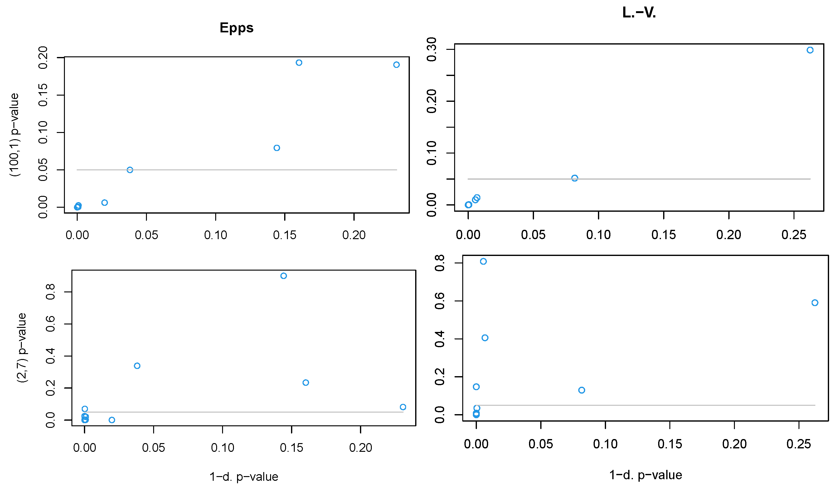
- Parameters (100,1) with the Lobato and Velasco test: The non-Gaussianity of the process is related to the third and/or fourth order moment of a small dimensional distribution of the original non-projected process.
- Parameters (2,7) with the Lobato and Velasco test: The non-Gaussianity of the process is related to the third and/or fourth order moment of the one-dimensional distribution of the projected process.
- Parameters (100,1) with the Epps test: The non-Gaussianity of the process is related in general to a small dimensional distribution of the original non-projected process.
- Parameters (2,7) with the Epps test: tThe non-Gaussianity of the process is related in general to the one-dimensional distribution of the projected process.
4. Data Results
5. Conclusions
Funding
Informed Consent Statement
Data Availability Statement
Conflicts of Interest
Abbreviations
| FDR | False discovery rate |
| GMT | Greenwich mean time |
| UTC | Coordinated universal time |
References
- Forristall, G.Z. On the statistical distribution of wave heights in a storm. J. Geophys. Res. Ocean. 1978, 83, 2353–2358. [Google Scholar] [CrossRef]
- Azaïs, J.M.; León, J.R.; Ortega, J. Geometrical characteristics of Gaussian sea waves. J. Appl. Probab. 2005, 42, 407–425. [Google Scholar] [CrossRef] [Green Version]
- Karmpadakis, I.; Swan, C.; Christou, M. Assessment of wave height distributions using an extensive field database. Coast. Eng. 2020, 157, 103630. [Google Scholar] [CrossRef]
- Tayfun, M.A. Distribution of Large Wave Heights. J. Waterw. Port Coastal Ocean. Eng. 1990, 116, 686–707. [Google Scholar] [CrossRef]
- Mori, N.; Liu, P.C.; Yasuda, T. Analysis of freak wave measurements in the Sea of Japan. Ocean. Eng. 2002, 29, 1399–1414. [Google Scholar] [CrossRef]
- Stansell, P. Distributions of freak wave heights measured in the North Sea. Appl. Ocean. Res. 2004, 26, 35–48. [Google Scholar] [CrossRef]
- Stansell, P. Distributions of extreme wave, crest and trough heights measured in the North Sea. Ocean. Eng. 2005, 32, 1015–1036. [Google Scholar] [CrossRef]
- Casas-Prat, M.; Holthuijsen, L. Short-term statistics of waves observed in deep water. J. Geophys. Res. Ocean. 2010, 115. [Google Scholar] [CrossRef] [Green Version]
- Katalinić, M.; Parunov, J. Uncertainties of Estimating Extreme Significant Wave Height for Engineering Applications Depending on the Approach and Fitting Technique—Adriatic Sea Case Study. J. Mar. Sci. Eng. 2020, 8, 259. [Google Scholar] [CrossRef] [Green Version]
- Chen, B.; Kou, Y.; Wu, F.; Wang, L.; Liu, G. Study on evaluation standard of uncertainty of design wave height calculation model. J. Oceanol. Limnol. 2021, 39, 1188–1197. [Google Scholar] [CrossRef]
- Wang, L.; Li, J.; Liu, S.; Ducrozet, G. Statistics of long-crested extreme waves in single and mixed sea states. Ocean. Dyn. 2021, 71, 21–42. [Google Scholar] [CrossRef]
- Ochi, M.K. Ocean Waves: The Stochastic Approach; Cambridge Ocean Technology Series; Cambridge University Press: Cambridge, UK, 1998. [Google Scholar] [CrossRef]
- Said, S.E.; Dickey, D.A. Testing for Unit Roots in Autoregressive-Moving Average Models of Unknown Order. Biometrika 1984, 71, 599–607. [Google Scholar] [CrossRef]
- Kwiatkowski, D.; Phillips, P.C.; Schmidt, P.; Shin, Y. Testing the Null Hypothesis of Stationarity Against the Alternative of a Unit Root: How sure Are We that Economic Time Series Have a Unit Root? J. Econom. 1992, 54, 159–178. [Google Scholar] [CrossRef]
- Longuet-Higgins, M.S.; Deacon, G.E.R. The statistical analysis of a random, moving surface. Philos. Trans. R. Soc. London. Ser. A Math. Phys. Sci. 1957, 249, 321–387. [Google Scholar]
- Longuet-Higgins, M.S. On the distribution of the heights of sea waves: Some effects of nonlinearity and finite band width. J. Geophys. Res. Ocean. 1980, 85, 1519–1523. [Google Scholar] [CrossRef]
- Jishad, M.; Yadhunath, E.; Seelam, J.K. Wave height distribution in unsaturated surf zones. Reg. Stud. Mar. Sci. 2021, 44, 101708. [Google Scholar] [CrossRef]
- Muraleedharan, G.; Rao, A.; Kurup, P.; Nair, N.U.; Sinha, M. Modified Weibull distribution for maximum and significant wave height simulation and prediction. Coast. Eng. 2007, 54, 630–638. [Google Scholar] [CrossRef]
- Naess, A. On the distribution of crest to trough wave heights. Ocean. Eng. 1985, 12, 221–234. [Google Scholar] [CrossRef]
- Boccotti, P. On Mechanics of Irregular Gravity Waves. Atti Della Accad. Naz. Dei Lincei Mem. 1989, 19, 110–170. [Google Scholar]
- Klopman, G. Extreme wave heights in shallow water. In WL|Delft Hydraulics; Report H2486; Deltares: Delft, The Netherlands, 1996. [Google Scholar]
- van Vledder, G.P. Modification of the Glukhovskiy Distribution; Report H1203; Technical Report, Delft Hydraulics; Deltares: Delft, The Netherlands, 1991. [Google Scholar]
- Battjes, J.A.; Groenendijk, H.W. Wave height distributions on shallow foreshores. Coast. Eng. 2000, 40, 161–182. [Google Scholar] [CrossRef]
- Mendez, F.J.; Losada, I.J.; Medina, R. Transformation model of wave height distribution on planar beaches. Coast. Eng. 2004, 50, 97–115. [Google Scholar] [CrossRef]
- Wu, Y.; Randell, D.; Christou, M.; Ewans, K.; Jonathan, P. On the distribution of wave height in shallow water. Coast. Eng. 2016, 111, 39–49. [Google Scholar] [CrossRef] [Green Version]
- Haver, S. On the joint distribution of heights and periods of sea waves. Ocean. Eng. 1987, 14, 359–376. [Google Scholar] [CrossRef]
- Mendes, S.; Scotti, A. The Rayleigh-Haring-Tayfun distribution of wave heights in deep water. Appl. Ocean. Res. 2021, 113, 102739. [Google Scholar] [CrossRef]
- Xiaolong, L.; Zhiwen, C.; Ze, S.; Wenwei, C.; Jun, Y.; Jun, D.; Yonglin, Y. Study on long-term distribution and short-term characteristics of the waves near islands and reefs in the SCS based on observation. Ocean. Eng. 2020, 218, 108171. [Google Scholar] [CrossRef]
- Butler, R.W.; Machado, U.; Rychlik, I. Distribution of wave crests in a non-Gaussian sea. Appl. Ocean. Res. 2003, 31, 57–64. [Google Scholar] [CrossRef]
- Petrova, P.; Cherneva, Z.; Guedes Soares, C. Distribution of crest heights in sea states with abnormal waves. Appl. Ocean. Res. 2006, 28, 235–245. [Google Scholar] [CrossRef]
- Benetazzo, A.; Barbariol, F.; Bergamasco, F.; Torsello, A.; Carniel, S.; Sclavo, M. Observation of Extreme Sea Waves in a Space–Time Ensemble. J. Phys. Oceanogr. 2015, 45, 2261–2275. [Google Scholar] [CrossRef] [Green Version]
- Tayfun, M.; Alkhalidi, M. Distribution of sea-surface elevations in intermediate and shallow water depths. Coast. Eng. 2020, 157, 103651. [Google Scholar] [CrossRef]
- Epps, T.W. Testing That a Stationary Time Series is Gaussian. Ann. Stat. 1987, 15, 1683–1698. [Google Scholar] [CrossRef]
- Lobato, I.; Velasco, C. A simple Test of Normality for Time Series. Econom. Theory 2004, 20, 671–689. [Google Scholar] [CrossRef] [Green Version]
- Psaradakis, Z. Normality Tests for Dependent Data; Working and Discussion Papers WP 12/2017; Research Department, National Bank of Slovakia: Bratislava, Slovakia, 2017. [Google Scholar]
- Bontemps, C.; Meddahi, N. Testing Normality: A GMM approach. J. Econom. 2005, 124, 149–186. [Google Scholar] [CrossRef]
- Nieto-Reyes, A.; Cuesta-Albertos, J.A.; Gamboa, F. A Random-Projection Based Test of Gaussianity for Stationary Processes. Comput. Stat. Data Anal. 2014, 75, 124–141. [Google Scholar] [CrossRef]
- Perron, P. Trends and Random Walks in Macroeconomic Time Series: Further Evidence From a New Approach. J. Econ. Dyn. Control 1988, 12, 297–332. [Google Scholar] [CrossRef]
- Box, G.; Pierce, D.A. Distribution of Residual Autocorrelations in Autoregressive-Integrated Moving Average Time Series Models. J. Am. Stat. Assoc. 1970, 65, 1509–1526. [Google Scholar] [CrossRef]
- Jarque, C.M.; Bera, A.K. Efficient tests for Normality, Homoscedasticity and Serial Independence of Regression Residuals. Econ. Lett. 1980, 6, 255–259. [Google Scholar] [CrossRef]
- López, I.; Carballo, R.; Iglesias, G. Intra-annual variability in the performance of an oscillating water column wave energy converter. Energy Convers. Manag. 2020, 207, 112536. [Google Scholar] [CrossRef]
- Ciappi, L.; Cheli, L.; Simonetti, I.; Bianchini, A.; Talluri, L.; Cappietti, L.; Manfrida, G. Wave-to-wire models of wells and impulse turbines for oscillating water column wave energy converters operating in the Mediterranean Sea. Energy 2022, 238, 121585. [Google Scholar] [CrossRef]
- Benjamini, Y.; Yekutieli, D. The Control of the False Discovery Rate in Multiple Testing under Dependency. Ann. Stat. 2001, 29, 1165–1188. [Google Scholar] [CrossRef]
- Benjamini, Y.; Hochberg, Y. Controlling the False Discovery Rate: A Practical and Powerful Approach to Multiple Testing. J. R. Stat. Soc. Ser. B (Methodol.) 1995, 57, 289–300. [Google Scholar] [CrossRef]
- Lin, Y.; Dong, S.; Tao, S. Modelling long-term joint distribution of significant wave height and mean zero-crossing wave period using a copula mixture. Ocean. Eng. 2020, 197, 106856. [Google Scholar] [CrossRef]
- Huang, W.; Dong, S. Joint distribution of individual wave heights and periods in mixed sea states using finite mixture models. Coast. Eng. 2020, 161, 103773. [Google Scholar] [CrossRef]
- Huang, W.; Dong, S. Joint distribution of significant wave height and zero-up-crossing wave period using mixture copula method. Ocean. Eng. 2021, 219, 108305. [Google Scholar] [CrossRef]


| Buoy | Name | Depth (Feet) | Latitude (ISO 6709) | Longitude (ISO 6709) |
|---|---|---|---|---|
| 28 | SANTA MONICA BAY, CA | 1270 | 33.859933° | −118.641100° |
| 29 | POINT REYES, CA | 1804 | 37.936675° | −123.462920° |
| 36 | GRAYS HARBOR, WA | 135 | 46.856850° | −124.244150° |
| 45 | OCEANSIDE OFFSHORE, CA | 781 | 33.177900° | −117.472167° |
| 67 | SAN NICOLAS ISLAND, CA | 859 | 33.219278° | −119.872278° |
| 71 | HARVEST, CA | 1830 | 34.451650° | −120.779817° |
| 76 | DIABLO CANYON, CA | 90 | 35.203815° | −120.859314° |
| 92 | SAN PEDRO, CA | 1563 | 33.617933° | −118.316833° |
| 94 | CAPE MENDOCINO, CA | 1132 | 40.294870° | −124.731770° |
| 100 | TORREY PINES OUTER, CA | 1876 | 32.933000° | −117.390733° |
| 101 | TORREY PINES INNER, CA | 103 | 32.925630° | −117.276810° |
| 106 | WAIMEA BAY, HI | 656 | 21.670483° | −158.117217° |
| 121 | IPAN, GUAM | 656 | 13.354167° | 144.788330° |
| 132 | FERNANDINA BEACH, FL | 51 | 30.709040° | −81.292080° |
| 134 | FORT PIERCE, FL | 54 | 27.551450° | −80.217033° |
| 142 | SAN FRANCISCO BAR, CA | 56 | 37.787500° | −122.633100° |
| 143 | CAPE CANAVERAL NEARSHORE, FL | 32 | 28.400200° | −80.533450° |
| 144 | ST. PETERSBURG OFFSHORE, FL | 308 | 27.344600° | −84.274800° |
| 147 | CAPE HENRY, VA | 49 | 36.915000° | −75.722000° |
| 150 | MASONBORO INLET, ILM2, NC | 52 | 34.141900° | −77.715045° |
| 153 | DEL MAR NEARSHORE, CA | 56 | 32.956583° | −117.279450° |
| 154 | BLOCK ISLAND, RI | 167 | 40.967317° | −71.126550° |
| 155 | IMPERIAL BEACH NEARSHORE, CA | 68 | 32.569567° | −117.168800° |
| 157 | POINT SUR, CA | 1210 | 36.334767° | −122.103900° |
| 158 | CABRILLO POINT NEARSHORE, CA | 58 | 36.626300° | −121.907050° |
| 160 | JEFFREYS LEDGE, NH | 262 | 42.800000° | −70.170800° |
| 168 | HUMBOLDT BAY NORTH SPIT, CA | 361 | 40.896033° | −124.357000° |
| 171 | VIRGINIA BEACH OFFSHORE, VA | 161 | 36.611000° | −74.841330° |
| 179 | ASTORIA CANYON, OR | 595 | 46.133283° | −124.644450° |
| 181 | RINCON, PUERTO RICO | 108 | 18.376580° | −67.279650° |
| 185 | MONTEREY BAY WEST, CA | 4799 | 36.700000° | −122.342580° |
| 187 | PAUWELA, MAUI, HI | 656 | 21.018567° | −156.421750° |
| 188 | HILO, HAWAII, HI | 1115 | 19.780000° | −154.970000° |
| 189 | AUNUU, AMERICAN SAMOA | 180 | −14.273200° | −170.500500° |
| 191 | POINT LOMA SOUTH, CA | 3444 | 32.516700° | −117.425200° |
| 192 | OREGON INLET, NC | 60 | 35.750350° | −75.330002° |
| 194 | ST. AUGUSTINE, FL | 77 | 29.999860° | −81.079960° |
| 198 | KANEOHE BAY, HI | 266 | 21.477470° | −157.752620° |
| 200 | WILMINGTON HARBOR, NC | 42 | 33.722050° | −78.016420° |
| 201 | SCRIPPS NEARSHORE, CA | 151 | 32.868000° | −117.266600° |
| 202 | HANALEI, KAUAI, HI | 656 | 22.284717° | −159.574217° |
| 203 | SANTA CRUZ BASIN, CA | 6200 | 33.769000° | −119.564700° |
| 204 | LOWER COOK INLET, AK | 112 | 59.597500° | −151.829100° |
| 209 | BARNEGAT, NJ | 84 | 39.768290° | -73.770370° |
| 213 | SAN PEDRO SOUTH, CA | 217 | 33.577667° | −118.182033° |
| 214 | EGMONT CHANNEL ENTRANCE, FL | 46 | 27.590300° | −82.931300° |
| 215 | LONG BEACH CHANNEL, CA | 76 | 33.700333° | −118.200668° |
| 217 | ONSLOW BAY OUTER, NC | 98 | 34.212550° | −76.949000° |
| 220 | MISSION BAY WEST, CA | 1931 | 32.751580° | −117.500750° |
| 221 | CAPE COD BAY, MA | 85 | 41.840100° | −70.328700° |
| 222 | SANTA LUCIA ESCARPMENT, CA | 2132 | 34.767500° | −121.498000° |
| 224 | WALLOPS ISLAND, VA | 54 | 37.754166° | −75.325000° |
| 226 | PULLEY RIDGE, FL | 266 | 25.700633° | −83.650133° |
| 238 | BARBERS POINT, KALAELOA, HI | 919 | 21.323080° | −158.149480° |
| 243 | NAGS HEAD, NC | 69 | 36.001330° | −75.420980° |
| 244 | SATAN SHOAL, FL | 325 | 24.407166° | −81.966833° |
| 248 | ANGELES POINT, WA | 265 | 48.173183° | −123.605217° |
| 249 | ARECIBO, PR | 105 | 18.490850° | −66.700517° |
| 250 | CAPE HATTERAS EAST, NC | 85 | 35.259250° | −75.286100° |
| 254 | POINT SANTA CRUZ, CA | 66 | 36.934397° | −122.033891° |
| 255 | TRINITY SHOAL, LA | 69 | 29.086800° | −92.506400° |
| 256 | SOUTHWEST PASS ENTRANCE W, LA | 147 | 28.988010° | −89.649270° |
| 430 | DUCK FRF 26M, NC | 82 | 36.258808° | −75.592207° |
| 433 | DUCK FRF 17m, NC | 58 | 36.199700° | −75.714117° |
| Buoy | Length | Studied | Buoy | Length | Studied |
|---|---|---|---|---|---|
| 28 | 21,961,898 | 412,278 | 188 | 2304 | 2304 |
| 29 | 82,994,856 | 467,744 | 189 | 9216 | 6912 |
| 36 | 9,898,154 | 428,576 | 191 | 1705,130 | 460,831 |
| 45 | 47,402,495 | 421664 | 192 | 57,802,921 | 479,264 |
| 67 | 38,315,689 | 334,112 | 194 | 331,008 | 162,047 |
| 71 | 97,159,848 | 447,008 | 198 | 16,644,266 | 306,294 |
| 76 | 45,186,217 | 426,410 | 200 | 36,864 | 13,056 |
| 92 | 11,225,258 | 500,000 | 201 | 382,634 | 366,506 |
| 94 | 44,405,161 | 412,448 | 202 | 12,713,472 | 2304 |
| 100 | 29,592,746 | 453,920 | 203 | 20,524,202 | 403,232 |
| 101 | 392,063 | 276,863 | 204 | 18,523,392 | 6912 |
| 106 | 27,261,324 | 251,533 | 209 | 48,176,809 | 486,176 |
| 121 | 36,864 | 29,952 | 213 | 23,726,762 | 474,656 |
| 132 | 92,626,942 | 14,592 | 214 | 9,469,610 | 410,144 |
| 134 | 184,490 | 177,578 | 215 | 71,599,273 | 483,872 |
| 142 | 41,028,863 | 3072 | 217 | 33,912,745 | 343,158 |
| 143 | 4,170,410 | 463,136 | 220 | 43,743,913 | 476,960 |
| 144 | 290,474 | 260,522 | 221 | 32,689,322 | 412,448 |
| 147 | 38,223,529 | 460,832 | 222 | 4,370,858 | 207,222 |
| 150 | 2,732,714 | 435,488 | 224 | 53,720,233 | 449,312 |
| 153 | 61,614,437 | 19,968 | 226 | 55,466,665 | 449,312 |
| 154 | 33,799,849 | 479,264 | 238 | 7,206,912 | 13,824 |
| 155 | 1,276,799 | 399,819 | 243 | 6,806,186 | 467,744 |
| 157 | 56,572,585 | 467,574 | 244 | 100,154,110 | - |
| 158 | 23,500,970 | 467,744 | 248 | 13,824 | 10,752 |
| 160 | 40,979,113 | 414,752 | 249 | 16,777,898 | 474,656 |
| 168 | 96,282,024 | 469,194 | 250 | 11,446,442 | 410,144 |
| 171 | 76,003,582 | 190,464 | 254 | 3,026,688 | 20,768 |
| 179 | 47,052,457 | 458,358 | 255 | 13,676,714 | 398,624 |
| 181 | 8,713,898 | 481,568 | 256 | 29,211,647 | 74,496 |
| 185 | 5,580,458 | 453,920 | 430 | 25,175,978 | 272,042 |
| 187 | 33,458,857 | 315,680 | 433 | 32,809,130 | 428,714 |
| Buoy | Start Time (s. UTC) | End Time (s. UTC) | Buoy | Start Time (s. UTC) | End Time (s. UTC) |
|---|---|---|---|---|---|
| 28 | 1619719067 | 1,620,109,691 | 188 | 1,635,934,857 | 1,635,936,656 |
| 29 | 1,572,037,067 | 1,572,427,691 | 189 | 1,634,756,400 | 1,634,763,599 |
| 36 | 1,629,143,867 | 1,629,534,491 | 191 | 1,635,544,667 | 1,635,935,291 |
| 45 | 1,599,843,600 | 1,600,234,224 | 192 | 1,591,718,267 | 1,592,108,891 |
| 67 | 1,606,942,667 | 1,607,333,291 | 194 | 1,636,124,270 | 1,636,253,570 |
| 71 | 1,560,970,667 | 1,561,361,291 | 198 | 1,623,873,467 | 1,624,264,091 |
| 76 | 1,601,575,067 | 1,601,965,691 | 200 | 1,635,524,870 | 1,635,539,270 |
| 92 | 1,628,107,067 | 1,628,497,691 | 201 | 1,636,577,867 | 1,636,876,799 |
| 94 | 1,602,187,067 | 1,602,577,691 | 202 | 1,626,850,800 | 1,627,241,424 |
| 100 | 1,613,757,467 | 1,614,148,091 | 203 | 1,620,842,267 | 1,621,232,891 |
| 101 | 1,636,570,501 | 1,636,876,799 | 204 | 1,629,496,670 | 1,629,691,982 |
| 106 | 1,615,579,067 | 1,615,969,691 | 209 | 1,599,238,667 | 1,599,629,291 |
| 121 | 1,624,278,600 | 1,624,307,399 | 213 | 1,618,340,267 | 1,618,730,891 |
| 132 | 1,600,205,270 | 1,600,400,582 | 214 | 1,629,478,667 | 1,629,869,291 |
| 134 | 1,636,732,667 | 1,636,876,799 | 215 | 1,580,939,867 | 1,581,330,491 |
| 142 | 1,620,435,470 | 1,620,630,782 | 217 | 1,610,384,267 | 1,610,774,891 |
| 143 | 1,633,618,667 | 1,634,009,291 | 220 | 1,602,701,867 | 1,603,092,491 |
| 144 | 1,636,649,867 | 1,636,876,799 | 221 | 1,611,338,267 | 1,611,728,891 |
| 147 | 1,607,014,667 | 1,607,405,291 | 222 | 1,633,463,867 | 1,633,854,491 |
| 150 | 1,634,741,867 | 1,635,132,491 | 224 | 1,594,907,867 | 1,595,298,491 |
| 153 | 1,609,953,430 | 1,610,148,742 | 226 | 1,593,543,467 | 1,593,934,091 |
| 154 | 1,610,470,667 | 1,610,861,291 | 238 | 1,606,899,600 | 1,607,290,224 |
| 155 | 1,635,879,301 | 1,636,269,925 | 243 | 1,631,559,467 | 1,631,950,091 |
| 157 | 1,592,679,467 | 1,593,070,091 | 244 | - | - |
| 158 | 1,618,516,667 | 1,618,907,291 | 248 | 1,636,534,670 | 1,636,729,982 |
| 160 | 1,604,861,867 | 1,605,252,491 | 249 | 1,623,769,067 | 1,623,774,467 |
| 168 | 1,561,658,267 | 1,562,048,891 | 250 | 1,627,934,267 | 1,628,324,891 |
| 171 | 1,606,739,270 | 1,606,934,582 | 254 | 1,634,927,270 | 1,635,317,894 |
| 179 | 1,600,117,067 | 1,600,507,691 | 255 | 1,626,191,867 | 1,626,387,179 |
| 181 | 1,630,069,067 | 1,630,459,691 | 256 | 1,624,062,470 | 1,624,453,094 |
| 185 | 1,632,517,067 | 1,632,907,691 | 430 | 1,617,209,867 | 1,617,405,179 |
| 187 | 1,610,737,067 | 1,611,127,691 | 433 | 1,611,244,667 | 1,611,635,291 |
| Buoy | Length | Buoy | Length | Buoy | Length | Buoy | Length |
|---|---|---|---|---|---|---|---|
| 28 | 53,055 | 143 | 78,727 | 188 | 161 | 220 | 52,880 |
| 29 | 50,072 | 144 | 54,798 | 189 | 844 | 221 | 85,438 |
| 36 | 50,696 | 147 | 88,537 | 191 | 51,258 | 222 | 24,429 |
| 45 | 63,179 | 150 | 92,248 | 192 | 96,017 | 224 | 82,826 |
| 67 | 30,739 | 153 | 927 | 194 | 10,578 | 226 | 91,653 |
| 71 | 45,184 | 154 | 85,352 | 198 | 50,000 | 238 | 697 |
| 76 | 45,324 | 155 | 38,422 | 200 | 850 | 243 | 87,981 |
| 92 | 69,255 | 157 | 56,255 | 201 | 48,102 | 244 | - |
| 94 | 45,071 | 158 | 67153 | 202 | 274 | 248 | 477 |
| 100 | 53,103 | 160 | 73,135 | 203 | 49,098 | 249 | 73,017 |
| 101 | 33,875 | 168 | 65,148 | 204 | 567 | 250 | 64,811 |
| 106 | 22,640 | 171 | 11,208 | 209 | 81,533 | 254 | 927 |
| 121 | 3718 | 179 | 57,563 | 213 | 71,486 | 255 | 87,275 |
| 132 | 1136 | 181 | 88,800 | 214 | 86,138 | 256 | 4787 |
| 134 | 24,806 | 185 | 43,133 | 215 | 69,636 | 430 | 45,559 |
| 142 | 201 | 187 | 27,017 | 217 | 60,739 | 433 | 77,214 |
| Buoy | Height | Period | ||||
|---|---|---|---|---|---|---|
| Min | Max | Mean | Min | Max | Mean | |
| 28 | 0.01 | 3.14 | 0.69 | 1.56 | 19.53 | 6.07 |
| 29 | 0.01 | 9.50 | 1.48 | 1.56 | 21.88 | 7.30 |
| 36 | 0.01 | 4.67 | 1.21 | 1.56 | 17.97 | 6.60 |
| 45 | 0.01 | 1.58 | 0.40 | 1.56 | 19.53 | 5.21 |
| 67 | 0.01 | 4.54 | 1.08 | 1.56 | 28.91 | 8.49 |
| 71 | 0.01 | 4.18 | 1.06 | 1.56 | 18.75 | 7.73 |
| 76 | 0.01 | 3.44 | 0.84 | 1.56 | 19.53 | 7.35 |
| 92 | 0.01 | 2.27 | 0.49 | 1.56 | 17.97 | 5.64 |
| 94 | 0.01 | 5.74 | 1.11 | 1.56 | 19.53 | 7.15 |
| 100 | 0.01 | 3.25 | 0.65 | 1.56 | 19.53 | 6.68 |
| 101 | 0.01 | 1.86 | 0.41 | 1.56 | 21.09 | 6.38 |
| 106 | 0.01 | 9.79 | 2.34 | 1.56 | 17.97 | 8.68 |
| 121 | 0.03 | 6.39 | 1.92 | 1.56 | 12.50 | 6.29 |
| 132 | 0.04 | 4.11 | 1.32 | 0.78 | 11.33 | 5.01 |
| 134 | 0.01 | 1.85 | 0.47 | 1.56 | 15.62 | 5.59 |
| 142 | 0.10 | 4.56 | 1.56 | 0.78 | 11.72 | 5.88 |
| 143 | 0.01 | 1.39 | 0.33 | 1.56 | 18.75 | 4.60 |
| 144 | 0.01 | 3.67 | 0.41 | 1.56 | 10.94 | 3.71 |
| 147 | 0.01 | 4.41 | 0.61 | 1.56 | 14.84 | 4.07 |
| 150 | 0.01 | 1.57 | 0.34 | 1.56 | 17.19 | 3.69 |
| 153 | 0.01 | 2.28 | 0.76 | 0.78 | 20.70 | 8.39 |
| 154 | 0.01 | 7.99 | 0.68 | 1.56 | 16.41 | 4.39 |
| 155 | 0.01 | 16.08 | 0.69 | 1.56 | 24.22 | 8.13 |
| 157 | 0.01 | 4.26 | 0.87 | 1.56 | 19.53 | 6.49 |
| 158 | 0.01 | 2.12 | 0.44 | 1.56 | 19.53 | 5.44 |
| 160 | 0.01 | 2.75 | 0.47 | 1.56 | 17.19 | 4.43 |
| 168 | 0.01 | 2.05 | 0.49 | 1.56 | 15.62 | 5.63 |
| 171 | 0.02 | 10.24 | 2.29 | 0.78 | 14.06 | 6.64 |
| 179 | 0.01 | 4.88 | 0.87 | 1.56 | 15.62 | 6.22 |
| 181 | 0.01 | 1.66 | 0.31 | 1.56 | 12.50 | 4.24 |
| 185 | 0.01 | 9.93 | 1.16 | 1.56 | 21.88 | 8.22 |
| 187 | 0.01 | 8.83 | 2.23 | 1.56 | 27.34 | 9.13 |
| 188 | 0.09 | 3.76 | 1.79 | 1.56 | 17.97 | 10.97 |
| 189 | 0.08 | 5.60 | 1.83 | 1.56 | 14.06 | 6.38 |
| 191 | 0.01 | 40.08 | 0.74 | 1.56 | 19.53 | 7.02 |
| 192 | 0.01 | 2.60 | 0.52 | 1.56 | 16.41 | 3.90 |
| 194 | 0.01 | 8.16 | 2.14 | 0.78 | 14.06 | 5.98 |
| 198 | 0.01 | 2.89 | 0.65 | 1.56 | 14.06 | 4.79 |
| 200 | 0.01 | 6.04 | 1.98 | 0.78 | 10.55 | 5.99 |
| 201 | 0.01 | 2.06 | 0.41 | 1.56 | 17.97 | 5.95 |
| 202 | 0.08 | 4.58 | 1.77 | 1.56 | 11.72 | 6.52 |
| 203 | 0.01 | 2.74 | 0.63 | 1.56 | 21.88 | 6.42 |
| 204 | 0.02 | 3.98 | 1.21 | 0.78 | 8.98 | 4.74 |
| 209 | 0.01 | 2.40 | 0.46 | 1.56 | 13.28 | 4.66 |
| 213 | 0.01 | 2.27 | 0.52 | 1.56 | 19.53 | 5.19 |
| 214 | 0.01 | 1.10 | 0.21 | 1.56 | 15.62 | 3.72 |
| 215 | 0.01 | 1.73 | 0.32 | 1.56 | 21.09 | 5.43 |
| 217 | 0.01 | 3.03 | 0.58 | 1.56 | 15.62 | 4.41 |
| 220 | 0.01 | 1.94 | 0.51 | 1.56 | 20.31 | 7.05 |
| 221 | 0.01 | 4.36 | 0.59 | 1.56 | 10.16 | 3.77 |
| 222 | 0.01 | 4.38 | 1.07 | 1.56 | 21.09 | 6.63 |
| 224 | 0.01 | 1.94 | 0.46 | 1.56 | 14.06 | 4.24 |
| 226 | 0.01 | 1.04 | 0.17 | 1.56 | 10.94 | 3.83 |
| 238 | 0.01 | 5.15 | 1.91 | 1.56 | 22.66 | 15.47 |
| 243 | 0.01 | 4.20 | 0.50 | 1.56 | 13.28 | 4.15 |
| 248 | 0.05 | 3.67 | 1.39 | 1.17 | 16.02 | 8.78 |
| 249 | 0.01 | 2.87 | 0.77 | 1.56 | 13.28 | 5.08 |
| 250 | 0.01 | 4.12 | 0.83 | 1.56 | 11.72 | 4.94 |
| 254 | 0.02 | 5.56 | 1.85 | 0.78 | 18.36 | 8.73 |
| 255 | 0.01 | 1.58 | 0.35 | 1.56 | 9.38 | 3.57 |
| 256 | 0.01 | 7.09 | 2.04 | 0.78 | 13.28 | 6.08 |
| 430 | 0.01 | 4.57 | 0.75 | 1.56 | 15.62 | 4.66 |
| 433 | 0.01 | 4.01 | 0.47 | 1.56 | 16.41 | 4.34 |
| Augmented Dickey-Fuller | Phillips-Perron | Ljung-Box | |
|---|---|---|---|
| p-value | ≤0.01 | ≤0.01 | <0.01 |
| Buoy | Epps | L.-V. | FDR | Buoy | Epps | L.-V. | FDR |
|---|---|---|---|---|---|---|---|
| 28 | 0 | 1.12 × | 0 | 188 | 3.81 × | 2.62 × | 7.62 × |
| 29 | 2.41 × | 1.02 × | 4.81 × | 189 | 1.78 × | 1.56 × | 3.13 × |
| 36 | 9.61 × | 1.5 × | 1.92 × | 191 | 0 | 0 | 0 |
| 45 | 0 | 0 | 0 | 192 | 0 | 1.63 × | 0 |
| 67 | 0 | 0 | 0 | 194 | 1.81 × | 3.75 × | 7.51 × |
| 71 | 9.33 × | 0 | 0 | 198 | 0 | 0 | 0 |
| 76 | 0 | 0 | 0 | 200 | 7.52 × | 6.84 × | 1.37 × |
| 92 | 0 | 0 | 0 | 201 | 0 | 2.21 × | 0 |
| 94 | 0 | 4.49 × | 0 | 202 | 1.6 × | 6.74 × | 1.35 × |
| 100 | 0 | 4.52 × | 0 | 203 | 0 | 0 | 0 |
| 101 | 2.95 × | 5.97 × | 5.9 × | 204 | 1.98 × | 6.9 × | 1.38 × |
| 106 | 2.25 × | 1.9 × | 4.5 × | 209 | 0 | 9.03 × | 0 |
| 121 | 1.25 × | 6.68 × | 1.34 × | 213 | 0 | 0 | 0 |
| 132 | 8.85 × | 1.62 × | 3.23 × | 214 | 0 | 0 | 0 |
| 134 | 1.05 × | 0 | 0 | 215 | 0 | 6.3 × | 0 |
| 142 | 1.44 × | 5.48 × | 1.1 × | 217 | 0 | 0 | 0 |
| 143 | 0 | 0 | 0 | 220 | 0 | 0 | 0 |
| 144 | 6.72 × | 1.71 × | 3.41 × | 221 | 0 | 1.66 × | 0 |
| 147 | 2.8 × | 5.09 × | 5.59 × | 222 | 1.57 × | 8.51 × | 3.14 × |
| 150 | 0 | 1.9 × | 0 | 224 | 0 | 0 | 0 |
| 153 | 6.03 × | 8.73 × | 1.21 × | 226 | 8.42 × | 1.42 × | 1.68 × |
| 154 | 0 | 2.34 × | 0 | 238 | 2.31 × | 8.17 × | 1.63 × |
| 155 | 0 | 0 | 0 | 243 | 1.77 × | 1.14 × | 3.55 × |
| 157 | 0 | 0 | 0 | 244 | - | - | - |
| 158 | 0 | 0 | 0 | 248 | 1.39 × | 4.47 × | 2.79 × |
| 160 | 0 | 3.16 × | 0 | 249 | 0 | 0 | 0 |
| 168 | 0 | 0 | 0 | 250 | 3.97 × | 2.69 × | 7.95 × |
| 171 | 5.42 × | 4.64 × | 9.28 × | 254 | 1.64 × | 1.58 × | 3.16 × |
| 179 | 0 | 2.39 × | 0 | 255 | 0 | 0 | 0 |
| 181 | 0 | 2.62 × | 0 | 256 | 1.4 × | 2.31 × | 4.62 × |
| 185 | 4.4 × | 1.85 × | 3.7 × | 430 | 1.79 × | 1.49 × | 3.58 × |
| 187 | 1.72 × | 0 | 0 | 433 | 2.87 × | 2.05 × | 5.75 × |
| Buoy | Epps | L.-V. | FDR | ||
|---|---|---|---|---|---|
| (100,1) | (2,7) | (100,1) | (2,7) | ||
| 28 | 0 | 1.64 × | 6.64 × | 8.42 × | 0 |
| 29 | 3.51 × | 7.59 × | 1.58 × | 2.43 × | 1.4 × |
| 36 | 9.97 × | 5.44 × | 3.71 × | 1.11 × | 3.99 × |
| 45 | 0 | 1.83 × | 0 | 0 | 0 |
| 67 | 0 | 2.95 × | 0 | 3.74 × | 0 |
| 71 | 6.98 × | 5.94 × | 0 | 1.29 × | 0 |
| 76 | 0 | 3.03 × | 0 | 8.4 × | 0 |
| 92 | 0 | 1.03 × | 5.85 × | 6.23 × | 0 |
| 94 | 5.73 × | 1.6 × | 1.73 × | 5.94 × | 2.29 × |
| 100 | 0 | 2.68 × | 2.36 × | 1.39 × | 0 |
| 101 | 4.97 × | 5.8 × | 8.39 × | 5.87 × | 1.99 × |
| 106 | 7.7 × | 4.75 × | 8.91 × | 7.38 × | 3.08 × |
| 121 | 5.78 × | 3.34 × | 1.03 × | 8.09 × | 4.12 × |
| 132 | 2.44 × | 2.03 × | 6.56 × | 4.66 × | 2.62 × |
| 134 | 5.95 × | 2.22 × | 0 | 6.41 × | 0 |
| 142 | 7.94 × | 9 × | 9.87 × | 8.09 × | 3.95 × |
| 143 | 0 | 8.08 × | 0 | 1.73 × | 0 |
| 144 | 3.48 × | 1.91 × | 8.31 × | 1.87 × | 3.33 × |
| 147 | 1.42 × | 2.48 × | 1.22 × | 1.55 × | 9.91 × |
| 150 | 0 | 3.68 × | 5.46 × | 1.41 × | 0 |
| 153 | 1.82 × | 9.13 × | 4.37 × | 6.95 × | 7.3 × |
| 154 | 0 | 0 | 2.54 × | 1.45 × | 0 |
| 155 | 3.8 × | 8.67 × | 0 | 1.89 × | 0 |
| 157 | 0 | 2.42 × | 1.26 × | 1.36 × | 0 |
| 158 | 0 | 6 × | 9.86 × | 6.38 × | 0 |
| 160 | 0 | 1.24 × | 8.81 × | 1.92 × | 0 |
| 168 | 0 | 1.49 × | 0 | 2.19 × | 0 |
| 171 | 6.8 × | 4.02 × | 2.3 × | 2.89 × | 9.2 × |
| 179 | 2.93 × | 3.69 × | 2.38 × | 2.04 × | 1.17 × |
| 181 | 0 | 2.48 × | 6.52 × | 1.28 × | 0 |
| 185 | 9.48 × | 4.31 × | 1.61 × | 7.8 × | 6.42 × |
| 187 | 1.85 × | 7.41 × | 0 | 2.52 × | 0 |
| 188 | 4.99 × | 3.39 × | × | × | 2 × |
| 189 | 3.99 × | 6.99 × | 1.41 × | 1.07 × | 5.62 × |
| 191 | 0 | 0 | 0 | 0 | 0 |
| 192 | 0 | 4.43 × | 4.65 × | 1.37 × | 0 |
| 194 | 1.02 × | 6.07 × | 9.61 × | 4.3 × | 3.84 × |
| 198 | 0 | 6.67 × | 0 | 6.04 × | 0 |
| 200 | 5.27 × | 1.64 × | 5.17 × | 5.22 × | 2.07 × |
| 201 | 0 | 5.91 × | 6.19 × | 2.74 × | 0 |
| 202 | 1.93 × | 2.34 × | 1.41 × | 4.06 × | 5.62 × |
| 203 | 0 | 9.69 × | 2.52 × | 3.65 × | 0 |
| 204 | 6.17 × | 4.85 × | 1.14 × | 1.6 × | 4.55 × |
| 209 | 0 | 1.55 × | 6.35 × | 4.8 × | 0 |
| 213 | 0 | 2.89 × | 0 | 3.93 × | 0 |
| 214 | 0 | 2.75 × | 0 | 4.2 × | 0 |
| 215 | 0 | 3.27 × | 3.46 × | 1.67 × | 0 |
| 217 | 0 | 6.4 × | 2.47 × | 1.69 × | 0 |
| 220 | 0 | 1.27 × | 0 | 5.2 × | 0 |
| 221 | 0 | 9.72 × | 7.12 × | 4.02 × | 0 |
| 222 | 4.17 × | 3.94 × | 1.18 × | 1.47 × | 1.67 × |
| 224 | 0 | 5.35 × | 4.09 × | 6.44 × | 0 |
| 226 | 0 | 2.99 × | 4.11 × | 4.17 × | 0 |
| 238 | 1.91 × | 8.15 × | 5.17 × | 1.3 × | 1.91 × |
| 243 | 9.55 × | 2.45 × | 3.32 × | 2.35 × | 3.82 × |
| 248 | 1.12 × | 2.44 × | 4.61 × | 3.51 × | 4.47 × |
| 249 | 0 | 0 | 0 | 2.81 × | 0 |
| 250 | 7.49 × | 1.75 × | 1.78 × | 5.94 × | 3 × |
| 254 | 3.34 × | 2.55 × | 1.43 × | 8.38 × | 5.71 × |
| 255 | 0 | 0 | 0 | 6.69 × | 0 |
| 256 | 2.79 × | 6.22 × | 2.81 × | 8.9 × | 1.13 × |
| 430 | 1.51 × | 4.04 × | 7.77 × | 9.29 × | 6.02 × |
| 433 | 4.94 × | 1.83 × | 5.96 × | 1.36 × | 1.98 × |
Publisher’s Note: MDPI stays neutral with regard to jurisdictional claims in published maps and institutional affiliations. |
© 2021 by the author. Licensee MDPI, Basel, Switzerland. This article is an open access article distributed under the terms and conditions of the Creative Commons Attribution (CC BY) license (https://creativecommons.org/licenses/by/4.0/).
Share and Cite
Nieto-Reyes, A. On the Non-Gaussianity of the Height of Sea Waves. J. Mar. Sci. Eng. 2021, 9, 1446. https://doi.org/10.3390/jmse9121446
Nieto-Reyes A. On the Non-Gaussianity of the Height of Sea Waves. Journal of Marine Science and Engineering. 2021; 9(12):1446. https://doi.org/10.3390/jmse9121446
Chicago/Turabian StyleNieto-Reyes, Alicia. 2021. "On the Non-Gaussianity of the Height of Sea Waves" Journal of Marine Science and Engineering 9, no. 12: 1446. https://doi.org/10.3390/jmse9121446
APA StyleNieto-Reyes, A. (2021). On the Non-Gaussianity of the Height of Sea Waves. Journal of Marine Science and Engineering, 9(12), 1446. https://doi.org/10.3390/jmse9121446