Article

Emergence of Solitons from Irregular Waves in Deep Water

State Key Laboratory of Coastal and Offshore Engineering, Dalian University of Technology, Dalian 116024, China
*
Author to whom correspondence should be addressed.
J. Mar. Sci. Eng. 2021, 9(12), 1369; https://doi.org/10.3390/jmse9121369
Submission received: 15 October 2021 / Revised: 19 November 2021 / Accepted: 22 November 2021 / Published: 2 December 2021
(This article belongs to the Section Ocean Engineering)

Abstract

:
Numerical simulations were performed to study the long-distance evolution of irregular waves in deep water. It was observed that some solitons, which are the theoretical solutions of the nonlinear Schrödinger equation, emerged spontaneously as irregular wave trains propagated in deep water. The solitons propagated approximately at a speed of the linear group velocity. All the solitons had a relatively large amplitude and one detected soliton’s height was two times larger than the significant wave height of the wave train, therefore satisfying the rogue wave definition. The numerical results showed that solitons can persist for a long distance, reaching about 65 times the peak wavelength. By analyzing the spatial variations of these solitons in both time and spectral domains, it is found that the third-and higher-order resonant interactions and dispersion effects played significant roles in the formation of solitons.

1. Introduction

Rogue waves or freak waves in the ocean are one of the most destructive phenomena resulting in damage to ships and marine structures [1,2], while the mechanisms of the occurrence of rouge waves have not been fully explained so far [3]. Among those explanations, the most fundamental nonlinear theory is based on modulation instability. This instability was first discovered by Lightill [4], and later demonstrated by Benjamin and Feir [5] and by Zakharov [6] independently. The cubic nonlinear Schrödinger (NLS) equation is capable of describing the basic features of modulation instability and the evolution of modulated waves. Due to the integrability, the nonlinear Schrödinger equation has exact localized envelope soliton solutions. Solitons resulting from a balance between dispersion and nonlinear effects are permanent envelope pulses, which remain stable when they interact with other waves. This solution has a sech-shaped profile propagating with a linear group velocity [7,8,9]. It is well known that in the framework of NLS, the initial wave packet will eventually evolve into a number of envelope solitons [9]. Breather is another kind of exact solution of the nonlinear Schrödinger equation. Adopting the inverse scattering method to analyze the surface displacement, a wave breather can be considered as a superposition of an envelope soliton and the plane wave background [10,11]. The Akhmediev Breather solution can describe well the process of modulation instability and the Fermi–Pasta–Ulam-Tsingou recurrence [12]. Another so-called Peregrine Breather (PB), localized both in time and space, can describe a single wave that appears suddenly and disappears without a trace, and thus can be considered as a porotype of rogue waves in the ocean [13]. Recently, solitons and breathers have been observed and studied in a diverse range of physical subjects including ocean waves, plasma waves, condensed matter waves, electromagnetic and optical waves [14,15,16,17,18,19].
Regarding water waves, Clamond and Grue [20] numerically studied the interactions between envelope solitons and compared fully nonlinear models with the NLS and the Dysthe equations. The results showed that the NLS model underestimates the occurrence of freak waves. Dyachenko and Zakharov [21] demonstrated the existence of quasi-solitons in numerical experiments using the Euler equations. Slunyaev [22] numerically found that the analytic soliton solution is accurate even when the wave steepness approaches 0.3. Later, Slunyaev et al. [23] verified the previous numerical results with experiments and continued the experimental study on the interaction between envelope solitons in Slunyaev et al. [24]. Ducrozet et al. [25] analytically studied the transform of an envelope soliton over a bottom step and numerically demonstrated the amplitude amplification when an envelope soliton propagates from shallow to deep water depth. However, only a few studies have discussed solitons that emerge from random waves and a detailed analysis with regard to the emergence process of solitons is absent. Viotti et al. [26] observed quasi-solitons in random waves and found that large waves appear more organized in coherent structures as the initial Benjamin-Feir index increases (representing a ratio between wave steepness and spectral bandwidth). Recently, Cazaubiel et al. [27] performed experiments on the propagation of unidirectional random waves, and identified the appearance of solitons and breathers when nonlinearity is weak. However, probes were installed sparsely in the experiment; therefore, detailed information of the propagation and transformation of the solitons was therefore absent. Where did these solitons come from and end to? What is the lifetime of solitons? How do nonlinearity and dispersion affect the emergence of solitons? These questions are still to be answered. Numerical simulation is a powerful tool to answer the above questions. The high-order spectral (HOS) method is an efficient numerical method to simulate wave evolution without restrictions on spectral bandwidth and can retain full wave nonlinearity [28]. In this study, the HOS model [29,30] was adopted to simulate irregular wave propagation in deep water.
This paper aims to identify and characterize the emergence of solitons in irregular waves. The evolution and the dynamics of these solitons are analyzed in detail. The remainder of this paper is organized as follows. A brief introduction of the soliton is introduced in Section 2. Section 3 describes the numerical wave model adopted in this paper. In Section 4, a validation of the numerical model against experiments is made. A detailed discussion of the numerical results is presented in Section 5. The last section summarizes the conclusions.

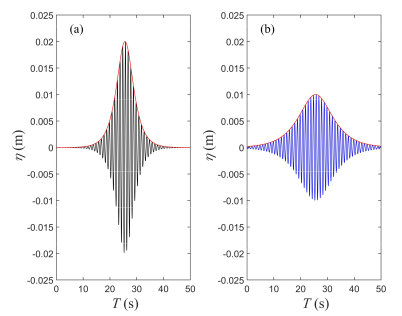
2. Brief Introduction of Solitons

The nonlinear Schrödinger equation describes the evolution of weakly nonlinear narrow-band wave trains. In deep water conditions, it was first derived by Zakharov [6]:
i A t + ω 0 2 k 0 A x ω 0 8 k 0 2 2 A x 2 ω 0 k 0 2 2 A 2 A = 0
where A(x, t) denotes the complex wave envelopes; x and t are spatial and time coordinates. The surface displacement η(x, t) is represented as:
η = Re A exp i ω 0 t k 0 x
where ω0 and k0 are the cyclic frequency and wavenumber of the carrier wave, and they are related according to the linear dispersion relation. As the NLS equation is always focusing in the deep water (it becomes de-focusing when k0h < 1.363), it admits a localized bright soliton solution given in the form [9]:
A x , t = A s o l sech 2 k 0 2 A s o l x c g t exp i k 0 2 ω 0 A s o l 2 t 4
where Asol is the maximum of the envelope soliton and cg = ω0 /2k0, cg is the linear group velocity corresponding to the carrier wave frequency. In the NLS framework, the envelope solitons are stable when propagating and interacting with other waves, including other solitons. A soliton has a sech-shaped profile and the theoretical surface displacement of envelope soliton can be derived from Equations (2) and (3):
η x , t = A s o l sech 2 k 0 2 A s o l x c g t cos ω 0 t 1 + k 0 2 A s o l 2 4 k 0 x
This equation indicates that the envelope of the soliton propagates at a speed of linear group velocity; however, the phase velocity of individual waves within the soliton takes into account the third-order nonlinear effects. Figure 1 shows two examples of the theoretical solitons with different amplitudes. It can be seen that the length of a soliton is inversely proportional to its height. The full width at half maximum of a soliton can be written as:
L s o l = 2 A s o l k 0 2 arcsech 1 2
and the corresponding duration is Tsol = Lsol/cg.

3. High-Order Spectral Model

The numerical simulations were performed using the HOS method which was first put forward by Dommermuth and Yue [31] and West et al. [28]. This method has been found to be an accurate and efficient numerical tool for direct phase-resolved simulation of nonlinear wave evolution [29,32]. The HOS method retains the full nonlinearity in the free surface conditions. In addition, this method has the ability to account for nonlinear interactions up to an arbitrary order M in steepness, using a number of free wave modes N to represent the sea-state. As in Zakharov [6], the potential on the free surface Φ(x, t) ≡ φ(x, η(x, t), t) is introduced to the free surface boundary conditions:
η t = ( 1 + η x η x ) v Φ x η x
Φ t = 1 2 ( 1 + η x η x ) v 2 η 1 2 Φ x Φ x
where v denotes the vertical velocity evaluated at the free surface. The main problem is to express v as a function of potential φ(x, z, t). To achieve this, the first step is to calculate the potential from the boundary–value problem through the pseudo-spectral method. The next step is to expand v in a Taylor series about the mean free surface z = 0:
v x , t = m = 1 M v m x , t = m = 1 M k = 0 m 1 η k k ! k + 1 z k + 1 φ m k x , z , t z = 0
v(m) and φ(m) indicate the quantity to be mth order in steepness and M is the desired order of nonlinearity. Substituting Equation (8) into Equations (6) and (7), the evolution equation for η and Φ is obtained. Given the initial values of η and Φ, unknowns of the next time step (η and Φ) can be obtained from the fourth order Runge–Kutta integration in time. In order to generate waves in the numerical wave tank, the wave maker condition is expanded to the second order. An additional potential that accounts for the wave maker is introduced and solved by the spectral method [33,34]. An absorbing layer is implemented on the opposite side of the wave maker to minimize the wave reflections. To achieve this, a term acting as a modification of the pressure [34] is added to Equation (7).

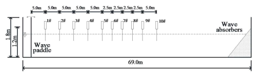
4. Numerical Flume Set-Up and Validation

The validation of the model was made by a comparison with the experimental results [35]. The experiments were conducted in a wave flume located at the State Key Laboratory of Coastal and Offshore Engineering, Dalian University of Technology, Dalian, China. The validation was intended to show the accuracy of the model to reproduce the evolution of long-crested irregular waves. The wave flume is 69.0 m long and 2.0 m wide with a water depth of 1.2 m. The experimental setup is shown in Figure 2. The flume was equipped with a piston-type wave maker and the origin of the horizontal coordinate was located at the mean position of the wave maker. A wave absorber was installed on the opposite side to minimize wave reflections. The random wave field was characterized by the Joint North SeaWave Project (JONSWAP) spectrum with different combinations of the bandwidth and steepness. The parameters of the wave conditions are specified in Table 1. The time series of the surface elevation measured at the first probe was decomposed into a number of independent harmonics and used to generate the input boundary conditions for numerical simulations. The experiments were reproduced with the following numerical settings: total duration T = 300 s and number of discretization nodes N = 2048. Although M = 3 is accurate enough for most cases [30], in order to guarantee almost fully nonlinear interactions, realizations were simulated with M = 6 in the present study.
Figure 3 shows the comparisons of the surface elevations between the numerical and experimental results at specified locations. The numerical simulations agreed well with the experiment. The wave amplitude and phase were correctly predicted by the HOS method. As fluid was assumed to be irrotational, inviscous, and bottom friction were neglected, the experiment was not perfectly reproduced. Minor differences were observed but they were acceptable. The successful comparisons with the experiments further validate the ability of the HOS method to simulate the evolution of long-crested random waves.

5. Results and Discussion

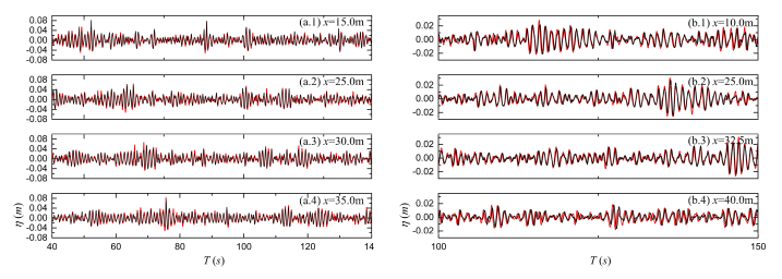
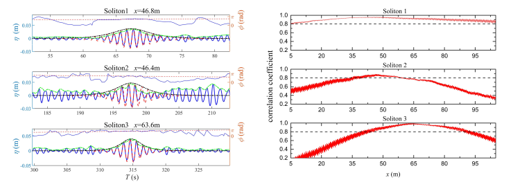
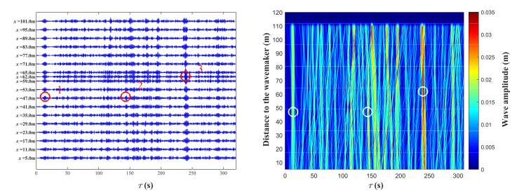
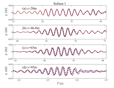
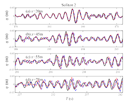
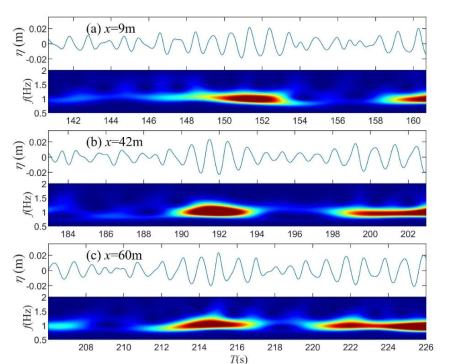
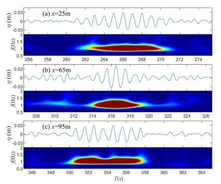
5.1. Identification of Solitons

After the accuracy of the HOS method was confirmed, we performed simulations with various initial conditions. Simulations of the wave group evolution were conducted in a numerical wave tank of 120 m long discretized with 2048 points. Each realization was simulated for 330 s with a time step of 0.02 s. The spatial domain contained about 100 individual waves and the duration of each simulation was about 330 wave periods. From the numerical results, we identified three typical solitons that emerged from the irregular wave trains.
A unidirectional random wave train was generated using the parameters of Case B. Figure 4 shows the evolution of the water surface elevations and the wave amplitude along the propagation direction; τ = t-x/cg was the coordinate in the frame that moved with the linear group velocity, and the group velocity corresponded to waves with a frequency equal to 1 Hz. There were many wave groups that emerged from this wave train. By visual inspection, three of the wave groups resembled soliton solutions, and required further analysis. These three solitons were labelled from 1 to 3 from left to right. It was noted that the length of these three wave groups was shortened during the formation of solitons, indicating a wave energy focusing process and resulting in high amplitude events. Then these wave groups developed into independent solitons and retained their shapes in a long-distance during propagation, while other groups dispersed due to the unbalance of the dispersion and the nonlinearity effects. Soliton 3 had a larger amplitude and it seems that this soliton existed from the beginning. Soliton 1 and Soliton 3 persisted for a relatively longer distance compared to Soliton 2. It was found that the group velocity of solitons nearly coincided with the linear group velocity, consistent with the expectation of the analytical solution.
Once the height and phase of a soliton is fixed, the theoretical envelope soliton profile can be determined. Therefore, a Hilbert transform was applied to obtain the local maxima of the envelope. The comparisons of the surface elevations and the corresponding instantaneous phases between the solitons emerged from the irregular waves and the theoretical envelope soliton profiles are presented in Figure 5 (left). The fit was considered to be successful when the correlation of the surface elevations was better than 80% [27]. The correlation coefficient is defined as the ratio between the covariance of the two compared soliton’s profile and the product of their standard deviations. We found that these three solitons agreed well with the theoretical soliton solution (Equation (4)) both for the surface elevations and the instantaneous phases [36]. The maximum wave heights of these three solitons remained nearly unchanged. We can also see, from the comparison of surface elevations, that the wave phase was in good agreement with the theoretical soliton solution for a long spatial evolution. The theoretical envelope soliton travelled at a speed of linear group velocity which again verifies that the simulated solitons propagated with the linear group velocity as well. The detected soliton’s envelope also matched the envelope of the theoretical soliton (Equation (3)). We noticed that, compared to the theoretical solitons, the detected soliton’s envelope was horizontal asymmetry. The asymmetry can be explained by the nonlinear effects which are not considered in the cubic NLS equation. Dysthe equations [37] with higher-order terms can account for the asymmetry features. This type of asymmetry was also observed in Feir’s experiments [38] and was confirmed by numerical simulations using the Dysthe equations [39]. Another striking phenomenon was that the emergence of Soliton 3 clearly resulted from a self-focusing process described in [40] and the envelope profile also resembled the Peregrine breather. However, the instantaneous phase heavily deviated from the theoretical Peregrine breather solution, and the remarkable feature of the Peregrine breather, the π jump, was not presented in Soliton 3. In addition, this soliton had a large amplitude from the beginning to the end, which also contradicts with the Peregrine breather whose energy is localized both in time and space. Compared to the experiments performed by Michel et al. [40], the steepness was smaller in this case, which indicates a weaker self-focusing process. Therefore, it was more similar to a soliton instead of a Peregrine breather.
These three typical solitons had different heights, and one soliton was identified as a freak wave. A freak wave is defined as a wave whose crest-to-trough excursion is twice as high as the significant wave height. The maximum wave height of Soliton 3 reached about 0.075 m and the amplification factor Hmax/Hs = 2.5 satisfied the rogue wave definition. It was also found that the taller the soliton was, the narrower its width was, consistent with Equation (5). All these three solitons had an amplitude larger than 1.4 times the significant wave height, which indicates that the formation of solitons is highly affected by wave amplitudes.

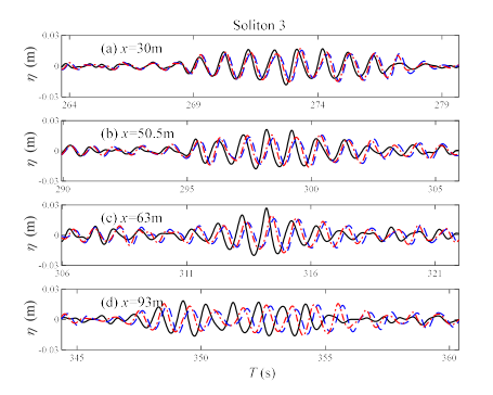
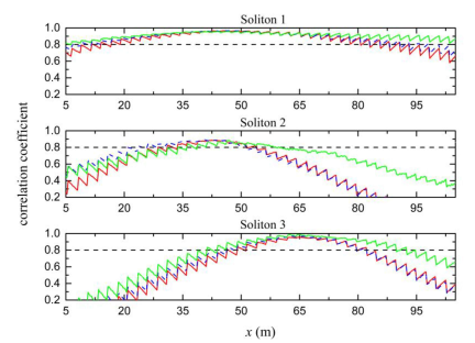
5.2. Persistence Distance of Solitons

The correlation coefficient between the simulated solitons and the theoretical solitons along the flume is presented in Figure 5 (right). The black dashed lines indicate the 80% threshold. The persistence distance of the soliton is the interval above the black dashed lines, and it can be clearly identified from Figure 5 (right). There are remarkable differences between the three solitons in terms of persistence distance.
For Soliton 1, the wave group already exhibited a soliton shape from the wave maker side and remained a qualified soliton till the end of the numerical tank. The correlation coefficient grew and reached its maximum of about 0.96 at x = 46.8 m, and then decreased; the persistence distance was the whole length of the wave tank which contained about 65 times the peak wavelength. For Soliton 2, it was hard to predict whether this wave group could evolve to a soliton in prior, since at the beginning there were no similarities between the shape of this wave group and a soliton. The wave group evolved progressively to a soliton at about x = 39.0 m, and the correlation coefficient attained its maximum at about x = 46.4 m. This soliton persisted for a relative short distance (20 m) which contained about 13 times the peak wavelength. For Soliton 3, the correlation coefficient increased to a maximum, reaching as high as 0.99 at x = 63.6 m and the persistence distance was about 32 times the peak wavelength (50 m).
In this sense, these three solitons were different considering the formation and persistence distance. Next, the formation details will be explained, respectively, for the three solitons.

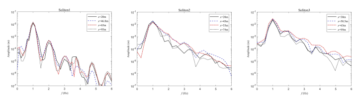
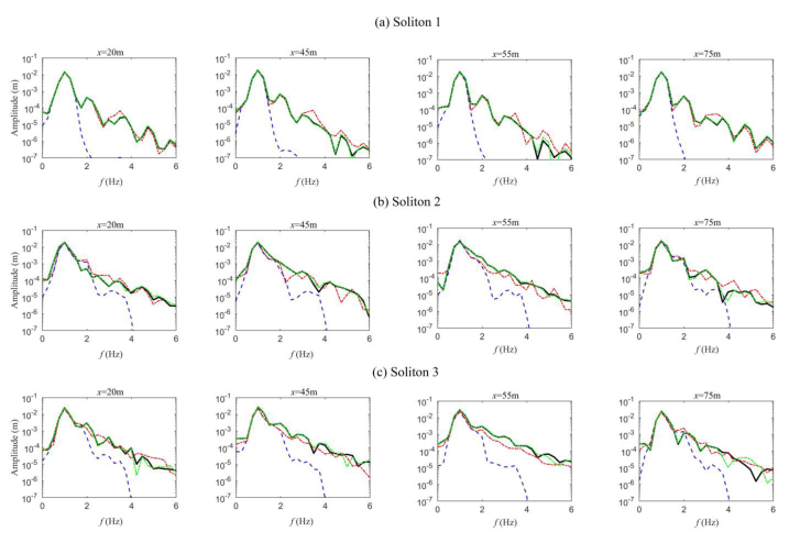
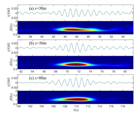
5.3. Formation of Solitons

To fully understand the formation process of solitons, the local wave groups at each location were extracted. Each wave group was centered at the maximum height of the soliton, and the time interval of the wave group was two times Tsol. The wave amplitude spectra obtained by Fourier transform at different locations along the flume are presented in Figure 6 for the three solitons. It is noted that for Soliton 1, the width of the spectrum slightly decreased during the evolutionary process. However, for Soliton 2, the wave spectrum underwent a significant change. The components at the higher sides of the peak frequency gained energy, and the width of the spectrum was broadened at x = 45 m and 55 m where the solitons emerged. When the solitons disappeared, the energy of the higher components decreased, and the width of the spectrum narrowed. The spectrum had a tendency of recurring back to the original state and the energy transfer seemed to be reversible. For Soliton 3, as seen in Figure 6 (right), the results were similar: the spectrum was also widened due to the emergence of solitons; as the soliton disappeared, the spectrum returned to a narrow one.
Simulations with only the linear effects (M = 1), second-order effects (M = 2), and third-order effects (M = 3) were also carried out in order to clarify what leads to the solitons and variations in the amplitude spectrum. Figure 7, Figure 8 and Figure 9 present the comparison of solitons observed in simulations with different nonlinearity parameters. As the surface elevations for M = 3 and M = 6 were almost identical, the time series for M = 3 is not pictured in these figures. It was noticed that in simulations with M = 1 and M = 2, solitons were still observed at the same location as M = 6. However, the solitons’ heights were lower than the previously observed solitons for M = 6. The persistence distance for M = 1 and M = 2 can be identified from the correlation coefficient curve in Figure 10. Due to the lack of nonlinearity, the balance between nonlinearity and dispersion was broken and the soliton’s shape could not hold as long as M = 6, so the persistence distance was shortened as well. The height and persistence distance for solitons of different nonlinear orders are listed in Table 2 and these indicate that nonlinearity has a positive effect on the stability of solitons. However, the height and persistence distance of the solitons were the same for M = 3 and M = 6, which means that nonlinear interactions higher than third order had no impact on the formation and stability of solitons. It is also noted that Soliton 1 had a longer persistence distance than the other two solitons. This was mainly because Soliton 1 had fewer surrounding waves and nearly no interactions with other waves.
It can be noted from Figure 11 that there were no remarkable changes in the amplitude spectrum for M = 1 and M = 2 during propagation, and again the spectrum was almost the same for M = 3 and M = 6, indicating that the third-order resonant interactions played a significant role in the formation of solitons [41,42]. Similar results have been observed in the study of freak waves and Peregrine breathers [43,44]. The above demonstrates the nonlinear wave energy transfer, especially the third-order resonant interactions were the main reason for the formation of solitons.
The spectral analysis only presented the energy variations within the wave group. To clearly demonstrate the interactions between solitons and surrounding waves, the time frequency analysis was also required. The wave energy distribution in the time and frequency domain was obtained through wavelet transform. The Morlet wavelet [45] was adopted in this study as the mother wavelet. The wavelet spectra at different locations are presented in Figure 12, Figure 13 and Figure 14. It is shown that the solitons gradually emerged from intense wave groups in the wave trains. For Soliton 2, it was found that before the emergence of solitons (x = 9 m, t (145 s, 155 s)), the spectra showed a down-chirp shape indicating that leading waves in the group had a higher frequency than the railing waves. When the solitons emerged, the length of the wave group decreased and wave energy gathered. The spectrum width also widened which is in accordance with previous results. At x = 60 m, when the solitons disappeared, the spectrum showed an up-chirp shape and the wave group dispersed. This process resembles a defocusing process. The analysis for Soliton 3 and Soliton 1 presented similar results. The above analysis shows the significance of linear dispersion to the formation of solitons.

6. Conclusions

The envelope soliton is an exact solution of the nonlinear Schrödinger (NLS) equation. It has a permanent and stable shape when propagating or interacting with other waves. Solitons and breathers are believed to be prototypes of rogue waves. In the present study, numerical simulations were performed to study soliton’s formation and evolution in a wave tank with the HOS method. The model was first validated by comparisons with experiments. In the numerical simulations, three solitons were identified during the evolution of irregular waves. The maximum height of a soliton can reach as high as Hmax/Hs = 2.5 satisfying the rogue wave definition. Solitons that emerged from irregular waves fitted the theoretical solution both in amplitude and instantaneous phases. It is verified that solitons travel at a speed of linear group velocity. Solitons in irregular waves exhibit horizontal asymmetry. Solitons can persist for a long distance with the envelope shape nearly unchanged. Wave groups that solitons located in were also analyzed by Fourier transform. The spectra bandwidth broadened during the formation of solitons; however, the spectra recurred back to a narrower one when the soliton disappeared. The Morlet wavelet transform was performed to characterize the energy distribution in the time–frequency domain. The wavelet spectra revealed that the peak frequency gradually decreased from the front to the rear before the soliton emerged; with further evolution, wave components were focused and energy gathered. When the solitons disappeared, the instantaneous frequencies in front became lower than those behind it, indicating a defocusing process. This whole process demonstrates that dispersive focusing also contributes to the formation of solitons.

Author Contributions

Methodology, Y.M., G.D. and X.M.; Data curation, Y.M.; software, W.X. and Y.M.; validation, X.M. and J.Z.; formal analysis, W.X., Y.M. and G.D.; investigation, Y.M. and X.M.; writing—original draft preparation, W.X. and Y.M.; writing—review and editing, W.X., Y.M. and J.Z.; supervision, Y.M. All authors have read and agreed to the published version of the manuscript.

Funding

This research was funded by the National Natural Science Foundation of China (Grant No. 51720105010, 51979029), LiaoNing Revitalization Talents Program (Grant No. XLYC1807010), and the Fundamental Research Funds for the Central Universities (Grant No. DUT2019TB02).

Institutional Review Board Statement

Not applicable.

Informed Consent Statement

Not applicable.

Data Availability Statement

Not applicable.

Conflicts of Interest

The authors declare no conflict of interest.

References

  1. Dysthe, K.; Krogstad, H.E.; Müller, P. Oceanic Rogue Waves. Annu. Rev. Fluid Mech. 2008, 40, 287–310. [Google Scholar] [CrossRef]
  2. Nikolkina, I.; Didenkulova, I. Rogue waves in 2006–2010. Nat. Hazards Earth Syst. Sci. 2011, 11, 2913–2924. [Google Scholar] [CrossRef]
  3. Kharif, C.; Pelinovsky, E. Physical mechanisms of the rogue wave phenomenon. Eur. J. Mech. B/Fluids 2003, 22, 603–634. [Google Scholar] [CrossRef] [Green Version]
  4. Lighthill, M.J. Contributions to the Theory of Waves in Non-linear Dispersive Systems. IMA J. Appl. Math. 1965, 1, 269–306. [Google Scholar] [CrossRef]
  5. Benjamin, T.B.; Feir, J.E. The disintegration of wave trains on deep water Part 1. Theory. J. Fluid Mech. 1967, 27, 417–430. [Google Scholar] [CrossRef]
  6. Zakharov, V. Stability of periodic waves of finite amplitude on the surface of a deep fluid. J. Appl. Mech. Tech. Phys. 1968, 9, 190–194. [Google Scholar] [CrossRef]
  7. Benney, D.J.; Newell, A.C. The Propagation of Nonlinear Wave Envelopes. J. Math. Phys. 1967, 46, 133–139. [Google Scholar] [CrossRef]
  8. Chu, V.H.; Mei, C.C. On slowly-varying Stokes waves. J. Fluid Mech. 1970, 41, 873–887. [Google Scholar] [CrossRef] [Green Version]
  9. Zakharov, V.E.; Shabat, A.B. Exact Theory of Two-dimensional Self-focusing and One-dimensional Self-modulation of Waves in Nonlinear Media. Sov. J. Exp. Theor. Phys. 1972, 34, 62. [Google Scholar]
  10. Chabchoub, A.; Onorato, M.; Akhmediev, N. Hydrodynamic Envelope Solitons and Breathers. In Rogue and Shock Waves in Nonlinear Dispersive Media; Onorato, M., Resitori, S., Baronio, F., Eds.; Springer International Publishing: Cham, Switzerland, 2016; pp. 55–87. ISBN 978-3-319-39214-1. [Google Scholar]
  11. Slunyaev, A.V. Analysis of the Nonlinear Spectrum of Intense Sea Wave with the Purpose of Extreme Wave Prediction. Radiophys. Quantum Electron. 2018, 61, 1–21. [Google Scholar] [CrossRef]
  12. Akhmediev, N.N.; Korneev, V.I. Modulation instability and periodic solutions of the nonlinear Schrödinger equation. Theor. Math. Phys. 1986, 69, 1089–1093. [Google Scholar] [CrossRef]
  13. Akhmediev, N.; Ankiewicz, A.; Taki, M. Waves that appear from nowhere and disappear without a trace. Phys. Lett. A 2009, 373, 675–678. [Google Scholar] [CrossRef]
  14. Dudley, J.M.; Genty, G.; Mussot, A.; Chabchoub, A.; Dias, F. Rogue waves and analogies in optics and oceanography. Nat. Rev. Phys. 2019, 1, 675–689. [Google Scholar] [CrossRef]
  15. Turitsyn, S.K.; Chekhovskoy, I.S.; Fedoruk, M.P. Nonlinear Fourier transform for characterization of the coherent structures in optical microresonators. Opt. Lett. 2020, 45, 3059–3062. [Google Scholar] [CrossRef]
  16. Chekhovskoy, I.S.; Shtyrina, O.V.; Fedoruk, M.P.; Medvedev, S.B.; Turitsyn, S.K. Nonlinear Fourier Transform for Analysis of Coherent Structures in Dissipative Systems. Phys. Rev. Lett. 2019, 122, 153901. [Google Scholar] [CrossRef] [PubMed] [Green Version]
  17. Suret, P.; Tikan, A.; Bonnefoy, F.; Copie, F.; Ducrozet, G.; Gelash, A.; Prabhudesai, G.; Michel, G.; Cazaubiel, A.; Falcon, E.; et al. Nonlinear Spectral Synthesis of Soliton Gas in Deep-Water Surface Gravity Waves. Phys. Rev. Lett. 2020, 125, 264101. [Google Scholar] [CrossRef]
  18. Sun, Y.-H. Soliton synchronization in the focusing nonlinear Schrödinger equation. Phys. Rev. E 2016, 93, 052222. [Google Scholar] [CrossRef]
  19. Bonnefoy, F.; Tikan, A.; Copie, F.; Suret, P.; Ducrozet, G.; Prabhudesai, G.; Michel, G.; Cazaubiel, A.; Falcon, E.; El, G.; et al. From modulational instability to focusing dam breaks in water waves. Phys. Rev. Fluids 2020, 5, 034802. [Google Scholar] [CrossRef] [Green Version]
  20. Clamond, D.; Grue, J. Interaction between envelope solitons as a model for freak wave formations. Part I: Long time interaction. Comptes Rendus Mécanique 2002, 330, 575–580. [Google Scholar] [CrossRef]
  21. Dyachenko, A.I.; Zakharov, V.E. On the formation of freak waves on the surface of deep water. JETP Lett. 2008, 88, 307–311. [Google Scholar] [CrossRef]
  22. Slunyaev, A.V. Numerical simulation of “limiting” envelope solitons of gravity waves on deep water. J. Exp. Theor. Phys. 2009, 109, 676–686. [Google Scholar] [CrossRef]
  23. Slunyaev, A.; Clauss, G.F.; Klein, M.; Onorato, M. Simulations and experiments of short intense envelope solitons of surface water waves. Phys. Fluids 2013, 25, 067105. [Google Scholar] [CrossRef] [Green Version]
  24. Slunyaev, A.; Klein, M.; Clauss, G.F. Laboratory and numerical study of intense envelope solitons of water waves: Generation, reflection from a wall, and collisions. Phys. Fluids 2017, 29, 47103. [Google Scholar] [CrossRef] [Green Version]
  25. Ducrozet, G.; Slunyaev, A.V.; Stepanyants, Y.A. Transformation of envelope solitons on a bottom step. Phys. Fluids 2021, 33, 066606. [Google Scholar] [CrossRef]
  26. Viotti, C.; Dutykh, D.; Dudley, J.; Dias, F. Emergence of coherent wave groups in deep-water random sea. Phys. Rev. E 2013, 87, 063001. [Google Scholar] [CrossRef] [Green Version]
  27. Cazaubiel, A.; Michel, G.; Lepot, S.; Semin, B.; Aumaître, S.; Berhanu, M.; Bonnefoy, F.; Falcon, E. Coexistence of solitons and extreme events in deep water surface waves. Phys. Rev. Fluids 2018, 3, 114802. [Google Scholar] [CrossRef] [Green Version]
  28. West, B.J.; Brueckner, K.A.; Janda, R.S.; Milder, D.M.; Milton, R.L. A new numerical method for surface hydrodynamics. J. Geophys. Res. Ocean. 1987, 92, 11803–11824. [Google Scholar] [CrossRef]
  29. Ducrozet, G.; Bonnefoy, F.; Le Touzé, D.; Ferrant, P. A modified High-Order Spectral method for wavemaker modeling in a numerical wave tank. Eur. J. Mech. B/Fluids 2012, 34, 19–34. [Google Scholar] [CrossRef]
  30. Ducrozet, G.; Bonnefoy, F.; Le Touzé, D.; Ferrant, P. HOS-ocean: Open-source solver for nonlinear waves in open ocean based on High-Order Spectral method. Comput. Phys. Commun. 2016, 203, 245–254. [Google Scholar] [CrossRef] [Green Version]
  31. Dommermuth, D.G.; Yue, D.K.P. A high-order spectral method for the study of nonlinear gravity waves. J. Fluid Mech. 1987, 184, 267–288. [Google Scholar] [CrossRef]
  32. Gouin, M.; Ducrozet, G.; Ferrant, P. Development and validation of a non-linear spectral model for water waves over variable depth. Eur. J. Mech. B/Fluids 2016, 57, 115–128. [Google Scholar] [CrossRef] [Green Version]
  33. Bonnefoy, F.; Le Touzé, D.; Ferrant, P. Generation of fully-nonlinear prescribed wave fields using a high-order spectral model. In Proceedings of the International Offshore and Polar Engineering Conference, Toulon, France, 23–28 May 2004; Volume 1, pp. 257–263. [Google Scholar]
  34. Bonnefoy, F.; Le Touzé, D.; Ferrant, P. A fully-spectral 3D time-domain model for second-order simulation of wavetank experiments. Part A: Formulation, implementation and numerical properties. Appl. Ocean Res. 2006, 28, 33–43. [Google Scholar] [CrossRef]
  35. Li, J.-X.; Li, P.-F.; Liu, S.-X. Observations of freak waves in random wave field in 2D experimental wave flume. China Ocean Eng. 2013, 27, 659–670. [Google Scholar] [CrossRef]
  36. Huang, N.E.; Long, S.R.; Tung, C.-C.; Donelan, M.A.; Yuan, Y.; Lai, R.J. The local properties of ocean surface waves by the phase-Time method. Geophys. Res. Lett. 1992, 19, 685–688. [Google Scholar] [CrossRef]
  37. Dysthe, K.B. Note on a modification to the nonlinear Schrödinger equation for application to deep water waves. Proc. R. Soc. Lond. Ser. A Math. Phys. Sci. 1979, 369, 105–114. [Google Scholar] [CrossRef]
  38. Feir, J.E. Discussion: Some results from wave pulse experiments. Proc. R. Soc. Lond. Ser. A Math. Phys. Sci. 1967, 299, 54–58. [Google Scholar] [CrossRef]
  39. Lo, E.; Mei, C.C. A numerical study of water-wave modulation based on a higher-order nonlinear Schrödinger equation. J. Fluid Mech. 1985, 150, 395–416. [Google Scholar] [CrossRef]
  40. Michel, G.; Bonnefoy, F.; Ducrozet, G.; Prabhudesai, G.; Cazaubiel, A.; Copie, F.; Tikan, A.; Suret, P.; Randoux, S.; Falcon, E. Emergence of Peregrine solitons in integrable turbulence of deep water gravity waves. Phys. Rev. Fluids 2020, 5, 082801. [Google Scholar] [CrossRef]
  41. Hasselmann, K. On the non-linear energy transfer in a gravity-wave spectrum Part 1. General theory. J. Fluid Mech. 1962, 12, 481–500. [Google Scholar] [CrossRef]
  42. Gibson, R.; Swan, C. The evolution of large ocean waves: The role of local and rapid spectral changes. Proc. R. Soc. A Math. Phys. Eng. Sci. 2007, 463, 21–48. [Google Scholar] [CrossRef]
  43. Ma, Y.; Dong, G.; Liu, S.; Zang, J.; Li, J.; Sun, Y. Laboratory Study of Unidirectional Focusing Waves in Intermediate Depth Water. J. Eng. Mech. 2010, 136, 78–90. [Google Scholar] [CrossRef]
  44. Dong, G.; Liao, B.; Ma, Y.; Perlin, M. Experimental investigation of the Peregrine Breather of gravity waves on finite water depth. Phys. Rev. Fluids 2018, 3, 064801. [Google Scholar] [CrossRef]
  45. Donelan, M.A.; Drennan, W.M.; Magnusson, A.K. Nonstationary Analysis of the Directional Properties of Propagating Waves. J. Phys. Oceanogr. 1996, 26, 1901–1914. [Google Scholar] [CrossRef] [Green Version]
Figure 1. Theoretical envelope soliton of Equation (4) with ω0 = 2π rad/s; (a) Asol = 0.02 m; (b) Asol = 0.01 m.
Jmse 09 01369 g001
Figure 2. Experimental setup.
Jmse 09 01369 g002
Figure 3. Comparisons of the surface elevations between the experimental data (black solid lines) and the numerical results (red solid lines) for Case A (left), and Case B (right).
Jmse 09 01369 g003
Figure 4. Left: Temporal evolution of the surface elevations at different locations (Case B: γ = 7.0, Hs = 0.03 m). Right: Spatiotemporal diagram of the wave envelope amplitude (Case B: γ = 7.0, Hs = 0.03 m).
Jmse 09 01369 g004
Figure 5. Left: Comparison between the detected soliton (blue solid line) and the theoretical envelope soliton profile (red dashed line). The black dashed line is the envelope of theoretical soliton. The green dashed line is the envelope of detected soliton. Right: Correlation coefficient between three wave groups and the theoretical solitons (red solid line) and the threshold to be successful solitons (black dashed line).
Jmse 09 01369 g005
Figure 6. The wave amplitude spectra at different locations along the flume for Soliton 1 (left), Soliton 2 (center), and Soliton 3 (right).
Jmse 09 01369 g006
Figure 7. Comparison of Soliton 1 between different nonlinear orders. The blue dashed lines correspond to the simulation with only linear effects (M = 1). The red dashed dot lines correspond to the simulation with second harmonic effects (M = 2). The black solid lines correspond to almost fully nonlinear simulations (M = 6).
Jmse 09 01369 g007
Figure 8. Comparison of Soliton 2 between different nonlinear orders. The blue dashed lines correspond to the simulation with only linear effects (M = 1). The red dashed dot lines correspond to the simulation with second harmonic effects (M = 2). The black solid lines correspond to almost fully nonlinear simulations (M = 6).
Jmse 09 01369 g008
Figure 9. Comparison of Soliton 3 between different nonlinear orders. The blue dashed lines correspond to the simulation with only linear effects (M = 1). The red dashed dot lines correspond to the simulation with second harmonic effects (M = 2). The black solid lines correspond to almost fully nonlinear simulations (M = 6).
Jmse 09 01369 g009
Figure 10. Correlation coefficient between three wave groups and theoretical solitons. The red solid lines correspond to the simulation with only linear effects (M = 1). The blue dashed lines correspond to the simulation with second harmonic effects (M = 2). The green solid lines correspond to the simulation with third-order nonlinear effects (M = 3). The black dashed lines correspond to the 80% threshold.
Jmse 09 01369 g010
Figure 11. The wave amplitude spectra at different locations along the flume for (a) Soliton 1, (b) Soliton 2, and (c) Soliton 3. The blue dashed lines correspond to the simulation with only linear effects (M = 1). The red dashed dot lines correspond to the simulation with second harmonic effects (M = 2). The green dashed dot lines correspond to the simulation with third-order nonlinear effects (M = 3). The black solid lines correspond to almost fully nonlinear simulations (M = 6).
Jmse 09 01369 g011
Figure 12. The time series and corresponding wavelet spectrum for Soliton 1 at three locations: (a) x = 30.0 m; (b) x = 50.0 m; (c) x = 80.0 m.
Jmse 09 01369 g012
Figure 13. The time series and corresponding wavelet spectrum for Soliton 2 at three locations: (a) x = 9.0 m; (b) x = 42.0 m; (c) x = 60.0 m.
Jmse 09 01369 g013
Figure 14. The time series and corresponding wavelet spectrum for Soliton 3 at three locations: (a) x = 25.0 m; (b) x = 65.0 m; (c) x = 95.0 m.
Jmse 09 01369 g014
Table 1. Wave parameters measured at the first location x = 5.0 m.
Hs (m)Tp (s)kphε = kpHs/2γΔf/fp
Case A0.0641.04.820.123.30.10
Case B0.031.04.820.067.00.07
Note: Hs: significant wave height; Tp: peak period; kp: wavenumber corresponding to the peak period; kph: relative water depth; ε: wave steepness; γ: peak enhancement factor of the spectrum; Δf: full width at half maximum of the spectrum; Δf/fp: relative bandwidth.
Table 2. The height and persistence distance of solitons for different nonlinear orders.
M = 1M = 2M = 3M = 6
Soliton 1Asol (m)0.01960.02070.02250.0225
L/Lp45.849.867.367.3
Soliton 2Asol (m)0.02680.02770.02850.0285
L/Lp13.214.515.615.6
Soliton 3Asol (m)0.02930.03340.04040.0404
L/Lp20.922.732.232.2
Note: Asol: soliton’s height; L: persistence distance of soliton; Lp: wavelength corresponding to the peak period.
Publisher’s Note: MDPI stays neutral with regard to jurisdictional claims in published maps and institutional affiliations.

