Article

Identification of Ship Hydrodynamic Derivatives Based on LS-SVM with Wavelet Threshold Denoising

1
Key Laboratory of High Performance Ship Technology, Wuhan University of Technology, Ministry of Education, Wuhan 430070, China
2
School of Naval Architecture, Ocean and Energy Power Engineering, Wuhan University of Technology, Wuhan 430070, China
*
Authors to whom correspondence should be addressed.
J. Mar. Sci. Eng. 2021, 9(12), 1356; https://doi.org/10.3390/jmse9121356
Submission received: 19 October 2021 / Revised: 16 November 2021 / Accepted: 23 November 2021 / Published: 1 December 2021
(This article belongs to the Special Issue Manoeuvring and Control of Ships and Other Marine Vehicles)

Abstract

:
Nowadays, system-based simulation is one of the main methods for ship manoeuvring prediction. Great efforts are usually devoted to the determination of hydrodynamic derivatives as required for the mathematical models used for such methods. System identification methods can be applied to determine hydrodynamic derivatives. The purpose of this work is to present a parameter identification study based on least-squares support-vector machines (LS-SVMs) to obtain hydrodynamic derivatives for an Abkowitz-type model. An approach for constructing training data is used to reduce parameter drift. In addition, wavelet threshold denoising is applied to filter out the noise from the sample data during data pre-processing. Most of the resulting derivatives are very close to the original ones—especially for linear derivatives. Although the errors of high-order derivatives seem large, the final predicted results of the turning circle and zigzag manoeuvres agree pretty well with the reference ones. This indicates that the used methods are effective in obtaining manoeuvring hydrodynamic derivatives.

1. Introduction

With the development of large-scale and professional ships over past decades, ships have become more difficult to control, and accidents may occur. Navigational safety issues related to manoeuvrability have attracted much attention worldwide recently. The International Maritime Organization (IMO) has formulated standards for ship manoeuvrability [1] to improve the quality of ship design and manufacturing. In addition, with the introduction of the concept of green ships, energy-saving and emission reduction have become vital goals. Accurate ship manoeuvring prediction can help control ships in an appropriate manner and reduce energy consumption.
There are usually two methods for evaluating ship manoeuvrability at the initial stage of design. One is to perform free-running tests, which can directly obtain the characteristic parameters including advance, transfer, tactical diameter, overshoot angles, etc. The other is to predict manoeuvring performances based on system simulations. For the latter, the Abkowitz-type model [2] is one of the most widely used ship manoeuvring mathematic models. However, many hydrodynamic derivatives need to be determined in advance. Therefore, it is essential to obtain hydrodynamic derivatives when an Abkowitz-type model is applied to predict ship manoeuvring motion.
Common methods for obtaining hydrodynamic derivatives may include databases, empirical formulae, captive model tests, computational fluid dynamics (CFD) calculations, and system identification (SI). The SI-based approach is an effective and convenient method that is less costly. Moreover, this method can be applied to full-scale trials to avoid scale effects. There have been many successful applications of SI methods for the determination of hydrodynamic derivatives over past decades. Traditional SI methods may include least-squares (LS) estimation [3], improved least-squares [4], extended Kalman filter (EKF) [5], and recursive prediction error (RPE) [6] methods. However, the application of these methods is limited due to some issues. For example, such methods are highly dependent on the selection of initial values and are sensitive to noise. With the development of artificial intelligence, some new SI methods are expected to overcome these defects, such as artificial neural networks (ANN) [7], support vector machines (SVMs), Bayesian optimisation (BO) [8], genetic algorithms and optimisation methods [9]. In this paper, SVM is used to identify hydrodynamic derivatives. SVMs have good generalisation performance and global optimal solutions. Furthermore, they can effectively avoid the problem of dimensionality, and there is no dependence on the initial parameter estimates. In recent years, Luo and Zou identified the hydrodynamic derivatives of the Abkowitz-type model by using a least-squares support-vector machine (LS-SVM) algorithm [10]. Then, particle swarm optimisation (PSO) [11] and the artificial bee colony algorithm (ABC) [12] were applied to find the optimal hyper-parameter in the LS-SVM algorithm. However, the LS-SVM algorithm still has a shortcoming, which is the lack of sparsity of the solution. To overcome this problem, ε - SVM was applied to adjust the sparsity of the solution and to identify the hydrodynamic derivatives [13]. Besides this, some black-box modelling methods that do not need hydrodynamic derivatives were also applied to predict ship manoeuvring motion [14,15,16].
In the application of an identification method, the accuracy of the identification results is closely related to the training data. However, the training data obtained from experiments often contain noise. Meanwhile, the structure of the high-fidelity manoeuvring model is usually very complex and redundant. Such models are often prone to over-fitting [17]. In previous studies, most scholars directly used noisy data when applying identification methods. For example, Sutulo and Guedes Soares developed a classic genetic algorithm using the Hausdorff metric, and it was validated using simulated responses polluted with white noise [9]. Xue and Liu et al. used Gaussian process regression to identify a dynamic model with input noise [18]. Wang and Zou et al. applied an improved nu-SVM to predict ship manoeuvring motion with input noise [19]. However, few scholars consider applying denoising methods to the processing of training data. Moreover, parameter identification results are usually far from the true values [20]. This phenomenon may be caused by parameter drift. Parameter drift is a common problem when the SI method is applied to obtain model parameters. To diminish parameter drift, some scholars have tried several methods. Hwang applied “parallel processing” to process the training data but did not completely eliminate parameter drift [20]. Shenoi et al. simplified Son and Nomoto’s nonlinear model using sensitivity analysis [21]. Yoon and Rhee reduced parameter drift by modifying the input scenario [22]. Luo and Li reduced the multicollinearity in the input matrix by adding excitation to the training samples [23]. Luo reduced multicollinearity using a difference method and an additional signal method [24]. Most of these methods are mainly from the perspective of reconstructing training samples to reduce parameter drift. Their results indicate that parameter drift cannot be eliminated, but can be significantly reduced.
Recently, wavelet threshold denoising [25] has drawn attention in marine engineering. Wavelet threshold denoising is a theory based on wavelet analysis. As a new time-frequency analysis method, wavelet analysis is known as the “mathematical microscope”, because of its ability to perform multi-resolution analysis, which can focus on any details in the signal for performance of multi-resolution time-frequency analysis. Therefore, wavelet threshold denoising has been widely applied to data pre-processing. Zhang and Zou applied wavelet threshold denoising to filter out the noise in the training data and then used the denoised training data to identify the response model [26]. However, the response model contains only a few parameters, and the prediction accuracy of the response model is not very high.
In this study, an LS-SVM method with wavelet threshold denoising is introduced into the identification process of hydrodynamic derivatives for an Abkowitz-type model. The hydrodynamic derivatives, based on Reynolds-averaged Navier–Stokes (RANS) simulations, are used to obtain the original training data. The wavelet threshold denoising is applied to filter out the noise from the polluted training data during data pre-processing. The hydrodynamic derivatives in the Abkowitz-type model are identified by LS-SVM. A modified regression model is used to reduce parameter drift without adding additional excitation, which usually has to be considered in traditional approaches. Generalisation performance of the identified model is evaluated by predicting manoeuvring motions not included in the training data.
The structure of the paper is organized as follows: Section 2 describes the ship mathematical model. The algorithms of LS-SVM are presented in Section 3. In Section 4, the regression model and the wavelet threshold denoising algorithm are described. Moreover, a simulated experimental example is presented to demonstrate the validity of the identified model. Section 5 summarizes the study with conclusions.

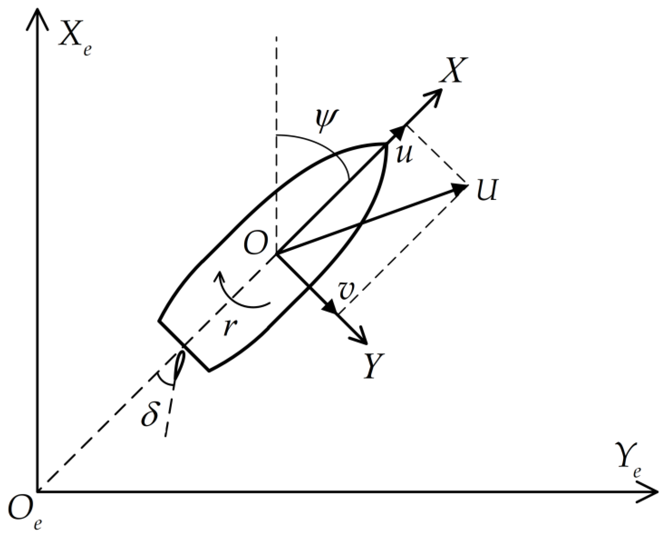
2. Mathematical Model of Ship Manoeuvring Motion

To describe ship motion, two coordinate reference systems were used here, as shown in Figure 1. One was the earth-fixed coordinates O e X e Y e Z e ; the other was the body-fixed coordinates O X Y Z , where u , v , r were the surge velocity, sway velocity and yaw rate, respectively, ψ was the heading angle, and δ was the rudder angle.
According to Newton’s law, the equations for surge motion, sway motion and yaw motion can be written as follows:
m ( u ˙ v r x G r 2 ) = F X m ( v ˙ + u r + x G r ˙ ) = F Y I Z r ˙ + m x G ( v ˙ + u r ) = F N
where m is ship mass; x G is the longitudinal coordinate of the ship gravity center in the body-fixed coordinate system; I Z is the moment of inertia about the Z axis; F X , F Y , F N are the longitudinal force, transverse force and yaw moment; according to the Abkowitz-type model [2], the hydrodynamic forces and moment on the right side of Equation (1) may be approximated by the following expressions:
F X = X u Δ u + X u u ( Δ u ) 2 + X v v v 2 + X u ˙ u ˙ + X r r r 2 + X v r v r + X δ δ δ 2 + X v δ v δ + X r δ r δ F Y = Y v v + Y v v v 2 + Y v v v v 3 + Y v ˙ v ˙ + Y r r + Y r r r 2 + Y r r r r 3 + Y r ˙ r ˙ + Y δ δ + Y δ δ δ 2 + Y δ δ δ δ 3 + Y v r r v r 2 + Y v v r v 2 r + Y u δ Δ u δ + Y v δ δ v δ 2 + Y v v δ v 2 δ + Y r δ δ r δ 2 + Y r r δ r 2 δ F N = N v v + N v v v 2 + N v v v v 3 + N v ˙ v ˙ + N r r + N r r r 2 + N r r r r 3 + N r ˙ r ˙ + N δ δ + N δ δ δ 2 + N δ δ δ δ 3 + N v r r v r 2 + N v v r v 2 r + N u δ Δ u δ + N v δ δ v δ 2 + N v v δ v 2 δ + N r δ δ r δ 2 + N r r δ r 2 δ
Equation (2) is substituted into Equation (1), and they are rewritten in a dimensionless form. The acceleration terms are then on the left side, and the other terms are on the right side. By doing this, the following equations are obtained:
( m X u ˙ ) u ˙ = F 1 ( u , v , r , δ ) ( m Y v ˙ ) v ˙ + ( m x G Y r ˙ ) r ˙ = F 2 ( u , v , r , δ ) ( m x G N v ˙ ) v ˙ + ( I Z N r ˙ ) r ˙ = F 3 ( u , v , r , δ )
F 1 = X u Δ u + X u u ( Δ u ) 2 + X v v v 2 + ( m x G + X r r ) r 2 + ( m + X v r ) v r + X δ δ δ 2 + X v δ v δ + X r δ r δ F 2 = m u r + Y v v + Y v v v 2 + Y v v v v 3 + Y r r + Y r r r 2 + Y r r r r 3 + Y δ δ + Y δ δ δ 2 + Y δ δ δ δ 3 + Y v r r v r 2 + Y v v r v 2 r + Y u δ ( Δ u ) δ + Y v δ δ v δ 2 + Y v v δ v 2 δ + Y r δ δ r δ 2 + Y r r δ r 2 δ F 3 = m x G u r + N v v + N v v v 2 + N v v v v 3 + N r r + N r r r 2 + N r r r r 3 + N δ δ + N δ δ δ 2 + N δ δ δ δ 3 + N v r r v r 2 + N v v r v 2 r + N u δ ( Δ u ) δ + N v δ δ v δ 2 + N v v δ v 2 δ + N r δ δ r δ 2 + N r r δ r 2 δ
where F 1 , F 2 , F 3 are the polynomials related to the state information, as shown in Equation (4), the change of surge speed relative to the initial surge velocity u 0 is Δ u = u u 0 .

3. Least-Squares Support-Vector Machine

Least-squares support-vector machine (LS-SVM) is an improved support-vector machine (SVM) based on statistical theory [27]. Traditional SVM needs to solve an inequality constraint, which increases the computing time. LS-SVM can transform the inequality constraints in traditional SVM to equality constraints, and uses the error squared loss function as the experience loss of the training set. This greatly simplifies the calculation process. Therefore, LS-SVM has been successfully applied to the field of system identification. Its specific algorithm is introduced in the following:
Suppose the training sample is given as T = { x i , y i } i = 1 k , where k is the number of training samples, x i R k is the input variable, and y i R k is the output variable. The nonlinear function Φ ( x ) = { φ ( x i ) } i = 1 n is selected to map the input space to the feature space. The form of the nonlinear function modeling is:
y ( x ) = w T φ ( x ) + b
where w is a weight matrix and b is the bias term. According to the risk minimization principle, the constraint problem can be established as:
{ min w , b , e J ( w , e ) = 1 2 w 2 + γ 2 i = 1 n e i 2 s . t . y i = w T φ ( x i ) + b + e i     i = 1 , 2 , , n
where w 2 is the regularized part; γ is the regularization parameter; e i is the error between the model and the training sample; and e is the error variable. By introducing the Lagrange multiplier α , Equation (6) can be written as:
L ( w , b , e i , α ) = 1 2 w 2 + γ 2 i = 1 n e i 2 i = 1 n [ α i ( w T φ ( x i ) + b y i ) ]
According to the Karush–Kuhn–Tucker conditions (KKT) [28], the following formula can be obtained:
{ L w = 0 w = i = 1 n α i φ ( x i ) L b = 0 i = 1 n α i = 0 L e i = 0 γ e i = α i    i = 1 , , n L α i = 0 y i = w T φ ( x i ) + b + e i    i = 1 , , n
The α i and b in Equation (8) can be obtained using the following solution:
[ 0 s T s K ( x i , x j ) + γ 1 I ] [ b α ] = [ 0 y ]
where α = [ α 1 , α 2 , α n ] T , y = [ y 1 , y 2 , y n ] T , s = [ 1 , 1 , , 1 ] T , I is the identity matrix, and K ( x i , x j ) is the kernel function:
K ( x i , x j ) = φ ( x i ) , φ ( x j )
where , is the inner product of the eigenspace. The common kernel functions are the linear kernel function, polynomial kernel function, RBF kernel function, and sigmoid kernel function. Referring to the work of Luo and Zou [10], the linear kernel function is adopted in this study. The linear kernel is defined as follows:
K ( x i , x j ) = x i T x j
The final function model can be obtained as:
f ( x ) = i = 1 n ( α i K ( x , x i ) ) + b

4. Case Study

4.1. Construction of Regression Model
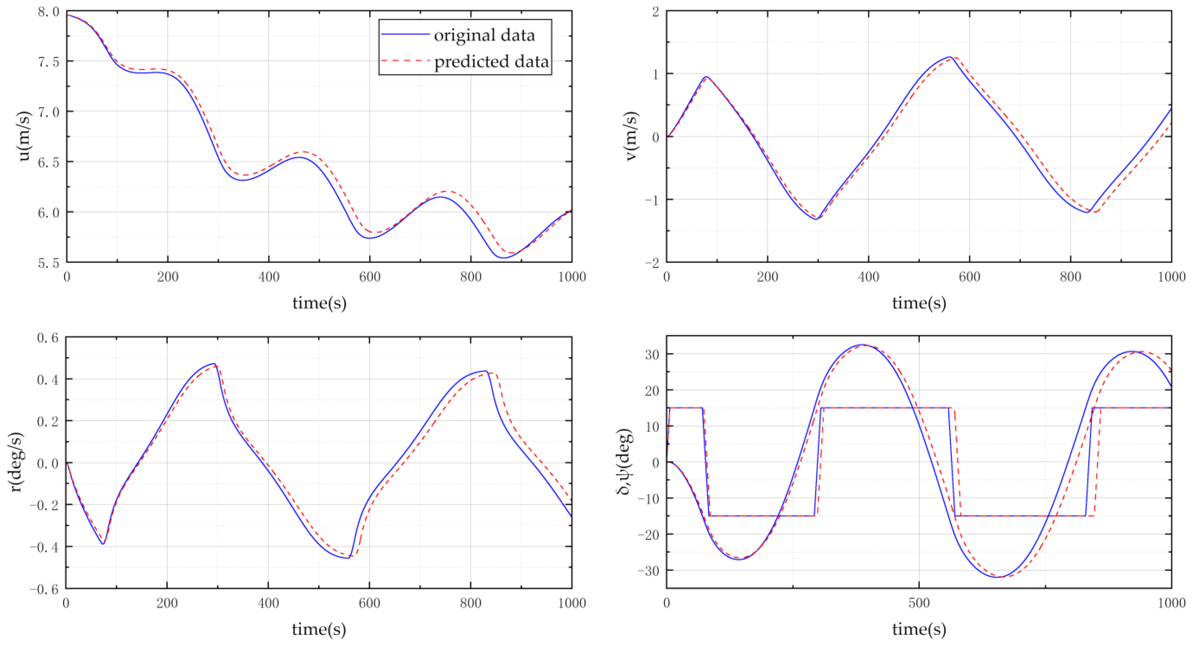
As mentioned above, parameter drift is a significant problem when the regression method is applied to obtain hydrodynamic derivatives. Parameter drift is caused by multicollinearity in the regression model. Multicollinearity means that although the results of the function fitting are perfect, the results of parameter identification will still show significant deviations. Luo and Li reduced multicollinearity by adding additional excitation to the training samples [23]. In this study, a modified regression model was used to identify hydrodynamic derivatives without adding additional excitation. The detailed structure of the regression model is described below.
Equation (4) can be rewritten as:
F 1 m x G r 2 m v r = X A ( i ) F 2 + m u r = Y B ( i ) F 3 + m x G u r = N C ( i )
where the hydrodynamic derivatives and speed state variables in Equation (13) are as follows:
X = [ X u , X u u , X v v , X r r , X v r , X δ δ , X v δ , X r δ ] 1 × 8 Y = [ Y v , Y v v , Y v v v , Y r , Y r r , Y r r r , Y δ , Y δ δ , Y δ δ δ , Y v r r , Y v v r , Y u δ , Y v δ δ , Y v v δ , Y r δ δ , Y r r δ ] 1 × 16 N = [ N v , N v v , N v v v , N r , N r r , N r r r , N δ , N δ δ , N δ δ δ , N v r r , N v v r , N u δ , N v δ δ , N v v δ , N r δ δ , N r r δ ] 1 × 16 A ( i ) = [ Δ u ( i ) , Δ u 2 ( i ) , v 2 ( i ) , r 2 ( i ) , v ( i ) r ( i ) , δ 2 ( i ) , v ( i ) δ ( i ) , r ( i ) δ ( i ) ] 1 × 8 T B ( i ) = [ v ( i ) , v 2 ( i ) , v 3 ( i ) , r ( i ) , r 2 ( i ) , r 3 ( i ) , δ ( i ) , δ 2 ( i ) , δ 3 ( i ) , v ( i ) r 2 ( i ) , v 2 ( i ) r ( i ) , Δ u ( i ) δ ( i ) , v ( i ) δ 2 ( i ) , v 2 ( i ) δ ( i ) , r ( i ) δ 2 ( i ) , r 2 ( i ) δ ( i ) ] 1 × 16 T C ( i ) = [ v ( i ) , v 2 ( i ) , v 3 ( i ) , r ( i ) , r 2 ( i ) , r 3 ( i ) , δ ( i ) , δ 2 ( i ) , δ 3 ( i ) , v ( i ) r 2 ( i ) , v 2 ( i ) r ( i ) , Δ u ( i ) δ ( i ) , v ( i ) δ 2 ( i ) , v 2 ( i ) δ ( i ) , r ( i ) δ 2 ( i ) , r 2 ( i ) δ ( i ) ] 1 × 16 T
where X , Y , N are the unknown terms containing the hydrodynamic derivatives. The structure of the regression model for identification can be written as follows:
Input variables: [ A ( i ) , B ( i ) , C ( i ) ]
Output response:
[ ( m X u ˙ ) L u ˙ u 2 ( i ) m x G L 2 r 2 ( i ) u 2 ( i ) m L v ( i ) r ( i ) u 2 ( i ) ( m Y v ˙ ) L v ˙ u 2 ( i ) + ( m x G Y r ˙ ) L 2 r ˙ u 2 ( i ) + m L u ( i ) r ( i ) u 2 ( i ) ( m x G N v ˙ ) L v ˙ u 2 ( i ) + ( I Z N r ˙ ) L 2 r ˙ u 2 ( i ) + m x G L u ( i ) r ( i ) u 2 ( i ) ]
u ˙ , v ˙ , r ˙ can be obtained by discretization using the explicit Euler scheme as follows:
u ˙ = u ( i + 1 ) u ( i ) Δ t , v ˙ = v ( i + 1 ) v ( i ) Δ t , r ˙ = r ( i + 1 ) r ( i ) Δ t
where Δ t is the time step and i and i + 1 are two consecutive time steps. Then, the input variables and output response were input into the LS-SVM to verify the validity of the modified regression model in the next section.

4.2. Identification

The second variant of Korea Very Large Crude Carrier (KVLCC2) was selected for the present case study. The main particulars of KVLCC2 are shown in Table 1.
In order to obtain the training data, the hydrodynamic derivatives based on RANS simulations were used to simulate ship free-running motions. To this end, a series of captive model tests for KVLCC2, such as static drift motion, static circle motion, dynamic sway motion, dynamic yaw motion, etc., were simulated by the RANS method to obtain the hydrodynamic forces. Hydrodynamic derivatives were then determined by regression analysis of the RANS results. More details on RANS computations can be found in the work of Yao et al. [29]. A 20 ° / 20 ° zigzag test was simulated by using the Abkowitz-type model, where the hydrodynamic derivatives were obtained by RANS computations. The sampling interval was 1 s, and the sampling time was 1000 s. The regularization parameter γ = 10 7 was chosen. The identification results of the LS-SVM are shown in Table 2. The acceleration derivatives, including X u ˙ , Y v ˙ , Y r ˙ , N v ˙ and N r ˙ , were calculated by RANS computations. The values of these derivatives were as follows: X u ˙ = 0.001135 , Y v ˙ = 0.014508 , Y r ˙ = 0.001209 , N v ˙ = 0.000588 , N r ˙ = 0.000564 .
The results in Table 2 show that most of the hydrodynamic derivatives were accurately determined. These results indicate that the regression model is valid. However, due to an error of the sensor and various external uncertain disturbances, including wind, waves, and current, the training samples obtained from the actual experiment were noisy compared with the simulated ones. Therefore, for real situations, the results obtained will have a significant deviation when the LS-SVM directly identifies hydrodynamic derivatives. For this, wavelet threshold denoising was employed here to reduce interference in the data. Based on Sutulo and Soares’s method of noise generation [9], Gaussian white noise was added to the sample data to simulate the real situation. The detailed process was as follows:
ζ i = ζ 0 i + ζ max k 0 k ζ ζ i
where ζ = u , v , r , δ , ζ 0 i is the original “clean” reference data, ζ max is the maximum absolute value of the clean data, k 0 is the general reduction factor used to represent different noise levels—which is set to 5 % in this study— k ζ is a specific reduction factor based on the values of different variables, and ζ i is a random variable with a variance of 0.2 following Gaussian distribution. According to the records of previous experimental data, the noise of the ship surge velocity is significantly less than the rate of yaw and drift angle, and the noise of the rudder angle can be ignored. Therefore, the reduction factor k ζ was set to 0.2 for the surge velocity and 1.0 for the remaining responses.

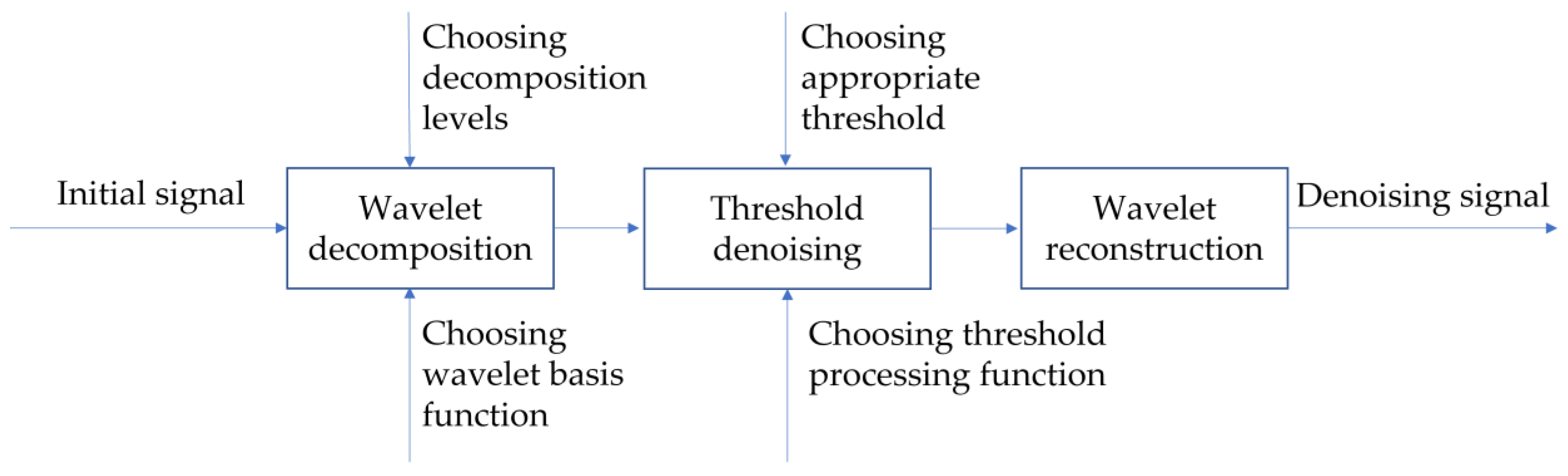
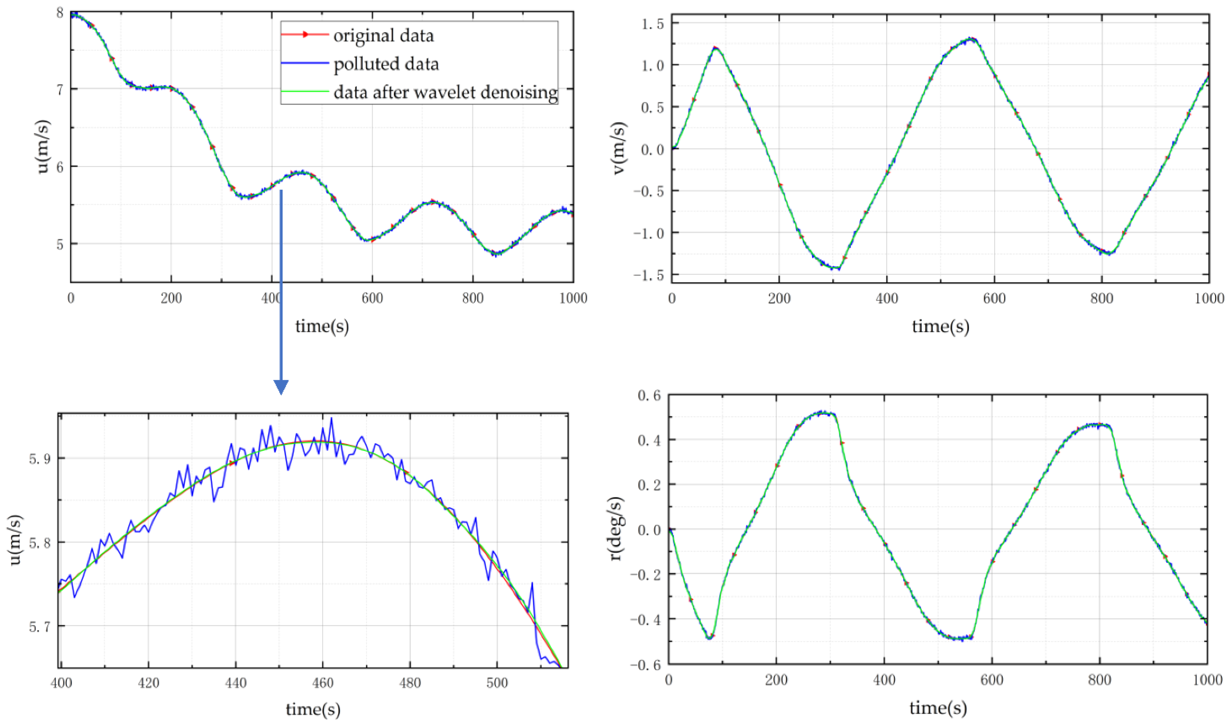
4.3. Wavelet Threshold Denoising

Commonly, a signal model with noise can be written as follows:
s ( t ) = f ( t ) + n ( t )
where s ( t ) is the signal with noise; f ( t ) is the original effective signal; and n ( t ) is the noise signal. The purpose of denoising is to reduce n ( t ) in s ( t ) .
The basic idea of wavelet threshold denoising [25] is to transform the signal and gene-rate wavelet coefficients. These wavelet coefficients contain vital signal information. In general, an effective signal is a low-frequency signal, and a noise signal is a high-frequency signal. The effective signal has a certain continuity in the time domain. However, the noise signal is discontinuous in the time domain. Therefore, the wavelet coefficients of effective signals are usually large, whereas the wavelet coefficients of noise signals are generally small. An appropriate threshold is required here. When the wavelet coefficient of the signal is greater than the threshold value, it is retained. When the wavelet coefficient of the signal is less than the threshold, it is set to zero. Figure 2 is the flow chart for wavelet threshold denoising.
The implementation steps of wavelet threshold denoising are as follows:
Step 1: Wavelet decomposition. Wavelet basis function and decomposition levels need to be determined in this step. Wavelet basis function is chosen by observing the initial sign s ( t ) . Daubechies 4 wavelet [26] was selected in this study. The decomposition level is a vital parameter in the filtering process. On one hand, noise separation is more effective when the decomposition level is larger. On the other hand, excessive decomposition levels can result in the loss of effective signal. The decomposition level is usually determined by pre-tests. In this study, the decomposition level was five after testing.
Step 2: Threshold processing. This step includes the selection of wavelet threshold and threshold processing functions. The heuristic threshold [30] is an ordinary wavelet threshold. The specific algorithm of the heuristic threshold is as follows:
f ( k ) = ( s o r t | s | ) 2     ( k = 1 , 2 , N ) r ( k ) = [ N 2 k + i = 1 k f ( i ) + ( N k ) f ( N k ) ] / N λ 1 = min ( r )     λ 2 = 2 ln ( N )
where s is the initial signal; N is the length of the signal; s o r t means ascending order; k is the moment; r ( k ) is the value of risk at that moment; and λ is the threshold value. The formula for the heuristic threshold can be written as:
e t a = [ k = 1 N | s k | 2 N ] / N     c r i t = 1 N ( ln N ln 2 ) 3 λ = { λ 2 e t a < c r i t min ( λ 1 , λ 2 ) e t a c r i t
The usual threshold processing functions are the hard threshold processing function and the soft threshold processing function [31]. In this study, the latter is adopted. The specific algorithm is as follows:
w = { [ sgn ( w ) ] ( | w | λ ) | w | λ 0 | w | < λ
where w is the original wavelet coefficient, w is the denoised wavelet coefficient.
Step 3. Wavelet reconstruction. According to the denoised wavelet coefficients obtained above, the inverse transform of wavelet decomposition is applied to reconstruct the denoising signal.
According to Equation (17), polluted 20 ° / 20 ° zigzag test data can be obtained. The above methods were applied to denoise the polluted data. The comparison of original data, polluted data and denoised data are shown in Figure 3. It can be seen from the enlarged surge velocity comparison graph that the wavelet threshold denoising had a good denoising performance. Following this, the denoised data was brought into the regression model for identification by the LS-SVM. The regularization parameter γ = 10 4 was chosen here. The results of identification are shown in Table 3.
It can be observed from Table 3 that most of the predicted hydrodynamic derivatives were relatively accurate. However, some high-order hydrodynamic derivatives had significant errors. One possible reason is the influence of the wavelet threshold denoising process. As mentioned in Section 4.3, the choice of wavelet decomposition levels and the wavelet threshold will affect the denoising process. Therefore, one possible explanation is that the noise in the data was not completely filtered out, or that the wavelet decomposition levels were too large to filter out part of the effective signal. Another possible reason is parameter drift. As mentioned in Section 4.1, the fundamental reason for parameter drift is multicollinearity in the regression model. Although the phenomenon of parameter drift is not obvious when using clean data for identification, the problem of multicollinearity still exists in the regression model. When polluted data is used for identification, the noise may aggravate the multicollinearity in the model and make the parameter drift more obvious. In addition, high-order hydrodynamic derivatives may be more sensitive. There may not be enough information to identify them in the training data. In general, although the predictions of some high-order hydrodynamic derivatives were not sufficiently accurate, it does not mean that the identified model cannot be used to predict the manoeuvring motion.

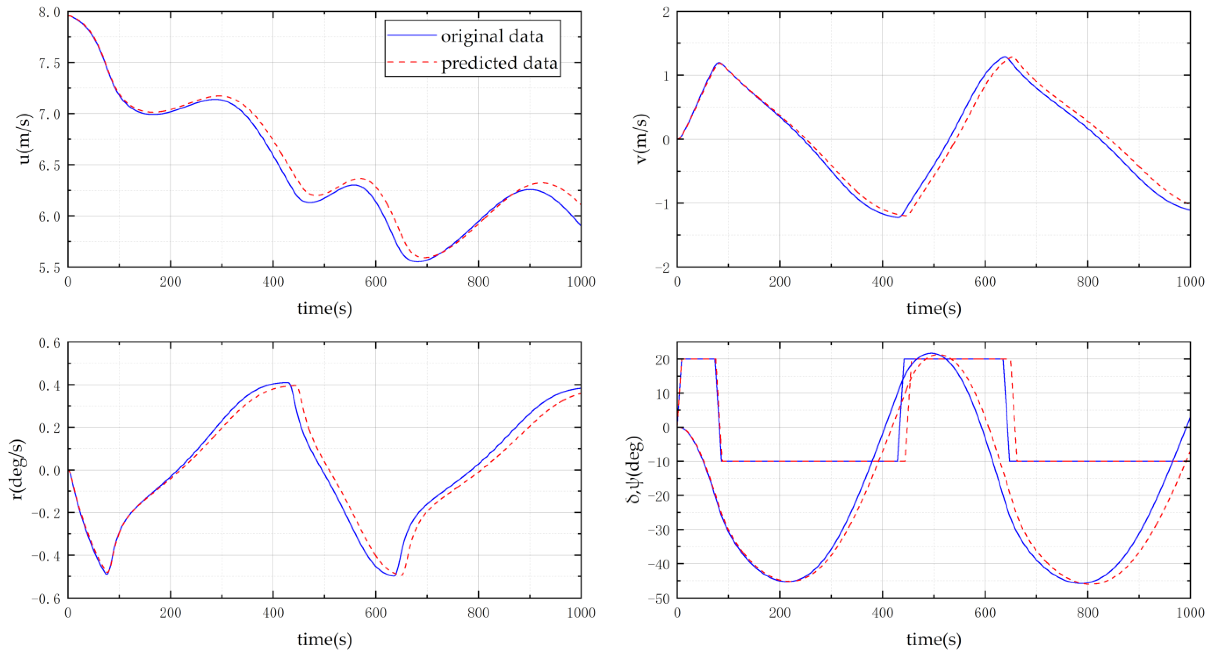
4.4. Model Validation

The generalisation performance of the identified model should be checked. This was essential for the identified model in practise, because it was possible for the identified model to perform well for the cases from which training data were obtained, but it performed poorly for other applications. Therefore, the identified model obtained above will be applied to predict other manoeuvring motions, including 20 ° / 10 ° zigzag motion, 15 ° / 15 ° zigzag motion, and 35 ° turning circle motion. The RANS-based derivatives of KVLCC2 were used to simulate manoeuvring to get the original reference data. The comparison between the predicted results and the original data is shown in Figure 4, Figure 5 and Figure 6. Furthermore, the root mean square error (RMSE) was employed to evaluate the prediction accuracy of the identified model. The RMSE is defined by the formula:
R M S E = 1 n i = 1 n ( y i y i ) 2
where y i is the predicted value, and y i is the original data. When the value of RMSE is smaller, it means that the predicted result is more accurate. The RMSEs of 20 ° / 10 ° zigzag motion, 15 ° / 15 ° zigzag motion and 35 ° turning circle motion are shown in Table 4.
As shown in Figure 4 and Figure 5, the prediction accuracy of 15 ° / 15 ° zigzag motion and 20 ° / 10 ° zigzag motion was generally satisfactory. In a previous study, nu-SVM has been used to identify data containing noise [21]. Comparing the RMSE of 20 ° / 10 ° zigzag motion with the results of nu-SVM, it can be observed that the predicted results of this study were more accurate. This indicates that wavelet threshold denoising can effectively improve the identification ability of LS-SVM. However, there was still a cumulative deviation in the predicted data—especially in the 35 ° turning circle motion, as shown in Figure 6. One possible reason is that the identification results of some high-order hydrodynamic derivatives have larger errors due to parameter drift. When the ship moves at a large rudder angle, the effects of high-order hydrodynamic derivatives also gradually increase in the model. So, there is an accumulation of errors. Future work should further study this regression model or adjust the wavelet threshold denoising algorithm to solve this problem. On the whole, the identified model could successfully predict the manoeuvering motion of the ship, and the prediction accuracy was satisfactory.

5. Conclusions

In this paper, LS-SVM with wavelet threshold denoising was applied to identify the hydrodynamic derivatives for an Abkowitz-type model. To reduce parameter drift, we tried to modify the structure of the regression model. The hydrodynamic derivatives based on RANS simulations were used to simulate the 20 ° / 20 ° zigzag test to obtain the original training data. Then, the original training data was used to validate the modified regression model. The results show that most of the resulting hydrodynamic derivatives were very close to the original RANS-based ones. This indicates that the modified regression model can reduce parameter drift. However, for real situations, there will be noise in the training data. Directly identifying hydrodynamic derivatives will lead to poor results. Therefore, wavelet threshold denoising was applied to filter out the noise from the sample data during data pre-processing. The denoised data was identified by using the above modified regression model. The 20 ° / 10 ° zigzag motion, 15 ° / 15 ° zigzag motion, and 35 ° turning circle tests were employed as a supplement to verify the generalisation performance of the model obtained by the identification. The identified results indicate that most of the hydrodynamic derivatives were quite accurate, and the model obtained by identification had a strong generalisation performance.
Although the predicted results so far look acceptable, some problems still need to be addressed in future works:
  • More efforts are needed to reduce parameter drift, as the influence of parameter drift on identification accuracy remains considerable.
  • The selection of some parameters for wavelet threshold denoising still depends on experience. How to better determine decomposition layer number and wavelet threshold during noise filtering is a key problem to be figured out.

Author Contributions

Conceptualization, J.Y.; Data curation, Y.H.; Formal analysis, Y.H. and J.Y.; Funding acquisition, Z.L.; Methodology, J.Y.; Project administration, L.S.; Software, Y.H. and J.Y.; Writing—original draft, Y.H.; Writing—review & editing, J.Y. All authors have read and agreed to the published version of the manuscript.

Funding

This research was funded by the National Natural Science Foundation of China, grant numbers 51809203, 51720105011, 51609188.

Institutional Review Board Statement

Not applicable.

Informed Consent Statement

Not applicable.

Data Availability Statement

The data used to support the findings of this study are available from the corresponding author upon request.

Conflicts of Interest

The authors declare no conflict of interest.

References

  1. International Maritime Organization (IMO). Standards for ship manoeuvrability. Resol. MSC 2002, 137, 76. [Google Scholar]
  2. Abkowitz, M.A. Lectures on Ship Hydrodynamics—Steering and Manoeuvrability; Hydro-and Aerodynamic Laboratory: Lyngby, Denmark, 1964. [Google Scholar]
  3. Nagumo, J.; Noda, A. A learning method for system identification. IEEE Trans. Autom. Control 1967, 12, 282–287. [Google Scholar] [CrossRef]
  4. Holzhüter, T. Robust Identification Scheme in an Adaptive Track-Controller for Ships. IFAC Proc. Vol. 1990, 23, 461–466. [Google Scholar] [CrossRef]
  5. Abkowitz, M.A. Measurement of Hydrodynamic Characteristics from Ship Maneuvering Trials by System Identification. SNAME Trans. 1980, 88, 283–318. [Google Scholar]
  6. Zhou, W.; Blanke, M. Identification of a class of nonlinear state-space models using RPE techniques. IEEE Trans. Autom. Control 1989, 34, 312–316. [Google Scholar] [CrossRef] [Green Version]
  7. Moreira, L.; Guedes Soares, C. Recursive Neural Network Model Of Catamaran Manoeuvring. Int. J. Marit. Eng. 2012, 154, A-121. [Google Scholar] [CrossRef]
  8. Xue, Y.; Liu, Y.; Ji, C.; Xue, G. Hydrodynamic parameter identification for ship manoeuvring mathematical models using a Bayesian approach. Ocean Eng. 2020, 195, 106612. [Google Scholar] [CrossRef]
  9. Sutulo, S.; Guedes Soares, C. An algorithm for offline identification of ship manoeuvring mathematical models from free-running tests. Ocean Eng. 2014, 79, 10–25. [Google Scholar] [CrossRef]
  10. Luo, W.L.; Zou, Z.J. Parametric identification of ship maneuvering models by using support vector machines. J. Ship Res. 2009, 53, 19–30. [Google Scholar] [CrossRef]
  11. Luo, W.; Guedes Soares, C.; Zou, Z. Parameter Identification of Ship Maneuvering Model Based on Support Vector Machines and Particle Swarm Optimization. J. Offshore Mech. Arct. Eng. 2016, 138, 031101. [Google Scholar] [CrossRef]
  12. Zhu, M.; Hahn, A.; Wen, Y.-Q.; Bolles, A. Identification-based simplified model of large container ships using support vector machines and artificial bee colony algorithm. Appl. Ocean Res. 2017, 68, 249–261. [Google Scholar] [CrossRef]
  13. Zhang, X.; Zou, Z. Identification of Abkowitz model for ship manoeuvring motion using ε-support vector regression. J. Hydrodyn. Ser. B 2011, 23, 353–360. [Google Scholar] [CrossRef]
  14. Liu, Y.; Xue, Y.; Huang, S.; Xue, G.; Jing, Q. Dynamic Model Identification of Ships and Wave Energy Converters Based on Semi-Conjugate Linear Regression and Noisy Input Gaussian Process. J. Mar. Sci. Eng. 2021, 9, 194. [Google Scholar] [CrossRef]
  15. Xue, Y.; Liu, Y.; Xue, G.; Chen, G. Identification and Prediction of Ship Maneuvering Motion Based on a Gaussian Process with Uncertainty Propagation. J. Mar. Sci. Eng. 2021, 9, 804. [Google Scholar] [CrossRef]
  16. Xu, H.; Guedes Soares, C. Manoeuvring modelling of a containership in shallow water based on optimal truncated nonlinear kernel-based least square support vector machine and quantum-inspired evolutionary algorithm. Ocean Eng. 2020, 195, 106676. [Google Scholar] [CrossRef]
  17. Sutulo, S.; Guedes Soares, C. Mathematical Models for Simulation of Manoeuvring Performance of Ships. Mar. Technol. Eng. 2011, 2011, 661–698. [Google Scholar]
  18. Xue, Y.; Liu, Y.; Ji, C.; Xue, G.; Huang, S. System identification of ship dynamic model based on Gaussian process regression with input noise. Ocean Eng. 2020, 216, 107862. [Google Scholar] [CrossRef]
  19. Wang, Z.; Zou, Z.; Guedes Soares, C. Identification of ship manoeuvring motion based on nu-support vector machine. Ocean Eng. 2019, 183, 270–281. [Google Scholar] [CrossRef]
  20. Hwang, W.-Y. Application of System Identification to Ship Maneuvering. Ph.D. Thesis, Massachusetts Institute of Technology, Cambridge, MA, USA, 1980. [Google Scholar]
  21. Shenoi, R.R.; Krishnankutty, P.; Selvam, R.P. Sensitivity Study of Hydrodynamic Derivative Variations on the Maneuverability Prediction of a Container Ship. In Proceedings of the International Conference on Offshore Mechanics and Arctic Engineering, St. John’s, NL, Canada, 31 May–5 June 2015; p. V007T006A008. [Google Scholar]
  22. Yoon, H.K.; Rhee, K.P. Identification of hydrodynamic coefficients in ship maneuvering equations of motion by Estimation-Before-Modeling technique. Ocean Eng. 2003, 30, 2379–2404. [Google Scholar] [CrossRef]
  23. Luo, W.; Li, X. Measures to diminish the parameter drift in the modeling of ship manoeuvring using system identification. Appl. Ocean Res. 2017, 67, 9–20. [Google Scholar] [CrossRef]
  24. Luo, W. Parameter Identifiability of Ship Manoeuvring Modeling Using System Identification. Math. Probl. Eng. 2016, 2016, 8909170. [Google Scholar] [CrossRef] [Green Version]
  25. Donoho, D.L.; Johnstone, I.M. Adapting to Unknown Smoothness via Wavelet Shrinkage. J. Am. Stat. Assoc. 1995, 90, 1200–1224. [Google Scholar] [CrossRef]
  26. Zhang, X.-G.; Zou, Z.-J. Application of wavelet denoising in the modeling of ship manoeuvring motion. Chuan Bo Li Xue/J. Ship Mech. 2011, 15, 616–622. [Google Scholar]
  27. Suykens, J.A.K.; Vandewalle, J. Least Squares Support Vector Machine Classifiers. Neural Process. Lett. 1999, 9, 293–300. [Google Scholar] [CrossRef]
  28. Suykens, J.; Gestel, T.V.; Brabanter, J.D.; Moor, B.D.; Vandewalle, J. Least Squares Support Vector Machines; World Scientific: Singapore, 2002. [Google Scholar]
  29. Yao, J.; Liu, Z.; Song, X.; Su, Y. Ship manoeuvring prediction with hydrodynamic derivatives from RANS: Development and application. Ocean Eng. 2021, 231, 109036. [Google Scholar] [CrossRef]
  30. Donoho, D.L.; Johnstone, J.M. Ideal spatial adaptation by wavelet shrinkage. Biometrika 1994, 81, 425–455. [Google Scholar] [CrossRef]
  31. Donoho, D.L. De-noising by soft-thresholding. IEEE Trans. Inf. Theory 1995, 41, 613–627. [Google Scholar] [CrossRef] [Green Version]
Figure 1. Coordinate reference systems of ship.
Jmse 09 01356 g001
Figure 2. Flow chart of wavelet threshold denoising.
Jmse 09 01356 g002
Figure 3. Original data, polluted data, and denoised data of 20 ° / 20 ° zigzag motion.
Jmse 09 01356 g003
Figure 4. Comparison of predicted results of 20 ° / 10 ° zigzag motion.
Jmse 09 01356 g004
Figure 5. Comparison of predicted results of 15 ° / 15 ° zigzag motion.
Jmse 09 01356 g005
Figure 6. Comparison of predicted results of 35 ° turning circle motion.
Jmse 09 01356 g006
Table 1. Main particulars of KVLCC2.
ParametersValues
Length between perpendiculars320.00 m
Breadth58.00 m
Design draft20.80 m
Block coefficient0.81
x   coordinate   of   CG   ( x G )11.136 m
Inertia   in   yaw   ( I Z ) 2.00 × 10 12   kg / m 2
Rudder turning rate 2.34 ° / s
Approach speed7.956 m/s
Table 2. Comparison of the original and predicted values, without considering noise.
X-Coef.OriginalLS-SVMY-Coef.OriginalLS-SVMN-Coef.OriginalLS-SVM
X u −0.0022−0.0022 Y v −0.01902−0.0190 N v −0.007886−0.00788
X u u 0.00150.0015 Y v v 0.0006390.000637 N v v −0.000308−0.000308
X v v 0.001590.00159 Y v v v −0.1287−0.1232 N v v v 0.001750.0028
X r r 0.0003380.000337 Y r 0.0057190.0057 N r −0.003701−0.0037
X v r 0.013910.0139 Y r r −0.000002−0.000002 N r r −0.000002−0.000002
X δ δ −0.00272−0.0027 Y r r r −0.0000480.00061 N r r r −0.000707−0.00053
X v δ 0.0016090.0016 Y v r r −0.02429−0.0203 N v r r 0.0037260.0047
X r δ −0.001034−0.0010 Y v v r 0.02110.0291 N v v r −0.019−0.017
Y δ 0.004080.0041 N δ −0.001834−0.0018
Y δ δ −0.000114−0.000114 N δ δ −0.000056−0.000056
Y δ δ δ −0.003059−0.0031 N δ δ δ 0.0014260.0014
Y u δ −0.00456−0.0046 N u δ 0.002320.0023
Y v δ δ 0.003260.0029 N v δ δ −0.001504−0.0016
Y v v δ 0.0030180.0032 N v v δ −0.001406−0.0014
Y r δ δ −0.002597−0.0028 N r δ δ 0.0011910.0011
Y r r δ 0.0008950.000833 N r r δ −0.000398−0.000396
Table 3. Comparison of the original and predicted values after noise reduction.
X-Coef.OriginalDenoisingY-Coef.OriginalDenoisingN-Coef.OriginalDenoising
X u −0.0022−0.0023 Y v −0.01902−0.0199 N v −0.007886−0.0078
X u u 0.00150.0014 Y v v 0.0006390.000455 N v v −0.000308−0.000416
X v v 0.001590.0014 Y v v v −0.1287−0.0526 N v v v 0.001750.0076
X r r 0.0003380.0003 Y r 0.0057190.0053 N r −0.003701−0.0038
X v r 0.013910.014 Y r r −0.0000020.00004 N r r −0.0000020.000022
X δ δ −0.00272−0.0021 Y r r r −0.000048−0.0027 N r r r −0.0007070.0012
X v δ 0.0016090.0037 Y v r r −0.02429−0.0349 N v r r 0.0037260.0097
X r δ −0.0010340.00009 Y v v r 0.02110.0553 N v v r −0.019−0.0095
Y δ 0.004080.0035 N δ −0.001834−0.0017
Y δ δ −0.000114−0.00024 N δ δ −0.000056−0.000047
Y δ δ δ −0.0030590.001 N δ δ δ 0.0014260.00074
Y u δ −0.00456−0.0047 N u δ 0.002320.0022
Y v δ δ 0.003260.0100 N v δ δ −0.001504−0.00028
Y v v δ 0.0030180.0204 N v v δ −0.001406−0.001
Y r δ δ −0.002597−0.00046 N r δ δ 0.0011910.0023
Y r r δ 0.000895−0.00053 N r r δ −0.000398−0.0002
Table 4. Estimation of prediction accuracy by RMSE.
20 ° / 10 °   Zigzag   15 ° / 15 °   Zigzag   35 °   Turning  
Surge speed0.08590.07440.2013
Sway speed0.11630.10900.0527
Yaw rate0.04620.04580.0160
Publisher’s Note: MDPI stays neutral with regard to jurisdictional claims in published maps and institutional affiliations.

