Numerical Research on Global Ice Loads of Maneuvering Captive Motion in Level Ice

Abstract

In level ice, the maneuvering motion of icebreakers has a major influence on the global ice loads of the hull. This study researched the influences of the drift angle and turning radius on the ice loads of the icebreaker Xue Long through a partial numerical method based on the linear superposition theory of ice loads. First, with reference to the Araon model tests performed by the Korea Research Institute of Ships and Ocean Engineering (KRISO), numerical simulations of Araon’s direct motion were carried out at different speeds, and the average deviation between numerical results and model test results was about 13.8%. Meanwhile, the icebreaking process and modes were analyzed and discussed, compared with a model test and a full-scale ship trial. Next, the maneuvering captive motions of oblique and constant radius were simulated to study the characteristics of ice loads under different drift angles and turning radii. Compared with the maneuvering motion model tests in the ice tank of Tianjin University and the Institute for Ocean Technology of the National Research Council of Canada (NRC/IOT), the numerical results had good agreement with the model test results in terms of the variation trend of ice loads and ice–hull interaction, and the influences of drift angle and turning radius on ice resistance and transverse force, which have a certain reference value for sailing performance research and the design of the hull form of icebreaker ships, are discussed.

1. Introduction

The continuous shrinking of sea ice makes the summer navigation of Arctic routes a reality and confers a natural advantage in terms of shortening transportation distances, which has led to extensive research on icebreakers [1,2]. However, compared with open water, maneuvering motion is different, and much more difficult, in ice. The maneuvering motion of an icebreaker makes the ship–ice interaction more complicated, which has a severe impact on the ice loads. To summarize, it is challenging to calculate ice loads under maneuvering motion in level ice.

Early research on global ice loads mainly focused on ice resistance, and many theories of ice–ship interaction were developed in this period [3,4,5,6]. Among them, the linear superposition theory and empirical formulas of ice resistance were proposed; these have been widely accepted by many researchers and have provided a theoretical basis for the study of ice loads. Lindqvist [6] divided the ice resistance formula into an icebreaking resistance term, a submersion resistance term, and speed-related terms, and introduced stem-shaped parameters and sea ice properties. In addition, several analytical methods, including empirical, semi-empirical, and theoretical, were proposed to predict ship maneuvering in ice. The analytical method is a cost-effective manner with rapid estimating capability. Lindstrom [7,8] adopted a dynamic equation for an elastic plate on an elastic foundation to calculate the turning motion. Menon [9,10,11] used empirical analytical forms to simulate ship maneuvering. The sway force and yaw moment are expressed as linear combinations of terms involving the first power velocities and accelerations, neglecting second- and higher-order terms by Taylor series expansion of the forcing functions. Tue-Fee [12,13] proposed several hypotheses for solving steady turning motion, including the asymmetrical ice forces on the bow in the transverse direction, which are proportional to the difference in the volume of ice broken, and contact force distribution, idealized as a point load at the end of the parallel mid-body.

Then, numerical analytical and mathematical methods with empirical formulas were developed. Williams [14,15,16] put forward the empirical formulas of yaw moment and simplified the calculations of surge force, sway velocity, and acceleration for numerical ship navigation simulation. Wang [17] adopted a geometric method to simulate continuous contacts between level ice and cone. This method is based on the mechanical ice failure model, which was derived from the empirical formula proposed by Kashteljan [3] and has been adopted and developed by many researchers. Martio [18] extended the Lindqvist formulas to three degrees of freedom (3-DOF), considering the effect of bending and submergence forces on sway and yaw motions, and developed a numerical method to simulate the vessel’s maneuvering performance in uniform ice. Nguyen [19] developed the method for the ice–ship interaction. Liu [20,21,22] established an ice–hull interaction (IHI) model, basing the mathematical model on real-time simulations of the ship’s arbitrary maneuvers in ice. The model incorporated icebreaking force, buoyancy force, and clearing force, and was validated using scale model experiments with CCG Terry Fox and R-Class hulls on a planar motion mechanism [23]. Su [24] and Zhou [25] adopted a general matrix form of the linear coupled differential equations of motion, establishing a 3-DOF model base. Wang [17] and Martio [18] used this for predicting ship performance in level ice, and Tan [26] extended their model to six degrees of freedom (6-DOF). Zhou and Peng [27] introduced a 2D method for modeling the interaction of ice and ship, which is different from the methods proposed by Nguyen [19] and Su [24]. It focuses on the ice edge of the ice–ship interaction, instead of discretizing the entire ice sheet, which leads to improved computational efficiency.

Modeling and full-scale tests are also important methods for researching the interaction between marine structures and sea ice. Kashteljan, Lindqvist, Riska [28] etc. are empirical formulas or semi-empirical formulas derived from full-scale ship tests’ data. During the 1970s and 1980s, the U.S. Army cold regions research and engineering laboratory (CRREL) conducted a series of full-scale tests of the USCGC Katmai Bay icebreaker in the Great Lakes, and Vance [29] proposed an ice resistance prediction formula based on this series of tests. Zhou [30,31,32] carried out a series of MT Uikku model tests in Alto University to observe the failure mode, the accumulation process of broken ice, measure the global ice load and the size of broken ice, and research the ice resistance and transverse force characteristics under different ice thickness, speeds, and drift angles. A novel method was proposed to simulate non-symmetric transverse force in a stochastic way. Terry Fox icebreaker model carried out a series of ice resistance and maneuvering in level and pre-sawn ice using planar motion mechanism at NRC/IOT [33,34], and CD-EG/AD/S model ice proposed by Spencer and Timco [35] was adopted. The ice resistance and transverse force were researched under different motion parameters, such as drift angles, radius, etc. Wu Wei [36] researched the global ice loads and local ice loads under different drift angles through model tests in Tianjin University, including resistance and transverse force, and found the ice loads of shipboard can be divided into line loads, point loads, and the influence of speed and drift angle on local ice loads. Although the model and full-scale test are the most direct and effective methods to research the interaction process between marine structures and sea ice, the technology of ice making, ice tanker, and high cost are the main reasons that restrict the development of the model tests.

Ice–ship interaction simulation methods have the advantage of solving the problem and simulating the interaction. The advantages are its robust theoretical support for simulating contact collision, deformation, damage, etc. Lau [37] used DECICE, a commercial discrete element code, to simulate captive motion in level ice, and the numerical results, ice forces, and yaw moments were in good agreement with the experimental data. For these simulations, a hybrid, simple, deformable, three-dimensional plate bending element of the Mindlin type (SDFE) was used, and the ice plate was divided into three zones and meshed based on experience. Meanwhile, a water foundation was resting under the level ice plate, and the buoyancy forces and moments were calculated by the wetted surface.

Zhan [38] simulated the turning circle and Zig-Zag maneuvers using DECICE2D combined with a ship maneuvering code in two-dimensional pack ice conditions, and the code was developed by the Japanese mathematical maneuvering group. For these simulations, mass damping was used to simulate the drag or viscous force applied to the element, and all the ice elements are unbreakable. Meanwhile, ice loads were joined in MMG as external forces, and the Runge–Kutta algorithm was implemented to solve governing equations of ship maneuvering and obtain the trajectories of ship maneuvering. The simulation results between cases with and without ice were compared and discussed. An expansion of this method was used to simulate ship motions with different drift angles, turning circles, and Zig-Zag maneuvers in three-dimensional pack ice, achieving good agreement [39]. According to the observation results during full-scale ship trials, Li and Kujula [40] proposed a novel ice failure model based on elliptical ice cusps. Then, they established a partial numerical framework: Lindqvist formulas were used to calculate submersion forces, and the finite difference method (FDM) simulated the performance of a ship in level ice [41].

Generally, the research of ship maneuvering in ice includes two aspects. First is the prediction of channel and ice loads under ship maneuvering motion; the second is to simulate the maneuvering motion based on a mathematical model. At present, using a numerical method to predict ship maneuverability in ice, the numerical method of the partial empirical formula is usually adopted [41]. Meanwhile, the research on ice–ship interactions is mainly about ice resistance, while there has been little research on ice loads under maneuvering motion. The characteristics of maneuvering ice loads in level ice are a matter of considerable importance, but the knowledge is still limited. In open water, captive model tests are a common method to establish a hydrodynamic model for predicted ship maneuverability [42]. Therefore, this paper researched the influences of drift angle and turning radius on ice loads by simulating the maneuvering captive motion in level ice. Firstly, the numerical method was verified by the mean ice resistance and icebreaking process of the model icebreaker Araon test. Then, the maneuvering captive motions of oblique and constant radius were simulated, and the influences of drift angle and turning radius on ice loads were discussed.

2. Calculation Method of Ice Loads

In this paper, the ice loads are divided into two types, icebreaking loads and submersion loads, based on the commonly used ice load linear superposition theory, which can be expressed as follows [18]:

$$F_{\mathit{ice}}{=F}_{\mathit{bre}}+F_{\mathit{sub}}$$

(1)

where F_ice is the ice loads, F_bre is the component of ice loads due to crushing and bending, and F_sub is the component of ice loads due to the motion of broken ice, such as rotation, sliding, or accumulation.

In order to simulate the level icebreaking process and reduce the influence of empirical factors in the ice load calculation process, LS-DYNA software was used to calculate the icebreaking loads. The calculation of submersion loads involves broken ice, water, and hull; the interactions between them are complex and have not been thoroughly studied. The Lindqvist empirical formula has been tested by many engineering practices and has a certain calculation accuracy. In the present ship performance model, the Lindqvist submersion resistance formula was extended to account for the calculation of submersion loads in maneuvering motion [18,19,24,41].

2.1. Calculation of Icebreaking Forces F_bre

The icebreaking process of an icebreaker ship is a typical dynamic contact collision process. LS-DYNA is explicit, dynamic software mainly used to simulate and calculate the impact and collision of structures. The main points of the explicit solution method are as follows: The concentrated mass method is used to solve the dynamic response equation directly, which avoids the transformation of complex stiffness matrix and greatly improves the solving efficiency. The time is discretized by the solution format of central difference, and the acceleration is assumed to be constant within a time step. The midpoint velocity of the current time step is obtained by adding the midpoint velocity of the previous time step and the change of velocity. The displacement at the end of each time step can be obtained by adding the displacement at the beginning of each time step to the time integral of velocity. At the beginning of the time step, the acceleration is provided to meet the dynamic equilibrium conditions. Through the explicit solution, the node displacement and velocity can be further obtained.

The dynamic response equation of the structure after finite element discretization is expressed as follows:

$$M\ddot{x}+C\dot{x}+Kx=F$$

(2)

where M, C, K, x, and F are the mass matrix, damping matrix, stiffness matrix, displacement matrix, and external load matrix, which includes the interactions of ice–ice and ice–ship, respectively.

Assuming that the acceleration remains constant in a time step and the explicit central difference method is used in the time dimension, the Formula (3) is solved in the form of:

$$\{\begin{array}{l}\dot{x}\left(t_{n+\frac{1}{2}}\right)=\dot{x}\left(t_{n-\frac{1}{2}}\right)+\frac{1}{2}\left(\Delta t_{n-\frac{1}{2}}+\Delta t_{n+\frac{1}{2}}\right)\ddot{x}\left(t_n\right)\hfill \\ x\left(t_{n+1}\right)=x\left(t_n\right)+\dot{x}\left(t_{n+\frac{1}{2}}\right)\Delta t_{n+\frac{1}{2}}\hfill \\ t_{n-\frac{1}{2}}=\frac{1}{2}\left(t_n+t_{n-1}\right),t_{n+\frac{1}{2}}=\frac{1}{2}\left(t_n+t_{n+1}\right)\hfill \\ \Delta t_{n+\frac{1}{2}}=\frac{1}{2}\left(\Delta t_n+\Delta t_{n-1}\right),\Delta t_n=\left(t_n-t_{n-1}\right),\Delta t_{n+1}=\left(t_{n+1}-t_n\right)\hfill \end{array}$$

(3)

where, $x\left(t_{n+1}\right)$ is the displacement vector at $t_{n+1}$, $\dot{x}\left(t_{n+1/2}\right)$ is the velocity vector at $t_{n+1/2}$, and $\dot{x}\left(t_{n-1/2}\right)$ is the velocity vector at $t_{n-1/2}$.

As shown in formula 1, the displacement of the node $x\left(t_{n+1}\right)$ can be obtained by the displacement at $t_n$ and the velocity at $t_{n+1/2}$. Thus, the nodes’ displacement, velocity, and acceleration at all discrete time points can be obtained through the above recursive formulas. The above is the main solution process of the explicit integration method. The linear equations used in this method are non-coupled and can be directly calculated, which saves a lot of storage space and solution time for numerical calculation. The finite element software LS-DYNA used in this paper uses this method to solve the Lagrange problem. The calculation process of a single time step in the solution process is shown in Figure 1.

The time step is determined by the minimum grid of the numerical model:

$$\Delta t=\alpha \cdot \min \left(\Delta t_1,\Delta t_2\dots \Delta t_n\right)$$

(4)

where Δt_i is the time step of the unit, n is the number of units, α is the scaling parameter, and the value of α is 0.9 to ensure the stability of the calculation. The time steps of numerical simulations are all on the magnitude of 10⁻⁵.

In order to ensure the transmission of the contact force between a hull and level ice, the choice of contact model is essential. When a hull interacts with level ice, it will continuously erode and destroy the level ice as the hull advances. This is a typical surface-to-surface contact type with erosion, so the *CONTACT_ERODING_ SURFACE_TO_SURFACE contact model was adopted. In this contact model, the hull is the master surface and the level ice is the slave surface. The determination of the master and slave surfaces mainly depends on the grid size and other factors.

The solution process of ship–ice interaction is shown in Figure 2. The physical parameters of ice and the information of ship motion are input at the beginning of the solution process. The contact between the ship and ice is judged and the interaction force is calculated. Meanwhile, the stress and strain of ice are calculated. If the pressure or plastic strain reaches the value of failure, the failure element will be deleted; otherwise, the iteration continues. When the ice breaks off level ice, the edge of level ice is updated to calculate the new contact force in the next iterative step. The ice-breaking process and the ice loads are obtained through such iterative calculation.

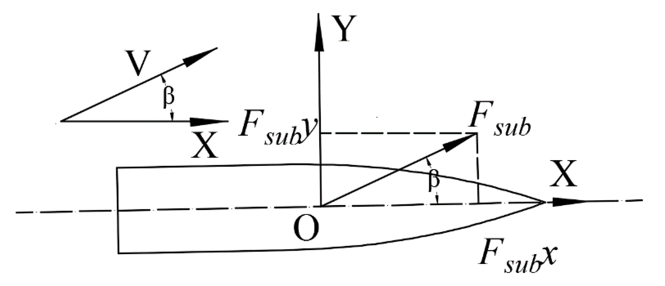
2.2. Calculation of Submersion Forces F_sub

The submersion forces are caused by the rotation or accumulation of broken ice and its sliding along the hull, as shown in Figure 3.

The Lindqvist empirical formula is:

$$R_{ice}=\left(R_c+R_b\right)\left(1+\frac{1.4\nu }{\sqrt{g{H}_{ice}}}\right)+R_s\left(1+\frac{9.4\nu }{\sqrt{gL}}\right)$$

(5)

where R_c is the crushing force; R_b is the bending force, and R_s was assumed as the sum of $R_p$, $R_f$,and $R_{\mu }$; $R_p$ is simplified as the potential energy of ice; $R_f$ is the frictional force of between ice and bow; and $R_{\mu }$ is the frictional force between ice and the ship’s bottom.

$$R_s=R_p+R_f+R_{\mu }$$

(6)

$$R_p={\sigma }_{\rho }g{H}_{ice}B\frac{T\left(B+T\right)}{B+2T}$$

(7)

$$R_f=\mu {\sigma }_{\rho }g{H}_{ice}BT\cos \phi \cos \psi \sqrt{\frac{1}{{\sin }^2\phi }+\frac{1}{{\tan }^2\alpha }}$$

(8)

$$R_{\mu }=\mu {\sigma }_{\rho }g{H}_{ice}B\left(0.7L-\frac{T}{\tan \phi }-\frac{B}{4\tan \alpha }\right)$$

(9)

where δ_ρ is the density difference of ice water, g is the acceleration of gravity, H_ice is the ice thickness, B is the beam, T is the draft, μ is the coefficient of friction, α is the waterline entrance angle, φ is the stem angle, and ψ is the angle between the normal surface and a vertical vector.

When the icebreaker is maneuvering with small and medium drift angles, the submersion forces generated by broken ice are dominated by friction, and the contact area between the broken ice and the hull is close. To calculate the global ice loads in the transversal direction, this paper adopted the approximation in Equation (10) when calculating the submersion forces of the small drift angle maneuvering motion in level ice [18,19,24,41]. Figure 4 gives the schematic diagram of the submersion forces.

$$\{\begin{array}{l}{R}_{sub,x}=R_{sub}\frac{v_x}{\sqrt{v_x^2+v_y^2}}\\ R_{sub,y}=R_{sub}\frac{v_y}{\sqrt{v_x^2+v_y^2}}\end{array}$$

(10)

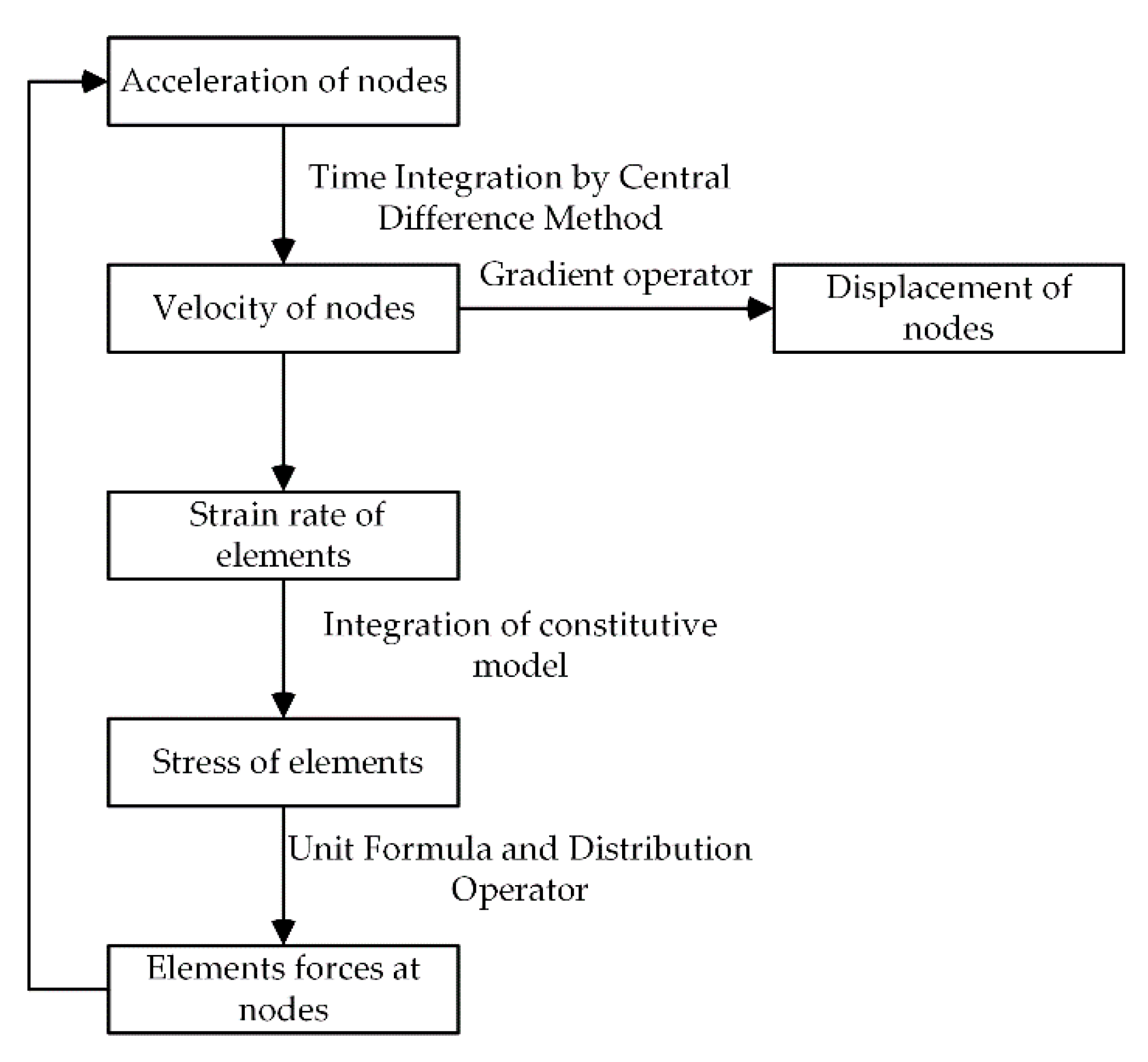
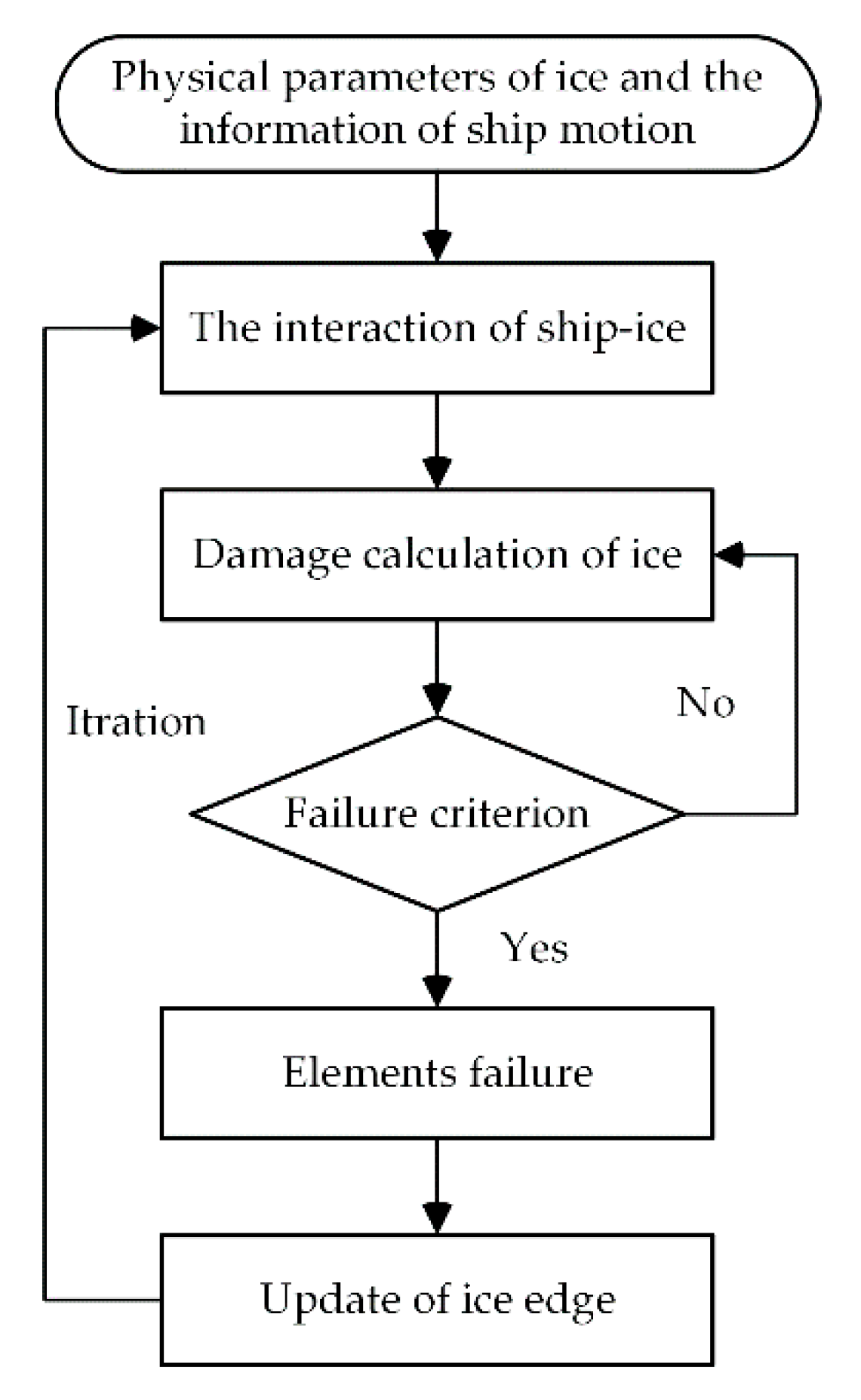
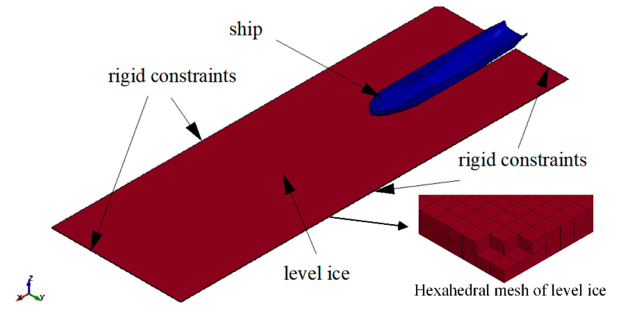
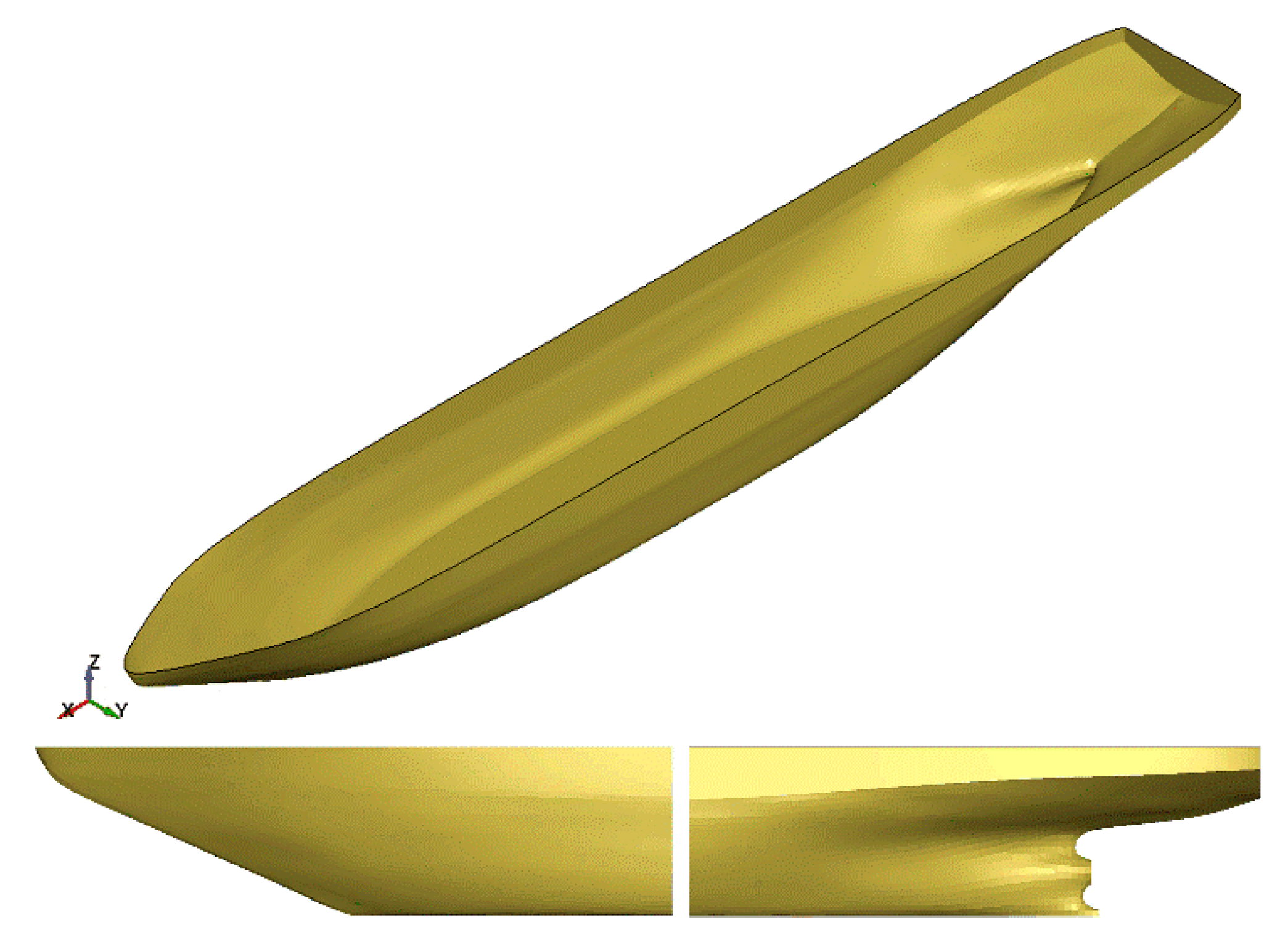
3. Finite Element Numerical Model

This study focused on the global ice loads of the icebreakers, without considering the influences of other environmental loads, and the hull was assumed to be a rigid body. According to the assumption that the icebreakers are located in an infinite navigation field, the boundary of the calculation domain adopted rigid constraints, as shown in Figure 5. The shell and hexahedral solid mesh are used to discretize the hull and level ice, respectively. When the marine structures interact with the level ice, the level ice is usually simplified as a cuboid with uniform thickness, and the same simplification was applied to level ice in our article. For those numerical simulations, the high-quality hexahedral meshes were used to divide the level ice, and all the mesh sizes of ice were the same, as shown in Figure 5. According to the convergence test of mesh size by Subiao [43], the sensitivity analysis of mesh and ice parameters by Long Xue [44], and our [45,46,47] and other researchers’ [48,49] experience in the calculation of global ice loads, to achieve a balance between the computation time and the convergence, the level ice was divided into two layers in thickness, and the mesh sizes were 300 × 500 × 500 mm, 376 × 500 × 500 mm, and 400 × 500 × 500 mm in different cases. The number of meshes and the convergence of the results met the requirements.

Due to the complex material properties of sea ice, a constitutive model of sea ice has not yet been developed. Based on the research of Wang [50] and Liu [51], the isotropic material model with failure of MAT-13 was adopted in the LS-DYNA material library, ignoring the parameters that weaken the strength of sea ice materials, such as porosity, salt degree, etc. The values of density, shear modulus, yield stress, bulk modulus, plastic failure strain, and failure pressure were determined to establish the constitutive model of sea ice (

Table 1. Parameters of sea ice materials in the numerical model.

Parameters	Symbol	Value	Unit
Ice density	ρi	880	kg/m3
Shear modulus	G	2.02	GPa
Bulk modulus	K	5.26	GPa
Failure pressure	Pf	–4	Mpa
Yield stress	σs	2.12	Mpa
Poisson ratio	γ	0.33	-
Frictional coefficient	μi	0.15	-
Plastic failure strain	${\epsilon }_{\max }^p$	0.15	-

). The values of shear modulus and bulk modulus were calculated from the elastic modulus and Poisson’s ratio given in the Araon model test (

Table 2. The values used for the Araon.

Parameters	Symbol	Value	Units
Elastic modulus	E	5.40	Gpa
Compressive strength of ice	σc	2.30	Mpa
Flexural strength of ice	σf	0.55	Mpa
Poisson’s ratio	γ	0.33	-
Frictional coefficient	μi	0.15	-
Gravitational acceleration	g	9.81	m/s2
Ice density	ρi	880	kg/m3
Seawater density	ρw	1024	kg/m3

). Modulus is the ratio of stress and strain under the stress state of the material, and strength is the ability of the material to resist fracture and excessive deformation. Due to the limitation of the numerical method, the modulus parameters of sea ice in numerical simulation and experiment were consistent, but the flexural and compressive strengths were not used as the failure criterion of sea ice, and the minimum pressure and maximum plastic strain were used as the failure criteria of level ice (Equation (11)). When the node satisfies the failure criterion, it will be deleted from FEM to simulate the ice breaking.

$$p^{n+1}<p_{\min } \mathrm{or} {\epsilon }_{eff}^p>{\epsilon }_{\max }^p$$

(11)

where pⁿ⁺¹ is the pressure of the n + 1 step, p_min is the pressure cutoff, ${\epsilon }_{eff}^p$ is the effective plastic strain, and ${\epsilon }_{\max }^p$ is the plastic failure strain.

There are two coordinate systems, the earth coordinate system and the ship coordinate system, to describe the ship’s motion, as shown in Figure 6.

4. Verification of the Numerical Method

Due to the lack of test data, the applicability and accuracy of this method were verified through the literature data on Araon and a multipurpose icebreaker. The main particulars of icebreakers are summarized in

Table 3. Parameters of Araon and multipurpose icebreaker.

Parameters	Multipurpose Icebreaker	Araon	Unit
Lpp	85	93.5	m
B	17	19.0	m
D	6	6.8	m
Waterline entrance angle α	22	54.3	deg
Stem angle φ	25	35.0	deg

, and Figure 7 shows the geometry of Araon and a multipurpose icebreaker.

4.1. Verification of Calculation Method by Icebreaker Araon Model Test

A direct towing model test of Araon was carried out in the KRISO ice tank. The towing speeds were 0.238, 0.357, and 0.476 m/s (2, 3, and 4 knots in full scale) at ice thicknesses of 40.3 mm and 28.7 mm (75.2 cm and 53.4 cm in full scale) [52]. The parameters of the sea ice material are shown in Table 1. Ice tank model tests generally follow Cauchy, Ch, and Froude, Fr, similarity with a full-scall ship (Equation (12)) [53,54]. Therefore, the relationship between full-scale ship ice resistance and model ice resistance is shown in Equation (13), where F_res is the ice resistance of a numerical method and F_res-model is the model test’s ice resistance, which is total resistance minus the open water resistance; the open water resistance, F_ow, of Araon is given in Equation (14) [52]:

$$Fr=\frac{v}{\sqrt{gL}} \mathrm{and} Ch=\frac{v^2\rho }{E}$$

(12)

$$F_{res}={\lambda }^3{F}_{res-model}$$

(13)

$$F_{ow}=13.14V^2,$$

(14)

Figure 8 shows an underwater camera view of the model test and the numerical ice–hull interaction. The model test shows how the bow breaks the level ice into pack ice, which forms accumulation and slides along the bottom of the ship; it should be noted that the numerical simulation is used to simulate ice breaking and F_bre calculation. Figure 8a shows the interaction between level ice and the bow; it can be clearly observed that the level ice was broken into pack ice under the action of the bow. Figure 8b is the bottom view of the interaction phenomena between level ice and the stern. The icebreaking phenomena can still be observed in the stern, but much less than in the bow. Comparing Figure 8a,b, we see that the bow is the main icebreaking structure and the numerical simulation agrees well with the model test phenomena in terms of the breaking of level ice and the width of the channel in direct motion. It is ideal to directly compare the resistance curves obtained from the test and numerical simulation; but due to the limited test data, only the average value of resistance can be used for the verification of the method. The ice resistance predicted by the numerical method and the Araon model test results are shown in Figure 9 and

Table 4. Numerical ice resistance and model test ice resistance, and the deviation of speed of each (λ = 18.667).

Model Test				Full-Scale Ship		Deviation (%)
Model Ship Speed (m/s)	Total Resistance (N)	Open Water Resistance (N)	Ice Resistance (N)	Ice Resistance of Test (KN)	Numerical Ice Resistance (KN)
0.239	116.836	0.745	116.091	755.2	863.3	14.3
0.352	139.634	1.676	137.958	897.3	1055.0	17.6
0.477	171.139	2.980	168.159	1093.8	1195.7	9.4

. The numerical results overestimate the mean ice resistance from the model test: The maximum deviation is 17.6%, the minimum deviation is 9.4%, and the average deviation is 13.8%, which shows good agreement with the Araon model test. The main reason is that the constitutive relation and failure mode of sea ice used in the numerical simulation cannot comprehensively describe the complex material properties of actual sea ice.

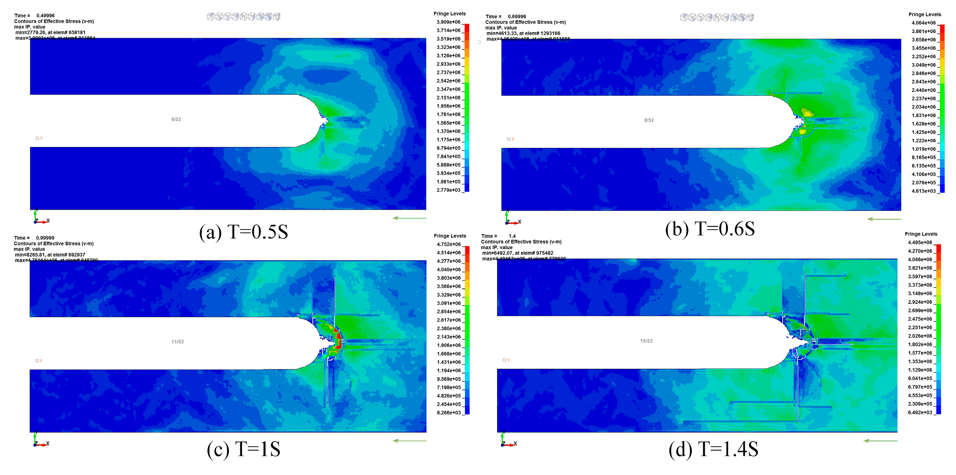
4.2. Analysis of a Typical Direct Motion

The direct motion of the multipurpose icebreaker was simulated with reference to the literature [24] at 11 knots and 0.6-m ice thickness. The main parameters of the icebreaker and ship geometry model are given in Table 3 and Figure 7, respectively. The direct motion can be analyzed from the icebreaking process and mode. Observing the icebreaking resistance curve in Figure 10, there are three peak intervals, whose period is about 1.5 s. The resistance increases rapidly at the beginning of the direct motion and then fluctuates within a certain range.

The specific method of analysis is as follows: (1) At the beginning of the motion, the level ice was squeezed as it collided with the stem, which increased the icebreaking resistance. The first peak of the resistance curve appeared at 0.8 s, and bending of the level ice was observed. (2) After the broken ice fell off, the icebreaking resistance decreased until 1.5 s. (3) As the icebreaker advanced, the stem continued to collide with the level ice and squeeze it, causing the icebreaking resistance to increase again and reach a second peak at 2.3 s. (4) Broken ice started falling off; the icebreaking resistance decreased from 2.5 to 2.9 s. This process repeats continuously during direct sailing, which makes the icebreaking resistance fluctuate within a certain range. The average value of the icebreaking resistance in the peak interval of II and III is 323 KN. According to Equation (10), the submersion resistance is 577 KN, so the ice resistance under this operating condition was about 900 KN. The mean ice resistance was 823 KN in the test.

The study of the icebreaking mode is helpful to understand the icebreaking process under different types of motion. Crushing and bending are the two main modes of icebreaking [24]. The icebreaking modes are mainly related to the shape of the structure. When the level ice collides with a slope structure (such as the stem), the level ice will bend and deform until the stress reaches the flexural strength and the level ice breaks and falls off, as shown in Figure 11a. When the level ice collides with a vertical structure (such as a parallel midship), or the contact area between level ice and a slope structure is too small to bend and break level ice, the breaking of the level ice is mainly via crushing, as shown in Figure 11b.

Figure 12 shows the process of level ice breaking. At the beginning of direct motion, the stem near the waterline began to make contact with the level ice. Meanwhile, the area of contact between the stem and the level ice was too small to break the level ice. Therefore, only crushing was observed in the time interval of 0–0.5 s, as shown in Figure 12a. With the icebreaker’s advance, the contact area between the stem and level ice increased, and the contact force increased as well. At 0.6 s, the level ice began to bend downward, as shown in Figure 12b. Figure 12c shows the bending degree of level ice continuously intensifying from 0.6 s to 1 s, and level ice breakup appeared at 1 s, which can be clearly observed in the red field. The level ice completed bending and fracturing at 1.1–1.5 s, and the broken ice began to fall off, as shown in Figure 12d. In summary, the breaking mode at 0–0.5 s was crushing, and the breaking mode at 0.6–1.5 s was bending, which is in good agreement with the actual icebreaking process shown in Figure 12.

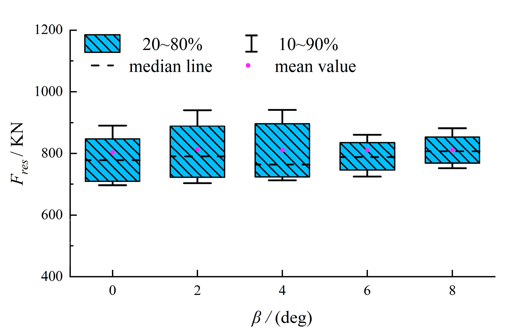
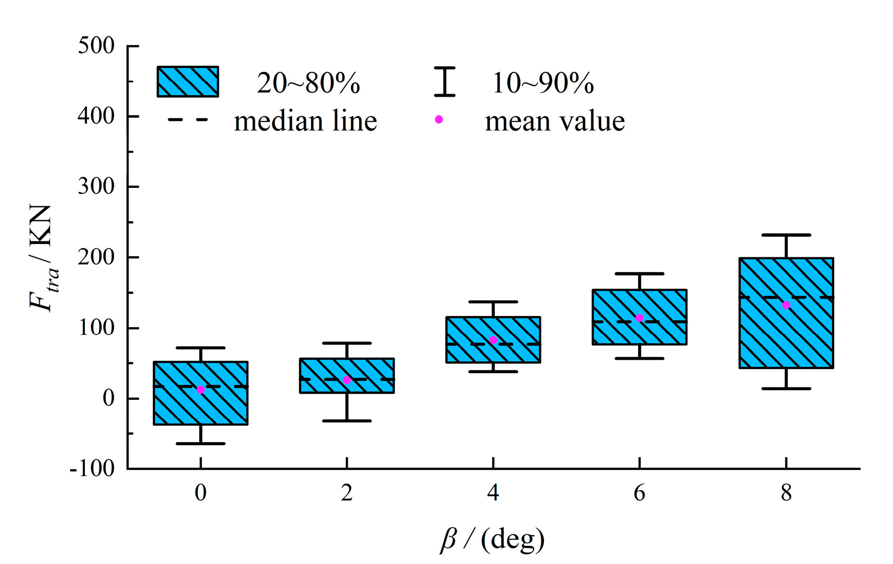
5. Numerical Calculation of Ice Loads in Oblique Motion

Drift angle directly affects the ship–ice interaction area, which determines the distribution of ice loads near the waterline and ultimately determines the global forces on the hull. Therefore, it is worthwhile to research the influence of the drift angle on the ice loads on the hull, which are the factors that directly affect the ship’s maneuverability in the ice [22]. The research on the characteristics of ice loads in maneuvering motion took the icebreaker Xue Long as the research object. The main particulars and geometry of the icebreaker Xue Long are shown in

Table 5. Parameters of the icebreaker Xue Long.

Parameters	Xue Long	Unit
Lpp	147	m
B	22.9	m
D	13.5	m
T	8	m
Waterline entrance angle α	27	deg
Stem angle φ	24	deg

and Figure 13. Considering the effects of small drift angle on ice loads, the oblique motion was simulated at 6 knots of speed, 0.8 m of ice thickness, and five drift angles (from 0 deg to 8 deg). In addition, the computational domain of the numerical model was broadened to 120 m.

Box plots of ice resistance and transverse force are presented in Figure 14 and Figure 15. With the increase in drift angle, the trend of the median line and mean value of ice resistance were not obvious, while those of transverse force increased obviously. This is closely related to the shape and velocity of the icebreaking structure. Ice resistance mainly comes from the icebreaking activity of the stem and the friction of the hull–ice interaction. With the change in drift angle, the velocity in the X-axis and the bow–ice and hull–ice contact area experienced little change, which means the median line and mean value of the box plot showed no obvious change. During oblique sailing, the transverse force mainly comes from vertical structures such as the midship and stern, and the icebreaking ability of the vertical structure is not as good as that of slope structures such as the stem. As the drift angle increases, the midship and stern participate in the icebreaking process, making the transverse force increase continuously.

Figure 16 is a comparison of icebreaking under different drift angles. It shows that the stem is always the main icebreaking structure, but the midship and stern are involved in the process as well. When comparing the level icebreaking of direct and oblique motion, we see that level ice splitting during oblique motion weakens, which is consistent with the model test under different drift angles at the Laboratory of Ice Mechanics and Ice Engineering, Tianjin University [36].

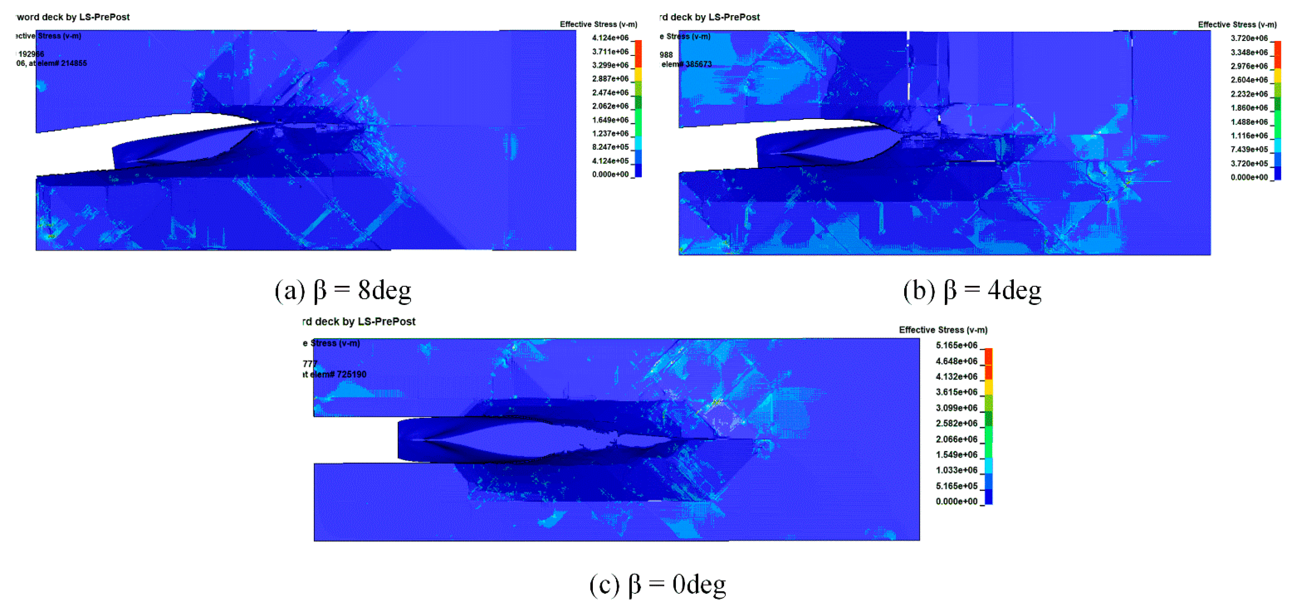
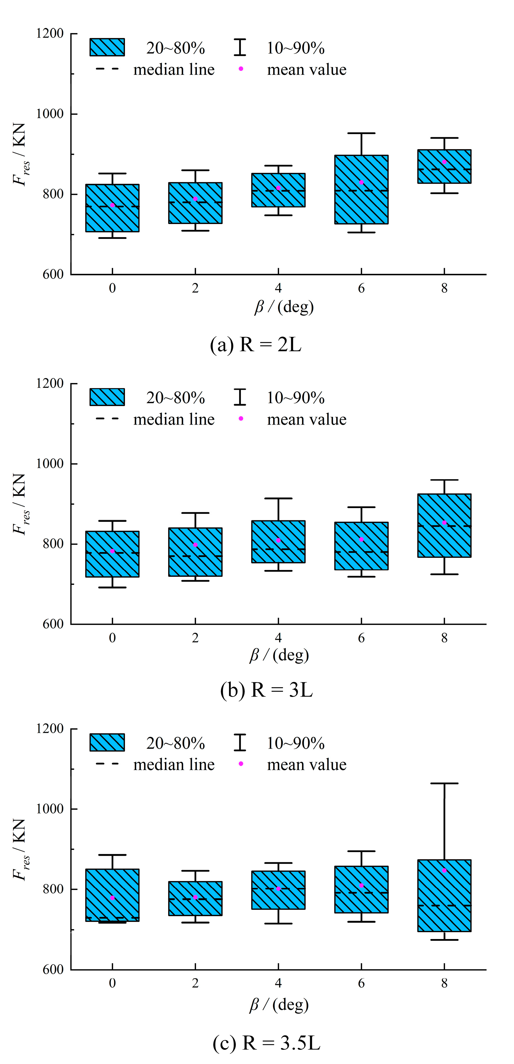
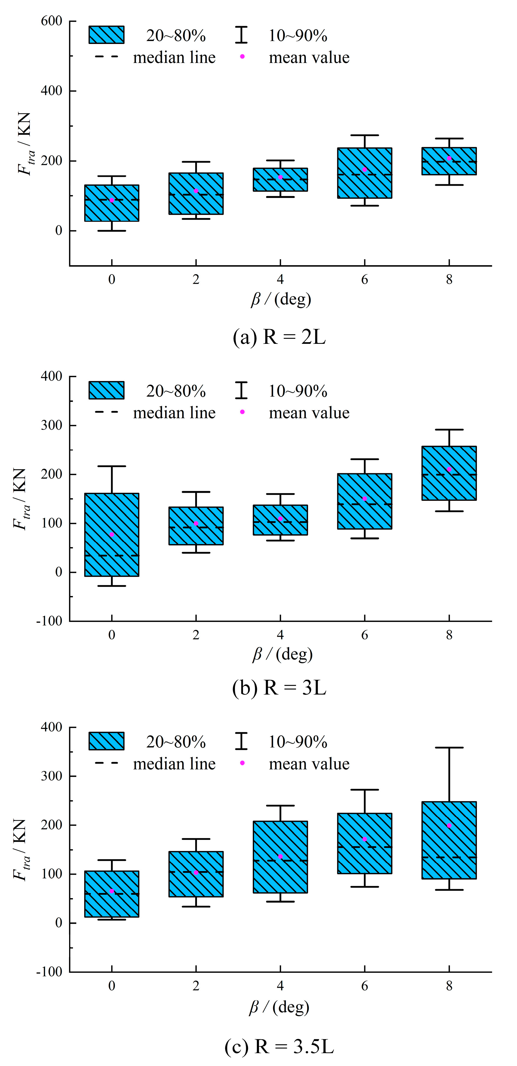
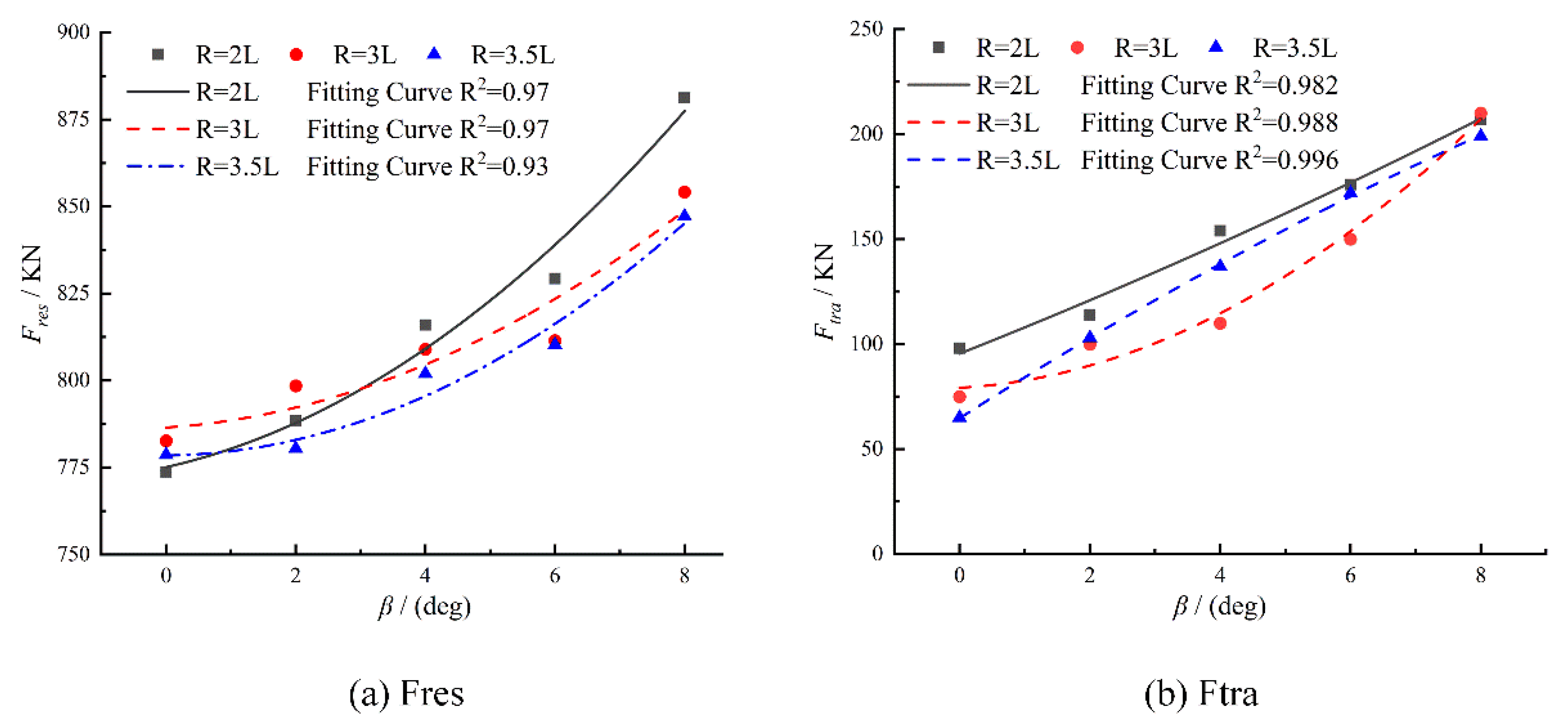
6. Numerical Calculation of Ice Loads in Constant Radius Motion

In a constant-radius maneuver, both drift angle and turning radius will affect the ice–hull interaction area. Hence, a constant radius maneuver was simulated to study the influence of drift angle and turning radii on ice loads at a speed of 6 knots, with 0.8 m of ice thickness. The computational domain width was about 7 B, and the length was 1/8 c round.

Three turning radii (from 2 L to 3.5 L) and five drift angles (from 0 deg to 8 deg) were used in this simulation. Figure 17 and Figure 18 are box plots of ice resistance and transverse force, respectively. When the drift angle increased, the mean value and median line of ice resistance and transverse force increased obviously; the increasing trend of the ice resistance was weaker than that of the transverse force, however. The icebreaker can open up a wider channel with a drift angle, and the stern and midship are involved in the icebreaking process, which leads to the increasing trend of transverse force being greater than that of ice resistance. The effects of drift angle and turning radius are illustrated in Figure 19 and Figure 20. When the turning radius increased, the ice resistance and transverse force had a slight downward trend, but not a very obvious one. This may have been due to the decrease in the angular velocity of the icebreaker, which slowed down the instantaneous ship–ice interaction. Moreover, due to the limited computing resources, the small radius range may be one of the reasons why the trend was not obvious. However, with increasing drift angle, the ice resistance and transverse force both showed an obvious upward trend. It can be seen that the drift angle had a greater impact on the ice loads, which may be related to the effect of drift angle on channel width. National Research Council-Ocean, Coastal and River Engineering (NRC-OCRE) (former National Research Council of Canada-Institute for Ocean Technology, NRC-IOT) carried out a series of planar motion mechanism tests using a 1:21.8-scaled model of Terry Fox, a Canadian icebreaker, in level ice [22]. The numerical results of transverse force showed a trend similar to the model Terry Fox’s test results.

Figure 21 shows the icebreaking process of 5 s, 10 s, 30 s, and 50 s when the turning radius and the drift angle were 3.5 L and 8 deg, respectively. During turning motions, the stern, midship, and stem began to break ice continuously and there was a gap on the starboard side. Figure 22 shows the ice breaking under the drift angles of 0°, 4°, 6°, and 8°. As the drift angle increased, the midship and stern were involved more in the icebreaking process, while the stem was always the main icebreaking structure.

7. Conclusions

The influences of the drift angle and turning radius on the global ice loads of the icebreaker Xue Long were studied based on the widely used combination of numerical simulation and empirical formulas, in which the numerical simulation computes the icebreaking processes and the Lindqvist formula estimates the underwater process. The results are summarized as follows.

First, the accuracy and applicability of the ice load calculation method were verified by the Araon model test of the KRISO ice tank in level ice. The numerical results, mean ice resistance, and icebreaking process were in good agreement with the Araon model test. In addition, the icebreaking process of a multipurpose icebreaker at a higher speed was studied, and the relationship between bending and slope structure, crushing, and vertical structure was discussed. The main mode for slope structures such as the stem is bending; however, the level ice will be crushed under the action of vertical structures, such as ship midships.

Secondly, the influences of drift angle and turning radius on the global ice loads of the icebreaker Xue Long under the maneuvering of the captive oblique and constant radius motion were studied. When the drift angle increased, the variation trend of ice resistance was not obvious, but the ice resistance of the cantilever circular motion increased obviously, and the transverse force of both the constant radius and oblique motion increased. Meanwhile, the transverse force variation of constant-radius motion at different drift angles can be compared with the Terry Fox model test at the NRC/IOT, with which the variation trend of transverse force had a good agreement. The difference in the influence of drift angle on the ice resistance of oblique and constant-radius motion should be related to the rotational angular velocity of the hull. In addition, the splitting of the level ice during oblique motion was reduced compared with the direct motion, which was consistent with the results of the model test in the ice tank of Tianjin University.

There is still limited knowledge about ice load characteristics in level ice, however. Further research should be conducted on establishing more comprehensive sea ice failure criteria and the effects of drift angle and turning radius on local ice loads in terms of maneuvering motion and the effects of high-frequency ice loads on low-frequency maneuvering motions.

References

1. Beveridge, L.; Fournier, M.; Lasserre, F.; Huang, L.; Têtu, P.-L. Interest of Asian shipping companies in navigating the Arctic. Polar Sci. 2016, 10, 404–414. [Google Scholar] [CrossRef]
2. Melia, N.; Haines, K.; Hawkins, E. Sea ice decline and 21st century trans-Arctic shipping routes. Geophys. Res. Lett. 2016, 43, 9720–9728. [Google Scholar] [CrossRef]
3. Kashteljan, V.I.; Poznyak, I.I.; Ryvlin, A.Y. Resistance to Motion of a Ship; Sudostroyeniye: Leningrad, Russia, 1968. [Google Scholar]
4. Shimansky, J.A. Conditional Standards of Ice Qualities of a Ship; Marine Computer Application Corporation: New York, NY, USA, 1969. [Google Scholar]
5. Enkvist, E. On the Ice Resistance Encountered by Ships Operating in the Continuous Mode of Icebreaking; Swedish Academy of Engineering Sciences: Helsinki, Finland, 1972. [Google Scholar]
6. Lindqvist, G. A straightforward method for calculation of ice resistance of ships. In Proceedings of the 10th International Conference on Port and Ocean Engineering under Arctic Conditions (POAC), Luleå, Sweden, 12–16 June 1989; pp. 722–735. [Google Scholar]
7. Lindstrom, C.A. Numerical simulation of ship manoeuvring motion in level ice. In Proceedings of the POLARTECH’90, Copenhagen, Denmark, 14–16 August 1990; pp. 198–208. [Google Scholar]
8. Lindstrom, C.A. Numerical estimation of ice forces acting on inclined structures and ships in level ice. In Proceedings of the Offshore Technology Conference, Houston, TX, USA, 7–10 May 1990. [Google Scholar]
9. Menon, B.; Edgecombe, M.; Tue-fee, K. Maneuvering Tests in Ice aboard Uscgc Polar Star in Antarctica 1985; National Defense Transportation Association: Alexandria, VA, USA, 1986; Volume 46, pp. 30–32. [Google Scholar]
10. Menon, B.; Steele, M.; Samwel, L. Development of a Canadian Arctic Bridge Navigation Simulator: Validation of a Ship-Handling Model; Transportation Development Centre of Transport Canada, Fleet Technology Limited, Arctec Canada Limited: Leggett Drive, ON, Canada, 1988.
11. Menon, B.; Glen, I.; Steele, M.; Hardiman, K. Investigation of Ship Maneuverability in Ice-Phase I; Transport Canada: Ottawa, ON, Canada, 1991.
12. Tue-Fee, K.K.; Keinonen, A.J. Full-scale maneuvering tests in level ice of Canmar Kigoriak and Robert Lemeur. Mar. Technol. SNAME News 1986, 23, 131–138. [Google Scholar] [CrossRef]
13. Tue-Fee, K.K.; Keinonen, A.J.; Menon, B.C. Model for Predicting Steady Turning Performance of Conventional Icebreakers in Level Unbroken Ice. In Proceedings of the International Conference on Ship Manoeuvrability—Prediction and Achievement, Hilton Hotel, London, UK, 29 April–1 May 1987. [Google Scholar]
14. Williams, F.; Spencer, D.; Gagnon, B.; Everard, J.; Butt, S.; Parsons, B.L.; Hackett, P.J.; Institute for Marine Dynamics (Canada). Full-Scale Ice Breaker Trials CCGS Sir John Franklin Indian Arm/Little Burnt Bay 1991; National Research Council Canada: St. John’s, NL, Canada, 1991. [Google Scholar]
15. Williams, F.M.; Waclawek, P. Physical Model Tests for Ship Maneuvering in Ice. In Proceedings of the 25th American Towing Tank Conference, Lowa City, IA, USA, 24–25 September 1998. [Google Scholar]
16. Williams, F.M.; Waclawek, P.; Hyunsoo, K. Simulation of Maneuvering in Ice. In IMD-SAMSUNG Collaborative Project Status Report; Institute for Ocean Technology: St. John’s, NL, Canada, 2006. [Google Scholar]
17. Wang, S. A Dynamic Model for Breaking Pattern of Level Ice by Conical Structures; Helsinki University of Technology: Espoo, Finland, 2001. [Google Scholar]
18. Martio, J. Numerical Simulation of Vessel’s Manoeuvring Performance in Uniform Ice; Helsinki University of Technology Ship Laboratory: Espoo, Finland, 2007. [Google Scholar]
19. Nguyen, D.T.; Sørbø, A.H.; Sørensen, A.J. Modelling and control for dynamic positioned vessels in level ice. IFAC Proc. Vol. 2009, 42, 229–236. [Google Scholar] [CrossRef]
20. Liu, J.; Lau, M.; Williams, F.M. Mathematical modeling of ice-hull interaction for ship maneuvering in ice simulations. In Proceedings of the 7th International Conference and Exhibition on Performance of Ships and Structures in Ice (ICETECH), Banff, AB, Canada, 16–19 July 2006; p. 845. [Google Scholar]
21. Liu, J.; Lau, M.; Williams, M.F. Numerical implementation and benchmark of ice-hull interaction model for ship manoeuvring simulations. In Proceedings of the 19th IAHR International Symposium on Ice, Vancouver, BC, Canada, 6–11 July 2008. [Google Scholar]
22. Liu, J. Mathematical Modeling Ice-Hull Interaction for Real Time Simulations of Ship Manoeuvring in Level Ice; Memorial University of Newfoundland: St. John’s, NL, Canada, 2009. [Google Scholar]
23. Lau, M. Ship manoeuvring-in-ice modeling software OSIS-IHI. In Proceedings of the 21st International Conference on Port and Ocean Engineering Under Arctic Conditions, Montréal, RQ, Canada, 10–14 July 2011. [Google Scholar]
24. Su, B.; Riska, K.; Moan, T. Numerical simulation of ship turning in level ice. In Proceedings of the 29th International Conference on Offshore Mechanics and Arctic Engineering, Shanghai, China, 6–11 June 2010; Volume 4, pp. 751–758. [Google Scholar]
25. Zhou, L.; Su, B.; Riska, K.; Moan, T. Numerical simulation of moored ship in level ice. In Proceedings of the International Conference on Offshore Mechanics and Arctic Engineering, Rotterdam, The Netherlands, 19–24 June 2011; Volume 1, pp. 855–863. [Google Scholar]
26. Tan, X.; Su, B.; Riska, K.; Moan, T. A six-degrees-of-freedom numerical model for level ice–ship interaction. Cold Reg. Sci. Technol. 2013, 92, 1–16. [Google Scholar] [CrossRef]
27. Zhou, Q.; Peng, H. Numerical simulation of a dynamically controlled ship in level ice. Int. J. Offshore Polar Eng. 2014, 24, 184–191. [Google Scholar]
28. Riska, K. Performance of Merchant Vessels in Ice in the Baltic; Sjöfartsverket: Luleå, Sweden, 1997.
29. Vance, G.P. Analysis of the Performance of a 140-Foot Great Lakes Icebreaker: USCGC Katmai Bay; Cold Regions Research and Engineering Laboratory: Hanover, NH, USA, 1980. [Google Scholar]
30. Zhou, L.; Riska, K.; Von Bock und Polach, R.U.F.; Moan, T.; Su, B. Experiments on level ice loading on an icebreaking tanker with different ice drift angles. Cold Reg. Sci. Technol. 2013, 85, 79–93. [Google Scholar]
31. Zhou, L.; Chuang, Z.; Ji, C. Ice forces acting on towed ship in level ice with straight drift. Part I: Analysis of model test data. Int. J. Nav. Archit. Ocean. Eng. 2018, 10, 60–68. [Google Scholar] [CrossRef]
32. Zhou, L.; Chuang, Z.; Bai, X. Ice forces acting on towed ship in level ice with straight drift. Part II: Numerical simulation. Int. J. Nav. Archit. Ocean. Eng. 2018, 10, 119–128. [Google Scholar] [CrossRef]
33. Derradji-Aount, A.; Thiel, A. Terry Fox Resistance Tests-Phase Ⅲ (PMM) Testing ITTC Experimental Uncertainty Analysis Initiative; Institute for Ocean Technology: St. John’s, NL, Canada, 2004. [Google Scholar]
34. Derradji-Aount, A.; Izumiyama, K.; Yamaguchi, H.; Wilkman, G. Experimental Uncertainty Analysis for Ice Tank Ship Resistance Experiments Using a Model for a Canadian Icebreaker Terry Fox. Ocean. Eng. Int. 2004, 8, 49–68. [Google Scholar]
35. Spencer, D.S.; Timco, G.W. CD model ice—A process to produce correct density (CD) model ice. In Proceedings of the 10th International IAHR Symposium on Ice, Espoo, Finland, 23–27 August 1993; Volume 2, pp. 745–755. [Google Scholar]
36. Wu, W. Model Tests on Ice Resistance of an Icebreaking Ships with Different Ice Drift Angles; Tianjin University: Tianjin, China, 2017. [Google Scholar]
37. Lau, M. Discrete element modeling of ship manoeuvring in ice. In Proceedings of the 18th International Symposium on Ice, Sapporo, Japan, 28 August–1 September 2006. [Google Scholar]
38. Zhan, D.; Agar, D.; He, M.; Spencer, D.; Molyneux, D. Numerical simulation of ship maneuvering in pack ice. In Proceedings of the International Conference on Offshore Mechanics and Arctic Engineering, Shanghai, China, 6–11 June 2010; pp. 855–862. [Google Scholar]
39. Zhan, D.; Molyneux, D. 3-dimensional numerical simulation of ship motion in pack ice. In Proceedings of the International Conference on Offshore Mechanics and Arctic Engineering, Rio de Janeiro, Brazil, 1–6 July 2012; Volume 6, pp. 407–414. [Google Scholar]
40. Li, F.; Kotilainen, M.; Goerlandt, F.; Kujala, P. An extended ice failure model to improve the fidelity of icebreaking pattern in numerical simulation of ship performance in level ice. Ocean. Eng. 2019, 176, 169–183. [Google Scholar] [CrossRef]
41. Li, F.; Goerlandt, F.; Kujala, P. Numerical simulation of ship performance in level ice: A framework and a model. Appl. Ocean. Res. 2020, 102, 102288. [Google Scholar] [CrossRef]
42. Hajivand, A.; Mousavizadegan, S.H. Virtual simulation of maneuvering captive tests for a surface vessel. Int. J. Nav. Archit. Ocean. Eng. 2015, 7, 848–872. [Google Scholar] [CrossRef] [Green Version]
43. Su, B. Numerical Predictions of Global and Local Ice Loads on Ships; Norwegian University of Science and Technology: Trondheim, Norway, 2011. [Google Scholar]
44. Long, X. Discrete Element Analysis of Sea Ice Failure Mode and Ice Load during the Interaction with Marine Structure; Dalian University of Technology: Dalian, China, 2019. [Google Scholar]
45. Xuan, S. Numerical Calculation of Ship Maneuvering Ice Load in Level Ice; Wuhan University of Technology: Wuhan, China, 2019. [Google Scholar]
46. Hu, X. The Numerical Simulation of Ship Icebreaking and Navigating Based on FEM-SPH Coupling Algorithm; Wuhan University of Technology: Wuhan, China, 2016. [Google Scholar]
47. Hu, X.; Zhan, C.S. Numerical simulation of ship ice breaking based on FEM-SPH coupling algorithm. JiangSu Ship 2015, 32, 9–13. [Google Scholar]
48. Teng, M. Caculation and Numerical Simulation of the Ice Load on the Icebreaker; Harbin Engineering University: Harbin, China, 2014. [Google Scholar]
49. Zhai, S. A Method for Numerical Simulation of the Icebreaker in the Process of Icebreaking; Harbin Engineering University: Harbin, China, 2014. [Google Scholar]
50. Wang, J. Numerical Study on Ship Collision with Level Ice Based on Nonlinear Finite Element Method; Shanghai Jiao Tong University: Shanghai, China, 2015. [Google Scholar]
51. Liu, Y. Study on the Structural Strength Evaluation and Optimization Design Method of the Ice Belt of the Polar Warship; Harbin Engineering University: Harbin, China, 2018. [Google Scholar]
52. Jeong, S.-Y.; Choi, K.; Kang, K.-J.; Ha, J.-S. Prediction of ship resistance in level ice based on empirical approach. Int. J. Nav. Archit. Ocean. Eng. 2017, 9, 613–623. [Google Scholar] [CrossRef]
53. Ashton, G.D. River and Lake Ice Engineering; Water Resources Publication: Littleton, CO, USA, 1986. [Google Scholar]
54. Huang, Y.; Shi, Q.Z.; Song, A. The study of the scaling law in dynamic ice force model tests. China Offshore Oil Gas 2007, 6, 419–423. [Google Scholar]
Figure 1. Flow chart of each time step.
Jmse 09 01404 g001
Figure 2. The solution process of ship–ice interaction.
Jmse 09 01404 g002
Figure 3. The motion of broken ice in a test.
Jmse 09 01404 g003
Figure 4. A schematic diagram of submersion forces. Fsub is the submersion force, Fsubx is the component of the submersion force on the X-axis, Fsuby is the component of the submersion force on the Y-axis, V is the ship speed, vx is the X component of the velocity, and vy is the Y component of the velocity.
Jmse 09 01404 g004
Figure 5. Computational domain and boundary conditions.
Jmse 09 01404 g005
Figure 6. Schematic diagram of the coordinate system.
Jmse 09 01404 g006
Figure 7. Ship geometry model.
Jmse 09 01404 g007
Figure 8. Two underwater views of the ice–hull interaction. (a) Bow; (b) stern.
Jmse 09 01404 g008
Figure 9. Comparison of numerical results and model test data for the icebreaker Araon.
Jmse 09 01404 g009
Figure 10. Icebreaking resistance curve.
Jmse 09 01404 g010
Figure 11. Breaking mode of level ice (www.eworldship.com, accessed on 19 July 2014).
Jmse 09 01404 g011
Figure 12. Icebreaking in peak interval Ⅰ.
Jmse 09 01404 g012
Figure 13. The geometry of the icebreaker Xue Long.
Jmse 09 01404 g013
Figure 14. Box plot of Fres under different drift angles.
Jmse 09 01404 g014
Figure 15. Box plot of Ftra under different drift angles.
Jmse 09 01404 g015
Figure 16. Comparison of icebreaking under different drift angles.
Jmse 09 01404 g016
Figure 17. Box plot of Fres under different drift angles.
Jmse 09 01404 g017
Figure 18. Box plot of Ftra under different drift angles.
Jmse 09 01404 g018
Figure 19. Average ice resistance and transverse force curves under different drift angles.
Jmse 09 01404 g019
Figure 20. Average ice resistance and transverse force curves under different turning radius.
Jmse 09 01404 g020
Figure 21. Comparison of ice breaking at different times (3.5 L, β = 8°).
Jmse 09 01404 g021
Figure 22. Comparison of ice breaking under different drift angles (3.5 L).
Jmse 09 01404 g022