Article

Study on Slamming Pressure Characteristics of Platform under Freak Wave

1
School of Naval Architecture and Ocean Engineering, Jiangsu University of Science and Technology, Zhenjiang 212028, China
2
School of Marine Engineering and Technology, Sun Yat-Sen University, Zhuhai 519082, China
*
Author to whom correspondence should be addressed.
J. Mar. Sci. Eng. 2021, 9(11), 1266; https://doi.org/10.3390/jmse9111266
Submission received: 12 October 2021 / Revised: 3 November 2021 / Accepted: 9 November 2021 / Published: 13 November 2021
(This article belongs to the Special Issue Ship Motions and Wave Loads)

Abstract

:
Freak waves have great peak energy, short duration, great contingency, and strong nonlinear characteristics, and can cause severe damage to ships and marine structures. In this study, numerical simulations in conjunction with experimental tests are applied to study air gap response and wave slamming loads of a semi-submersible offshore platform under a freak wave. A three-dimensional wave tank, which is created based on the computational fluid dynamics (CFD) method, is applied to study the hydrodynamic responses of a semi-submersible platform. The numerical model of the tank and offshore platform system are checked according to the experimental results. A typical freak wave is modelled in numerical wave tanks by the linear superposition method, and its significant wave height is 13.03 m. It is found that the freak wave is closely associated with the wave slamming. The appearance of the freak wave gives rise to a negative air, gap which appears on the side of the back wave surface at the bottom of the deck box, and considerable slamming pressure is generated. Furthermore, the wave run up at the junction of the column and the buoyancy tank is also seen due to the freak wave.

1. Introduction

In recent decades, waves and tides [1] have been studied extensively, including the movement of material by the sea and the effect of wave action on structures. Much maritime distress indicates that freak waves cause severe damages to ocean platforms. The generation mechanism of freak waves and their interactions with floating structures have been well studied by numerical simulations or experimental methods in previous researches. However, there is no mature theory to explain nonlinearity and energy concentration characteristics caused by freak waves. Generalized wave slamming is also validated for wave slamming due to freak waves. In previous numerical simulations, the potential flow theory and Morrison equation were mainly used. Baarholm et al. [2] used three numerical methods to solve the boundary value problem and obtained the slamming pressure expression at the bottom of the deck of a fixed offshore platform. Jiang et al. [3] analyzed the wave loads of floating offshore platforms based on the potential flow theory. The variation of wave loads on floating offshore platform under different environmental conditions was obtained. Unfortunately, the potential flow theory neglects the viscosity of water, and the wave slamming problem with strong nonlinearity needs to be further studied. Zhang et al. [4] present a numerical study of the impact of a two-dimensional plunging wave on a rigid vertical wall in the context of potential flow, but the slamming characteristics of complex three-dimensional moving structures are obviously different from them. Faltinsen [5] and Jain [6] proposed a classical model to approximate the interaction between small amplitude regular waves and simple structures. However, the accuracy of the traditional simplified model was significantly reduced as the physical size of the model and the complexity of the structural configuration increased. Therefore, Nielsen [7] applied the integral boundary method to improve the accuracy of numerical simulations, and it was pointed out that it is able to preliminarily deal with wave slamming on complex models. At the same time, large-scale model tests are becoming popular methods in studying wave thumping. Liu et al. [8] reviewed the slamming pressure of a semi-submersible platform in different waves by the model test method. They found that the slamming pressure and frequency were the most serious in the quartering sea wave condition, which was followed by the head sea wave condition, and were relatively mild in the oblique wave environment. Huo [9] conducted nonlinear numerical simulations on the slamming frequency and slamming load of a semi-submersible platform.
The air gap is one of the important concerns during the design procedure of offshore platforms. As a classical theory of fluid mechanics, potential flow theory was widely adopted in investigating the air gap of offshore platform due to its high efficiency. A numerical simulation in conjunction with experimental tests was applied to analyze the air gap response. Simos et al. [10] carried out model tests to study hydrodynamic responses of a semi-submersible platform, and it was found that the run up of wave near the column was often ignored in previous studies. Lwanowski et al. [11] used Com Flow software to analyze the air gap of an offshore platform and compared the numerical results with the experimental ones. Li et al. [12] studied air gap responses of a semi-submersible platform under severe environmental conditions.
A detailed study of the freak wave generation mechanism needs to be investigated to understand the freak wave slamming phenomenon more comprehensively. Generally, the modelling theory of freak waves can be divided into two categories: linear and nonlinear models. Compared to more computationally complex and nonlinear models, the linear superposition model (Longuet-Higgins wave model) [13] has been studied more extensively, and it has been successfully applied to generate freak waves. Deng et al. [14] and Alexander I. Dyachenko et al. [15] used nonlinear models to generate freak waves. These models deal with freak waves as a superposition of a series of waves with different frequencies and phases. Distortional waves can be generated at specific times and spaces by using appropriate models. Zhang et al. [16] and Gao et al. [17] used a linear superposition model to generate freak waves. Because of the tremendous wave height, swift propagation speed, and extremely destructive characteristics of freak waves, it is important to study the safety of marine structures under the attack of freak waves. Huang et al. [18] generated a freak wave at specific times and positions by combining 100 groups of cosine waves, and the results were compared with experimental results. Zhang et al. [19] generated freak waves by utilizing wave superposition theory. They studied the effect of freak waves on motions of a rigid plate and the slamming pressure. The local slamming pressure distribution of rigid plate subjected to freak wave slamming was obtained. Based on the improved double wave train superposition model of the Longuet-Higgins’s theory, Zhang et al. [20] carried out numerical simulation to study freak waves. Wei et al. [21] constructed model tests on wave load characteristics of an inward capsized ship under a freak wave. Based on the linear wave superposition theory, a freak wave was generated in a towing tank. To investigate the influence of ship speed on wave load, model tests of an inward capsized ship under a freak wave were carried out. In addition, compared with regular waves, many waveforms have different effects on the hull. Peregrine DH [22] concluded that the more violent impacts of water waves on walls create velocities and pressures having magnitudes much larger than those associated with the propagation of ordinary waves under gravity. CLAUSE G et al. [23] described techniques to synthesize nonlinear gravity waves in irregular seas. Extreme waves registered in nature were simulated in a physical wave tank. Furthermore, the impact of the New Year Wave on a semi-submersible and two stationary ships was investigated.
In this study, the air gap response to motion and wave slamming characteristics of offshore platform under freak wave are studied by combining numerical simulation with experimental tests. A typical freak wave is built in the numerical tank based on CFD by the method of linear superposition. The air gap response to motion and slamming pressure distribution characteristics of the platform under the effect of a freak wave is studied, which provide a reference for the platform design under freak wave. This study is organized as follows: a theoretical study on numerical wave tanks, the establishment and verification of a numerical model, and a study on the load distribution of a platform under a freak wave in numerical simulation.

2. Theoretical Study on Numerical Wave Tanks

2.1. Governing Equations and Discrete Methods

The mathematical model of numerical wave tank consists of continuity equation and N-S equation:
ρ t + ( ρ u i ) x i = 0 ( i , j = 1 , 2 , 3 )
( ρ u i ) t + ( ρ u i u j ) x i = x j [ μ ( u i x j + u j x i ) ] p x i + ρ f i ( i , j = 1 , 2 , 3 )
where ρ is the fluid density, p is fluid pressure, μ is the dynamic viscosity coefficient, fi is mass force, ui is the velocity component of fluid particle in i direction, and t is time.
In this paper, the K-ω turbulence model is selected, and the governing equation of the flow field is discretized by the finite volume method. The convection term and the diffusion term are discretized by the second-order upwind scheme. Finally, the SIMPLE algorithm is used to correct the pressure field and velocity field.

2.2. Free Surface Tracking Method

For tracking the free wave surface, the volume of fluid method is used for processing. VOF method is mainly used to determine the shape and position of the free surface by the ratio function of the fluid volume in the grid cell and the total volume of the grid. The equation is:
a q t + ( u i a q ) x i = 0 ( q = 1 , 2 )
where a1 and a2 are the volume fraction of air and water phase, respectively. The free wave surface aq is 0.5.
When using this method to capture the free surface, it is necessary to reconstruct the interface to process the fuzzy interface for the second time to ensure the accuracy of the results.

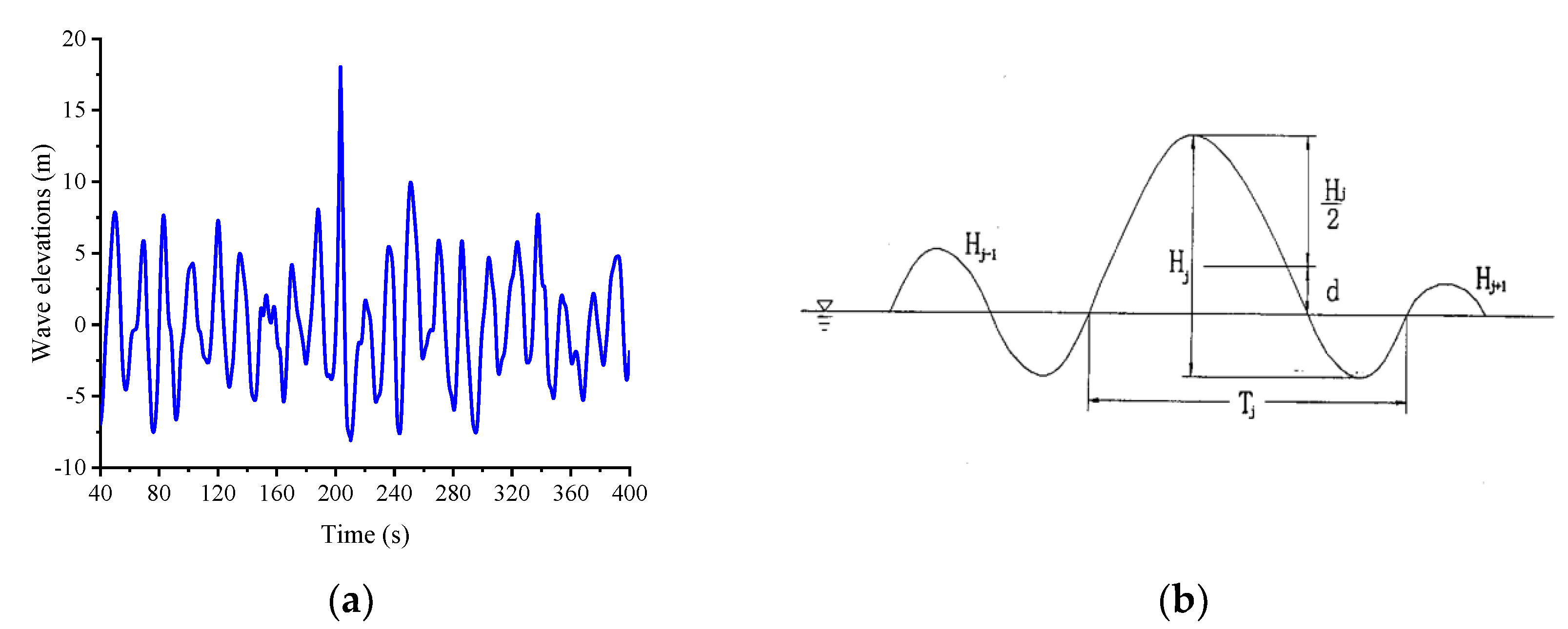
2.3. Numerical Wave Making Theory of Freak Wave

According to the current academic requirements, the determination of freak waves should meet the following three conditions:
(1)
The maximum wave height of a freak wave is not less than twice as much as the significant wave height;
(2)
The maximum wave height of the freak wave is greater than twice the height of the adjacent wave;
(3)
The ratio of the peak to the height of the freak wave is about 0.65.
The wave train superposition model for freak wave simulation is defined as follows:
η ( x , t ) = 1 M a i cos ( k i x + ω i t + ε i )
Generally, the value of x is zero, and the above formula is simplified as:
η ( x , t ) = 1 M a i cos ( ω i t + ε i )
ω i ω i + Δ ω 1 2 a i 2 = S ( ω i ) Δ ω
where M is the number of waves. ai and ωi are the amplitude and frequency of the i-th wave, respectively. εi is the initial phase of the i-th wave, which is randomly selected in the range of (0, 2π). Δω is the frequency difference, and η(x,t) is the wave height of each wave. S(ωi) is the wave spectral density function.
To obtain more accurate wave elevations, a correction function is introduced to revise the wave elevations obtained in the above expression:
η ( x , t ) = 2 20 a i cos ( k i ( x x c ) + ω i ( t t c ) + ε i ) + a m a 1 cos [ k ( x x c ) + ( β m ω 1 ) ( t t c ) ]
ω i ω i + Δ ω 1 2 a i 2 = S ( ω i ) Δ ω
S ( ω i ) = 0.008 g 2 ω i 5 exp ( 0.74 g 4 u 19.5 4 ω i 4 )
u 19.5 = 6.85 H s
ω i 2 = k i × g × th k d
where in Formula (7), the selected target spectrum type is P-M, and αm and βm are correction coefficients. When αm is 25.12 and βm is 4.43 [13], the correction effect is the best. In deepwater, thkd is approximately equal to the 1, ωi2 is the product of ki, and g. u19.5 is the wind speed from the sea surface to the height of 19.5 m. g is the acceleration of gravity, tc is the occurrence time of freak wave, and xc is the location of freak wave.

2.4. Numerical Wave Making Method of Freak Wave

The linear superposition method is a conventional method used in wave tanks as well as in numerical wave tanks. The generation method for freak waves in this study is based on the classical Longuet-Higgins model, which linearly superposes 20 different cosine waves. The wave period and wave height of these 20 cosine waves are shown in Table 1, where H is the wave height and T denotes the wave period. In order to make waveform satisfy the definition of freak wave in a shorter wave train as far as possible, the initial phase is set as zero for all cosine waves. The cuboid computing domain is adopted. The distance between the entrance and exit of the computational domain and the centroid is set as 210 m and 280 m, respectively. The length of the wave elimination region is set as 1.4 times the wavelength. The free surface is meshed by prism layer, and the part outside the free surface is meshed by cutting body.
Figure 1 shows the superposition of 20 cosine waves by numerical simulation. The maximum wave height of the freak wave is 26.2 m, and the significant wave height is 13.03 m. The ratio of the maximum wave height to the significant wave height is greater than 2.0. The ratios of the maximum wave height to the adjacent wave heights are 2.05 and 3.47, respectively. The peak wave height is 18.04 m, and the ratio of the freak wave crest to wave trough μ is 0.696. The above three results verify that the superposition model is accurate enough, which is beneficial to the numerical simulation of freak waves and the study of wave slamming of platforms under freak wave.

3. Establishment and Verification of Numerical Model

3.1. Selection of Similarity Ratio

Bulleted lists look like this: a double buoyancy tank semi-submersible platform is studied. In the numerical simulation, the smaller primary mesh size can present more accurate estimations to the flow field and the motion responses of floating body. A large-scale ratio will affect the size of grid, which is easy to give rise to wave attenuation, motion distortion, and so on. However, the number of grids increases significantly with the decrease of scale ratio, which would result in redundant computing costs. Considering the conditions of the numerical simulation, the ratio of 1:20 is used in this study.
It is necessary to determine the size of the model structure before model tests. To simulate the physical mechanisms and hydrodynamic properties of fluids, model test and the prototype must follow three principles, including geometric similarity, kinematic similarity and dynamic similarity. Considering the cost of computation time, the capacity of wave maker, and the size of tank, the model scale is determined as 1:100 in this study.

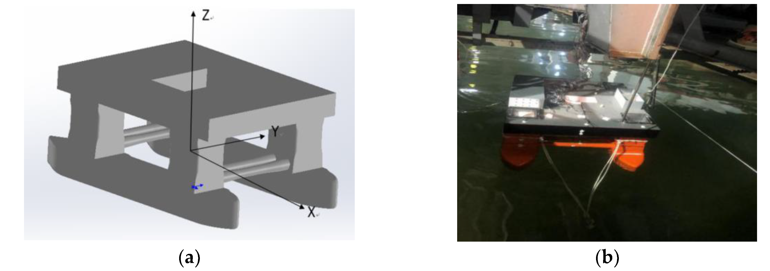
3.2. Description of the Platform Model

Experimental tests were conducted in the wave basin of Jiangsu University of Science and Technology (38 m long, 15 m wide, and 1 m deep). A piston wave generator was installed on one end of the basin to generate incident waves, and on the opposite end of wave generator a wave-absorbing beach was installed to reduce reflected waves. When the wave reached the end of the tank, the wave climbed, along with the wave-eliminating equipment. The wave was then crushed by the wave-eliminating gravel. A large amount of wave energy was consumed, thereby effectively suppressing the residual wave. In addition, since the ratio of the experimental water depth (1 m) to the draft (0.155 m) was greater than 4, the shallow water effect can be ignored.
The numerical and experimental models are shown in Figure 2. The origin of the coordinates was defined at the centroid of the overall structure. The main dimensions and hydrostatic parameters of the platform are shown in Table 2 and Table 3, respectively.

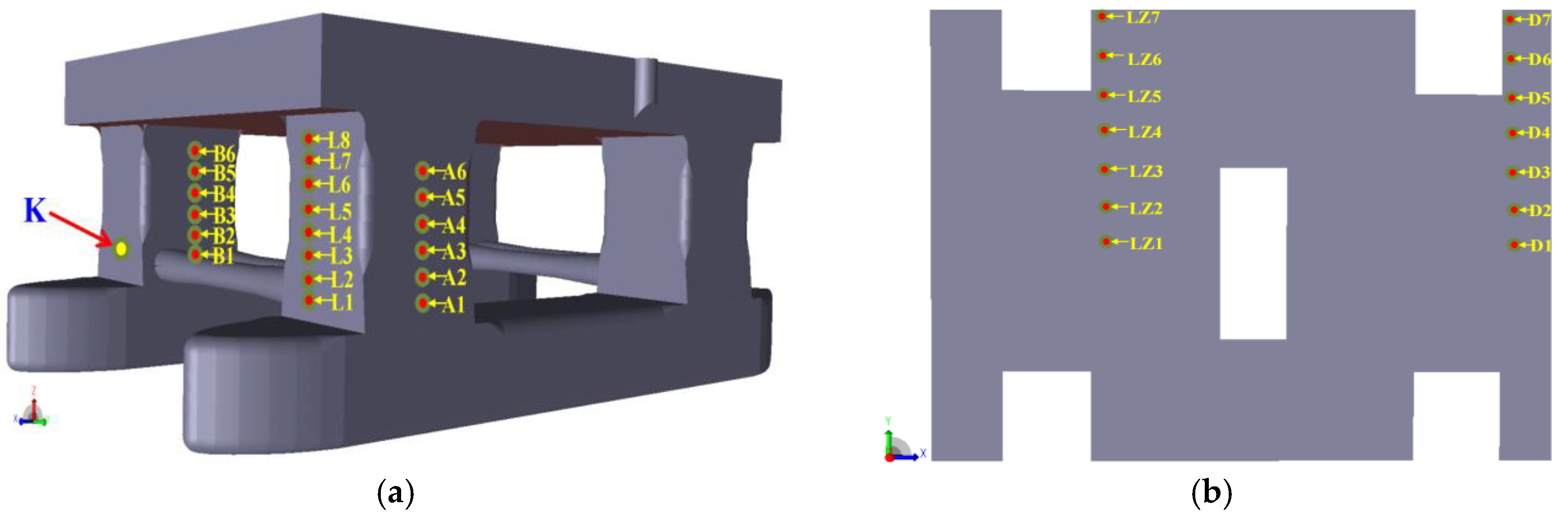
3.3. Platform Monitoring Point Location

Figure 3 shows the distribution of monitoring points on the semi-submersible platform. The thump pressure monitoring points on the lower surface of the semi-submersible platform riser and upper deck are marked as L1–L8, A1–A6, B1–B6, D1–D7, and LZ1–LZ7. The coordinates of the monitoring points are shown in Table 4. The middle and lower positions of the front surface of the column are vulnerable to wave slamming.
As can be seen in Figure 3, L1–L8 are set uniformly on the surface of the columns of the numerical model to investigate the wave slamming loads on the column along with height, and the distance between each two monitoring points is 2 m. Among them, L8 is located on the junction of the buoyancy tank and the column. A1–A6 are monitoring points on the front column, and B1–B6 are arranged on the rear column. The vertical distance between A1 and A6 is 3 m. A1–A6 and B1–B6 are used to analyze the wave slamming in beam sea. In addition, the bottom of the upper deck is a position that is often subjected to the wave slamming. Therefore, the slamming load on the bottom of the upper deck should be calculated. D1–D7 and LZ1–LZ7 are placed on the front and rear vertical columns to the center line of the deck, respectively, with an equal distance of 6 m.
To further verify the numerical model, the numerical pressure slamming of K-point at the midline of the vertical surface of the column is compared with the numerical one.

3.4. Verification of Numerical Model

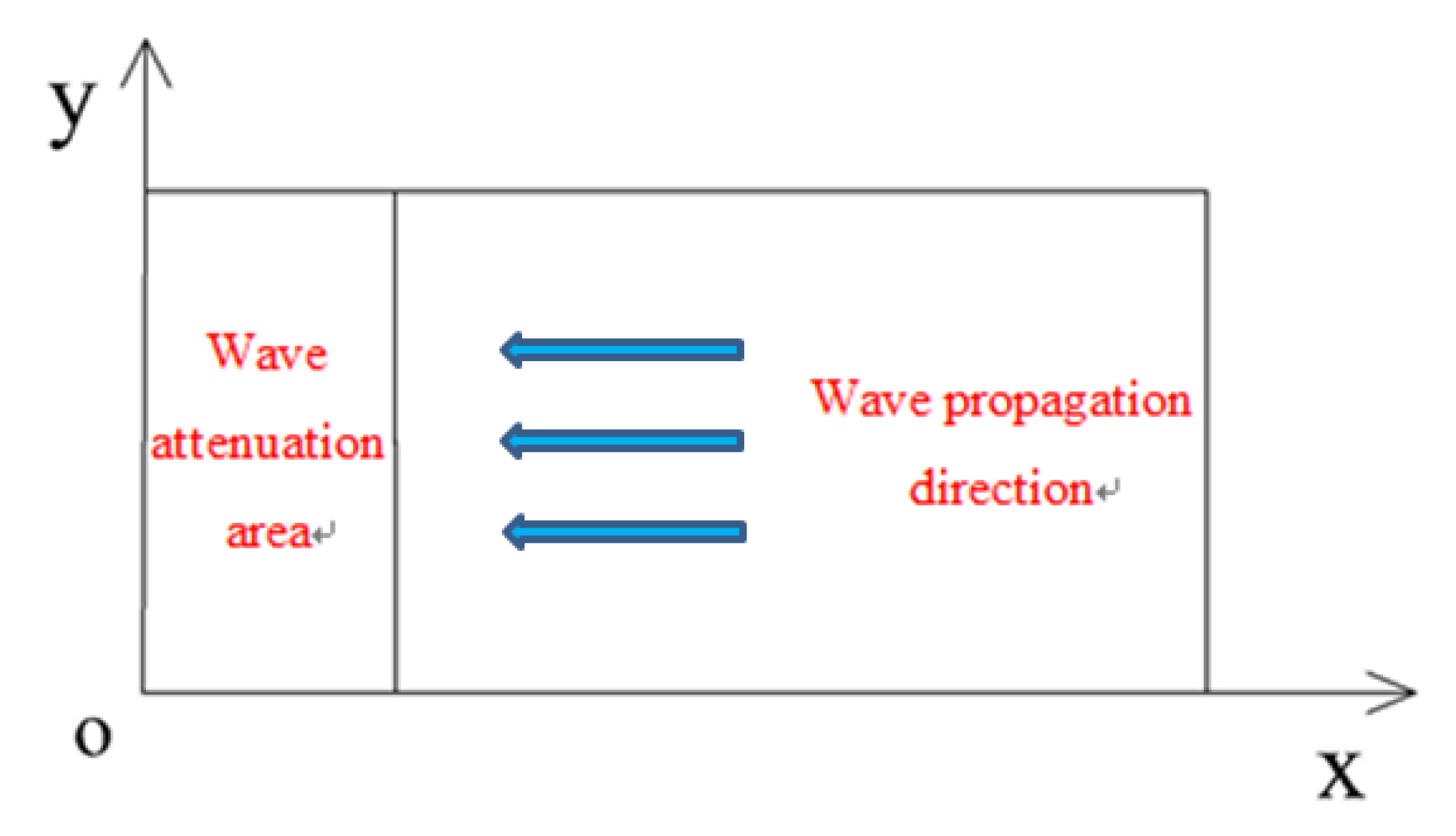
3.4.1. Wave Making and Wave Elimination of Numerical Tank

The accuracy of the numerically simulated waves should be verified before the calculation of slamming loads. In this study, the boundary wave making method is adopted. The velocity and wave surface expressions of the air and water phase are defined at the entrance boundary. The water surface is captured by the fluid volume function method (VOF). The wave is a linear micro amplitude wave based on the fifth-order linear wave theory. Dong et al. [24] claimed that the wave energy density of the fifth-order Stokes is more consistent with the numerical integration result, compared with other wave models.
Damping dissipation regions are installed at the outlet and both walls of the tank to improve the stability of the wavefield in this area. In this study, the length of the wave elimination area is set as 1.5 times the wavelength. The schematic of the wave elimination region is shown in Figure 4.

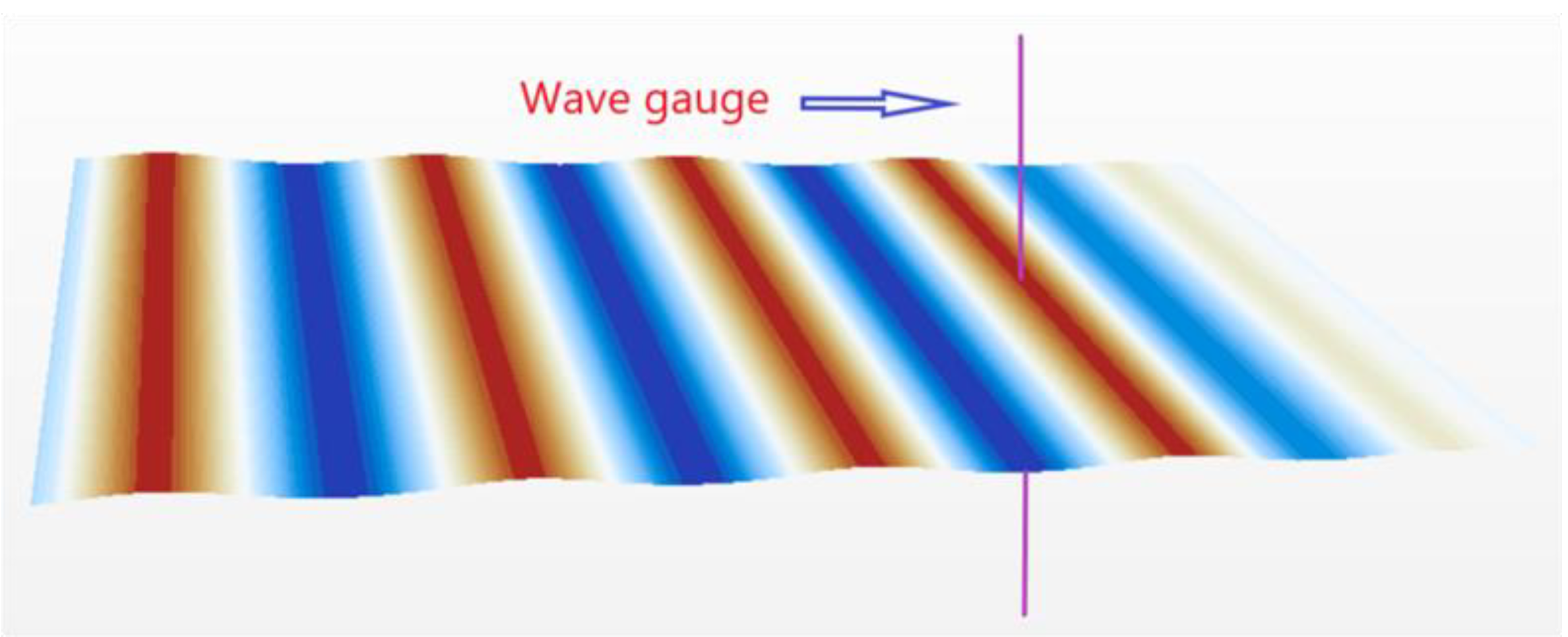
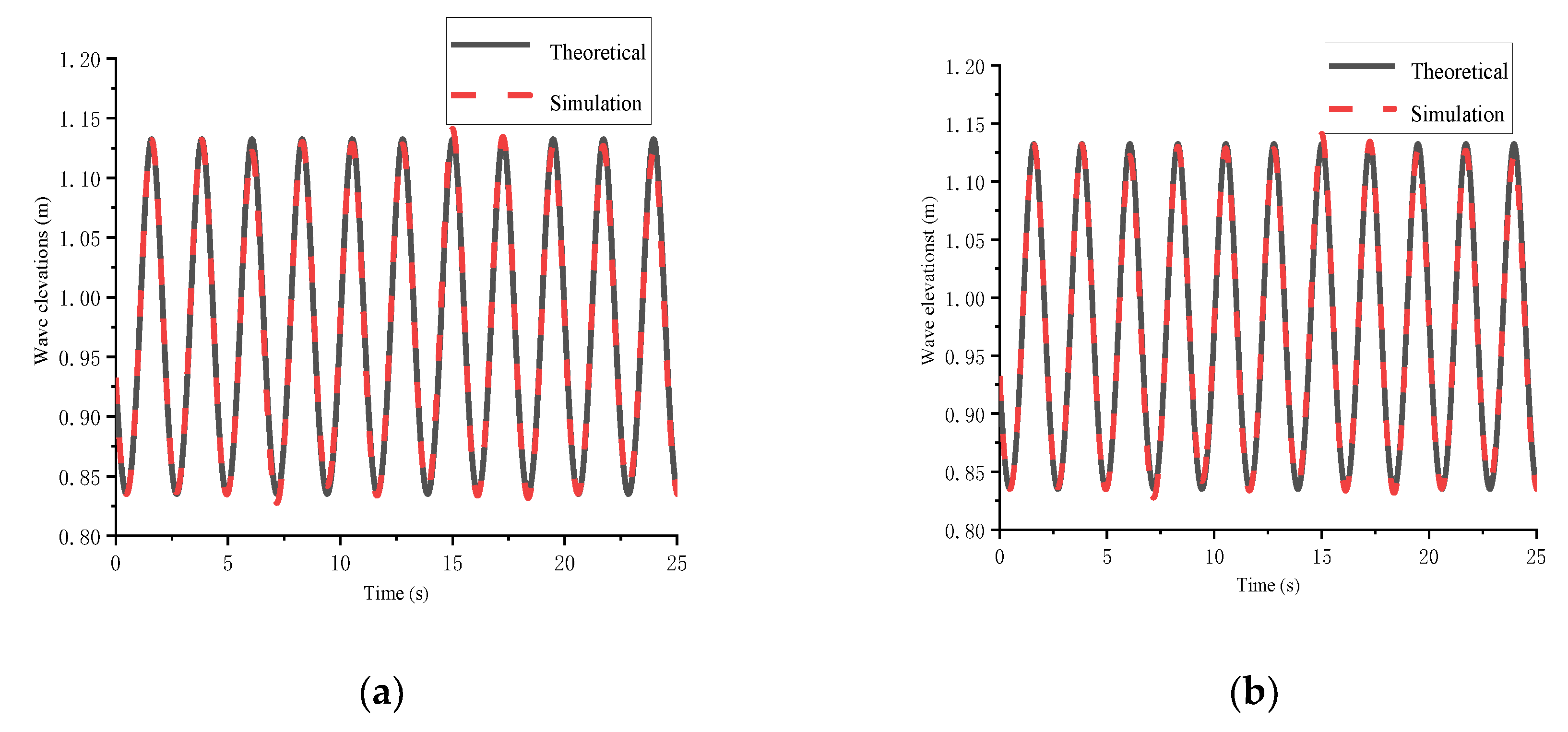
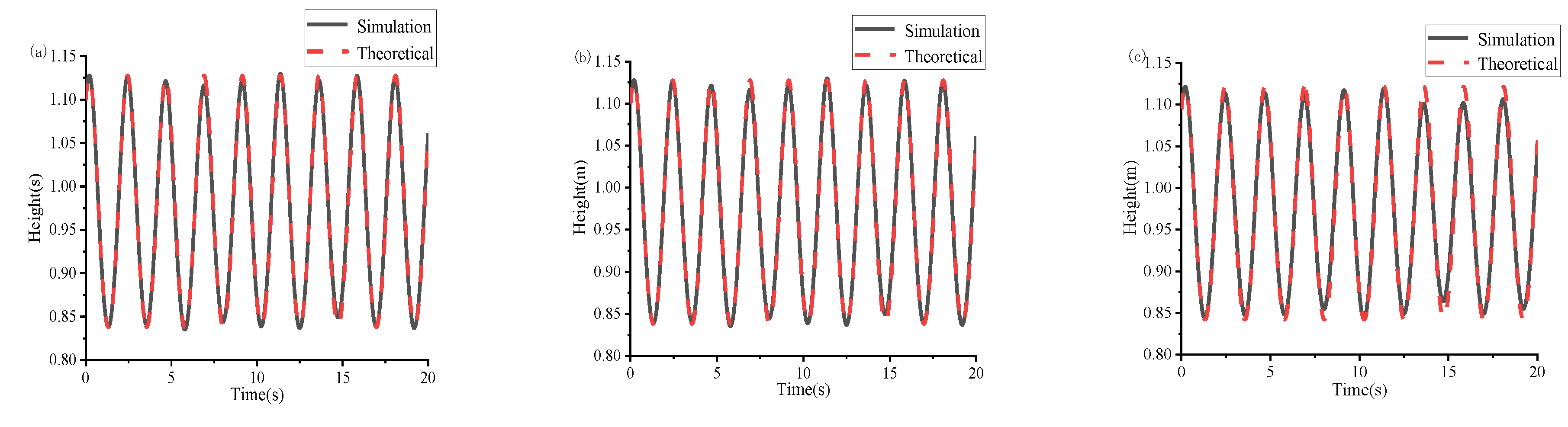
3.4.2. Simulation and Theoretical Comparison of Numerical Wave Generation

In the CFD software STARCCM+ used in this study, the monitoring points are set in the numerical wave tank to obtain the wave elevation time series. Two monitoring points are placed at the inlet (4 m) and middle (12 m) to track wave elevations, and the numerical results are compared with the analytical ones, as seen in Figure 5, where good agreements between them can be found, which shows the accuracy of the numerical wave tank in simulating the fifth-order regular wave.

3.4.3. Verification of Convergence of Numerical Tank Grid

The change of mesh size has a significant influence on the attenuation of waves. Among them, the foundation size has the greatest influence on the accuracy of wave simulation. In the numerical simulation, the mesh size of the overlapping area is closely associated with the foundation size. The arrangement of the wave gauge in the numerical wave tank is shown in Figure 6. It is used to calculate the influence of the following different mesh sizes on the results.
In this study, a typical case (T = 10 s and H = 6 m) is chosen to verify the grid setup of the numerical simulation. As shown in Figure 7, for the wave parameters after reduced transformation in the numerical simulation process (T ≈ 2.23 s, H = 0.3 m), the transformation ratio according to the Froude similarity is shown; in Table 5, α represents the scale ratio, and density correction factor γ is 1.025 (ρseawaterfreshwater). Generally, the base size of the grid should be set to 1/50–1/100 of the wavelength (λ) in the numerical wave simulations. The calculated wavelength is obtained as 156 m according to the wavelength λ (=1.56 T2). Three foundation sizes—1 m, 2 m, and 3 m—are discussed to study the influence of mesh size on generated waves. As shown in Figure 7a,b, good agreement between the numerical solutions and theoretical ones for various mesh size values over the overall tested region can be found. With the increase of the foundation sizes, a sizeable discrepancy between the numerical and theoretical results can be found. As shown in Figure 7c, there is apparent wave attenuation after the calculation time exceeds 15 s. By considering the accuracy of wave simulation and wave attenuation, a more stable mesh size setting with a foundation size of 1 m is used.

3.4.4. Computational Domain and Grid Generation

Considering the flow field integrity and grid number limitation in the CFD software STARCCM+, selecting the computational domain is crucial. In this study, a rectangular parallelepiped calculation domain of 39.75 m × 22.00 m × 12.00 m is adopted. As shown in Figure 8, the free liquid surface acted as the dividing line in the numerical wave tank with gas on the top and liquid on the bottom. The distances of the entrance and exit of the calculation domain to the center of mass of the platform are 13.1 m and 26.5 m, respectively. A wave-eliminating region is defined to reduce the damping layer set by the reflection after the wave was transmitted to the pressure boundary. The mooring system consists of eight high-density polyethylene taut moorings, and they are symmetrically arranged. The cable outlet angle is 30 degrees. The anchor radius is 200 m. All eight mooring lines are 226 m long, and they are in tension and maintain a certain pretension. The specific parameters of mooring lines are shown in Table 6.
The overlapping grid technology in CFD software STARCCM+ is used to mesh the semi-submersible platform. The free surface part adopts the prismatic grid, and the cut volume grid is used for the rest part. The mesh sizes of focus areas, including free surface, strut, and buoyancy tank surface, are refined. The wave encryption grid and the overlapping area grid are shown in Figure 9. Since the exit of the computational domain is the dissipation region, the grid of the water surface in the dissipation region is not encrypted to minimize the number of grids and reduce the workload.
To accurately capture the nonlinear characteristics of shallow-water waves and verify the accuracy of the numerical tank, the incident wave model is defined as fifth-order Stokes regular wave. The realization of fifth-order Stokes regular wave in numerical tank also laid a foundation for the subsequent simulation of freak wave. The draft is 15.5 m, and the flow rate is 1.07 m/s, the wave height is 15.8 m, and the period is 9.39 s (in full scale).

3.4.5. Attenuation Test with Experimental Results

Errors in the model structure, slight wave attenuation, and human operations will bias the results. The decay tests are repeated five times, and average values of these results are determined as the final results to ensure the accuracy. The numerical and experimental results of the natural periods of the platform are shown in Table 7. Figure 10 shows the decay curves in different degree of freedoms.
The difference between the numerical simulation period of heave, roll, and pitch, and the model period, is 2.96%, 0.6%, and −0.33%, respectively. The results are relatively close and are controlled by 5%, which verifies the accuracy of the grid size and calculation method in the numerical simulation.

3.5. Analysis of Slamming Pressure

To verify the accuracy of the finite element model in the CFD method and the feasibility of the analysis method, two cases of typical working conditions are studied in model tests. The measured and simulated slamming pressure time series are compared. The occurrence time, peak value, and error range of slamming are discussed.
The head sea wave condition with H(wave height) of 20 m, T(wave period) of 11 s is studied, which corresponds to H of 0.2 m, T of 1.1 s in model tests. The numerical and experimental wave-slamming time series at the K-point (the K-point at the midline of the vertical surface of the column, as shown in Figure 3) are compared in Figure 11, where three stable periods are used for the analysis. In Figure 11, it can be found that:
(1)
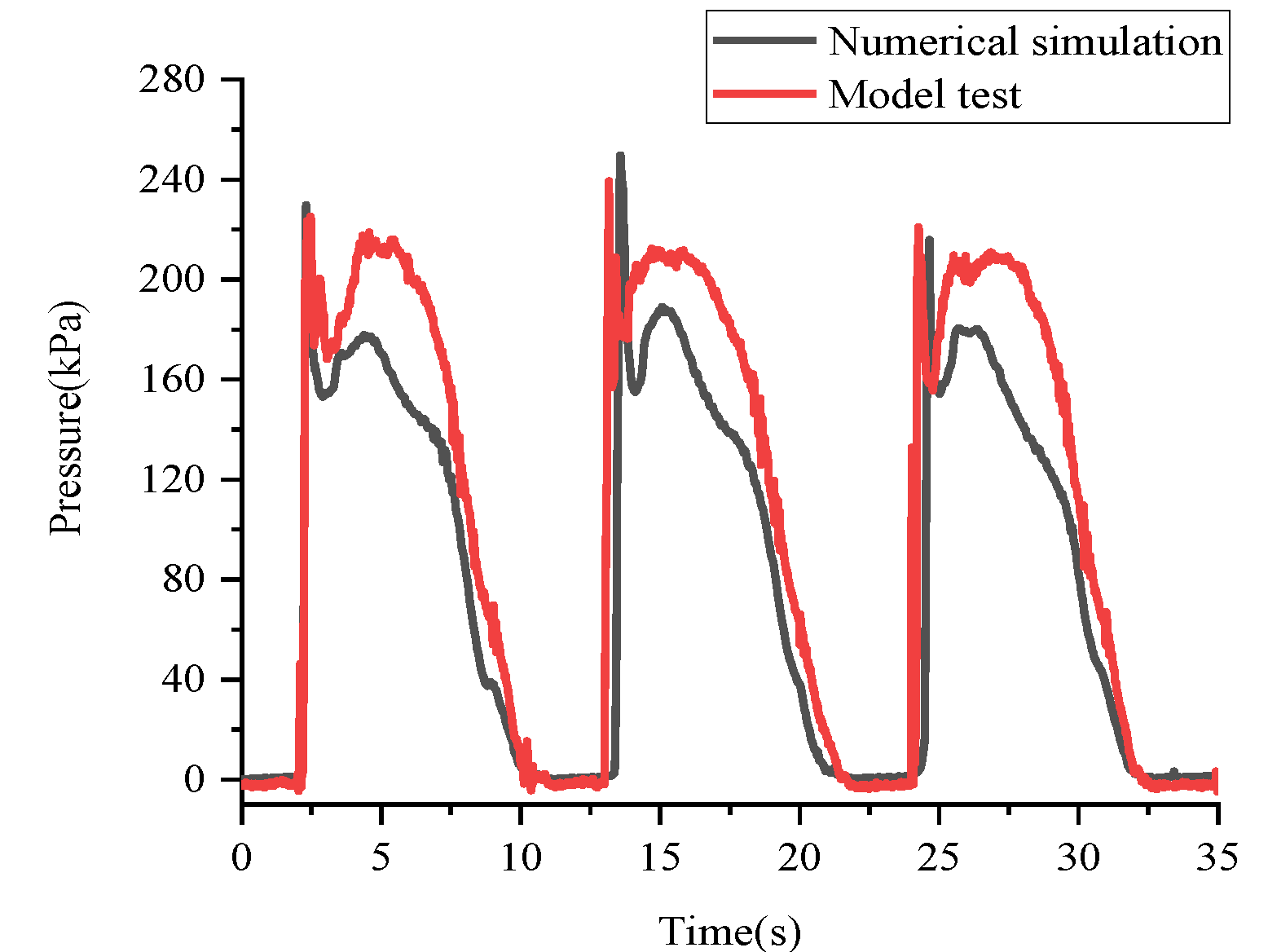
Both the numerical and test results show that the slamming period is about 11 s, which indicates that the numerical simulations are accurate enough and experimental tests are well conducted;
(2)
The simulated slamming pressure time series have the same trend as the experimental ones. The results show similar characteristics: short duration and significant nonlinearity;
(3)
The peak values of numerical slamming pressures are 230.9 kPa, 250.18 kPa, and 223.04 kPa, respectively, in these three wave periods, and the measured slamming peaks are 227.76 kPa, 240.54 kPa, and 218.13 kPa. The differences between them are 1.4%, 3.9%, and 2.3%, respectively. The results are close and within the allowable error range.
The heave sea wave condition with H (wave height) of 15 m, T (wave period) of 9 s is studied, which corresponds to H of 0.15 m, T of 0.9 s in model tests. The results at the K-point are compared in Figure 12. Again, three stable periods were chosen for the analysis, and the findings are concluded as followings:
(1)
Both the numerical results and the test results show that the period is about 9 s;
(2)
The development of slamming pressure at K-point is as follows: firstly, the slamming pressure increases sharply and steeply to the maximum, then decreases rapidly in 0.2–0.3 s, and decreases slowly till to the end. If compared with Figure 11, it can be found that the nonlinearity of the slamming pressure is more evident in this case. However, the fluctuating water pressure is less prominent than the one in the first case;
(3)
The simulated peaks of slamming pressures are 220.50 kPa, 213.85 kPa, and 210.09 kPa, respectively, and the measured ones are 245.52 kPa, 231.74 kPa, and 232.47 kPa. The differences between them are −10.2%, −7.7%, and −9.6%, respectively. The results are close and within the allowable error range.

4. Study on Load Distribution of Platform under Freak Wave in Numerical Simulation

4.1. Load Characteristics of Slamming Pressure

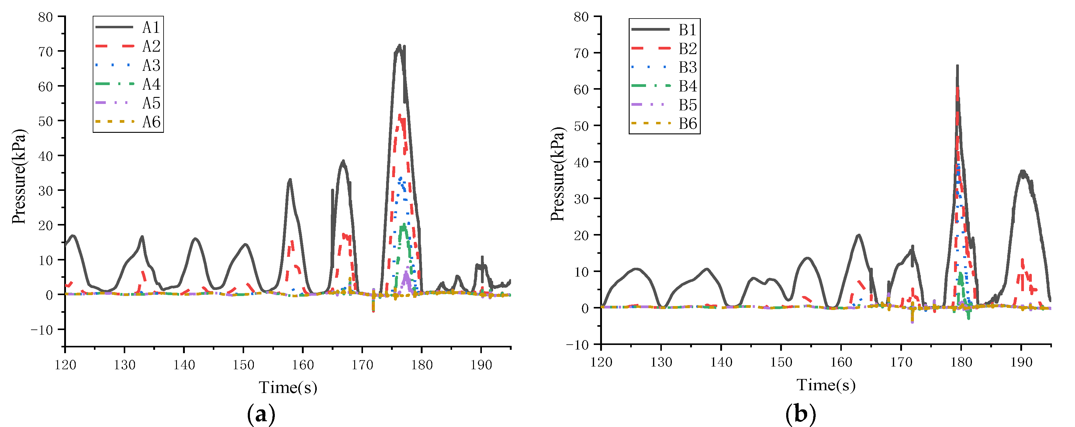
4.1.1. Slamming Loads in Head Sea

In Section 3, it has been validated that the numerical software is able to present good estimations of the slamming load. In the following study, the numerical simulations are carried out to study slamming load due to snap loads.
Figure 13 shows the slamming pressure time series of L1 to L8 when the draft is 15.5 m and the flow rate is 1.07 m/s. Under the random wave condition between 100 and 150 s, it can be found that the maximum slamming pressure is only 35.39 kPa (hereafter, this value is denoted as a normal slamming value). After 158 s, the slamming value increases rapidly, which is as great as 60.76 kPa and 78.92 kPa at 158.7 s and 165.73 s, respectively, and they are 71.69% and 123% higher than the normal slamming value. The maximum slamming appears at the L1 in 175 s due to the freak wave, and the ultimate value is 137.2 kPa, which is 287.68% greater than the normal slamming value. It is 73.8% and 96% greater than the two neighbor slamming values, respectively. L1–L8 are located at a quarter of the front surface of the column, and the height increases in turn, while the slamming value and the area formed by the negative air gap are decreased successively. This indicates that the area when the L1 is located should be strengthened to resist vast slamming loads under freak waves.
As shown in Figure 13b, during the period from 165 to 180 s, there are two slamming waves in a single wave period. That is because the wave’s massive stacking and height increase in front of the platform when the freak wave impacts the platform for the first time. Additionally, the platform moves more violently under the influence of the freak wave, which leads to the platform slamming for the second time. In this slamming process, the water pressure occupies the main component, mainly manifested by the slow decay process of the slamming pressure. The effect of the freak wave will cause a sudden change and rapid increase of the slamming value, and the damage to the platform cannot be ignored.
Figure 14 and Figure 15 show the slamming pressure time histories of D and LZ. It is seen that the slamming occurs at D2 and D3, and LZ2, LZ3, and LZ4, points. The maximum pressures of D2 and D3 are 15.13 kPa and 44.4 kPa. The maximum values of LZ2 and LZ3 are 33.3 kPa and 85.3 kPa. The slamming pressures of LZ2 and LZ3 are 220% and 192% of D2 and D3, respectively, which indicates that the slamming loads on the rear column are much larger than the front column. The negative air gap appears around the column due to the run up of wave.
Negative pressures can be found in Figure 14b and Figure 15b, where it is seen that these negative pressures last for around 1 s when the slamming pressure is reduced to 0 kPa. The occurrence of negative pressures means that waves subside rapidly after the impact, and there is no air to supplement in time. Freak waves run up at the junction of the bottom of the deck and the column. Due to the fact that the two vertical plates are connected at 90°, the waves are squeezed and collided here, showing strong nonlinear characteristics.

4.1.2. Slamming Loads in Beam Sea

The slamming load on offshore structure in beam sea is rare; however, it should be discussed as an exceptional hazardous working condition. Figure 16a shows the wave slamming on the monitoring points arranged on the front column wavefront surface (A1–A6), and Figure 16b shows the wave slamming on the monitoring points located on the rear column wavefront surface (B1–B6). It can be seen that the pressure distribution on the front column wavefront surface is relatively gentle and the pressure distribution on the rear column wavefront surface is relatively steeper. The reason is that when the wave is a transverse wave, the front column wavefront surface is located on the side of the platform, and there is no deck cover at the top. However, there is wave interference on the wave face of the rear column, and there is a shadowing effect between the column and the deck. So, the nonlinear characteristics of wave slamming on the rear column are more prominent.
The maximum slamming value decreases with the increase of vertical height. The maximum values of A1, A2, and A3 are 71.7 kPa, 51.7 kPa, and 33.7 kPa, and the maximum values of B1, B2, and B3 are 66.4 kPa, 61.9 kPa, and 40.11 kPa. It is seen that the slamming value of the rear column is slightly smaller than that of the front column, except for A1.

4.2. Characteristics of Slamming Pressure Distribution

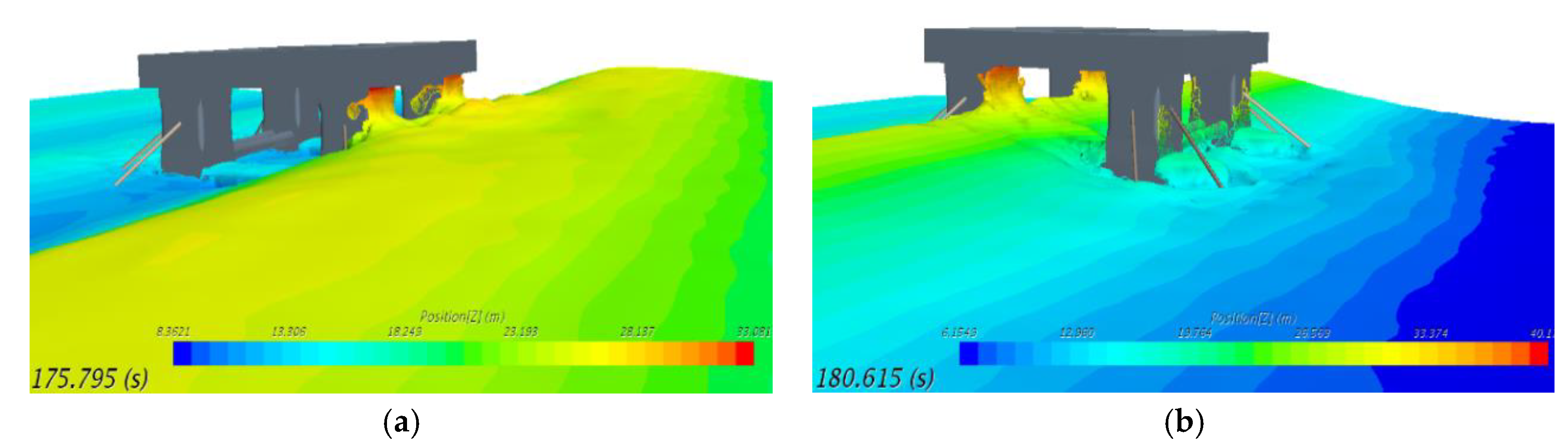
4.2.1. Free Surface Variations

Two instantaneous dates, including 175.795 s and 180.615 s, are selected to analyze the variations of the free water surface, and the results are shown in Figure 17. At 175.795 s, the wave collided with the deck on the wavefront surface of the front column, and the run up of wave occurred. When it rises to the top of the column, it squeezes against the bottom of deck box, and the wave shows unique characteristics such as rolling and breaking. At 180.615 s, the wave propagates to the wavefront surface of the rear column. There is also a run up of wave and the wave slamming with the bottom deck, resulting in negative air gap. The variations of free surface can be verified by deck slamming pressure distribution (in the next sub-section).

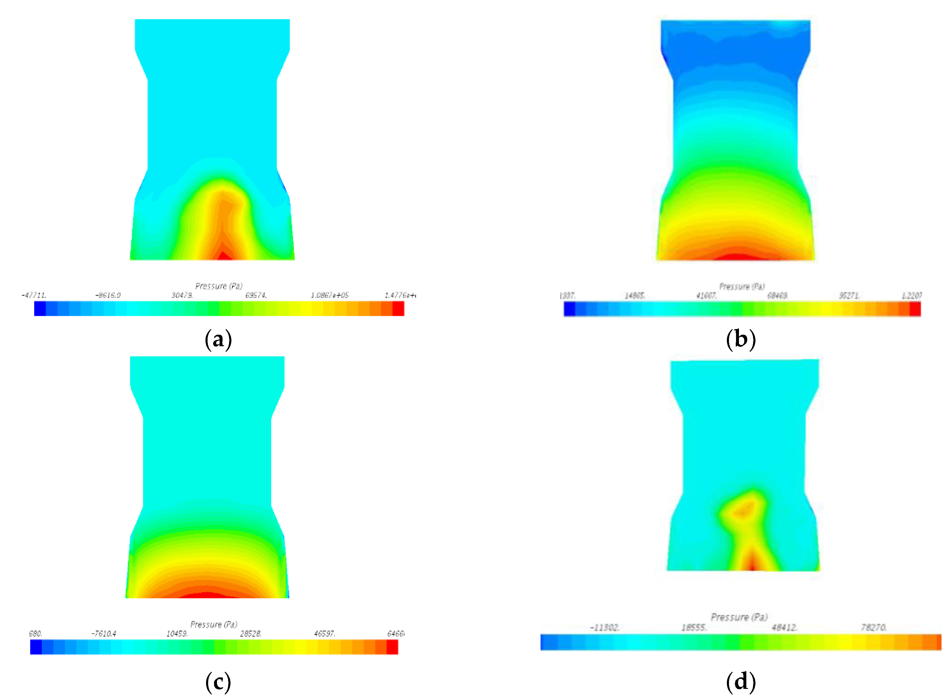
4.2.2. Column Pressure Distribution

The pressure distribution nephograms of wave slamming between 175.795 s and 184.08 s in beam sea are selected to analyze the pressure distribution characteristics of wave slamming on column.
As shown in Figure 18, it can be concluded that the pressure distribution is concentrated in the middle of the column bottom at t1. This indicates that the waves are more clearly superimposed in the center. At t2, the pressure distribution gradually decreases with height rise, resulting in the run up of wave. At this time, the higher position of the column is submerged, and pressure is also generated at the top of the column. At t3 and t4, the wave gradually reduces, which gives rise to a lower pressure area. Moreover, a relatively obvious pressure area is formed on the surface of the column, there is wave slamming on the surface of the column break and separately on the surface, and the area of the high-pressure area is then expanded to two. It can be understood that wave slamming occurs at the junction of the bottom of the column and the buoyancy tank. With the slimness of each periodic wave, a large local slamming pressure is generated.
Due to the run up of the wave, the high-stress area moves up at t2, and the high-stress area at other times is concentrated below the column. The results show that the position below the midpoint of column height is easy to subject wave slamming. The air gap response in this area should be emphatically analyzed during the platform design.

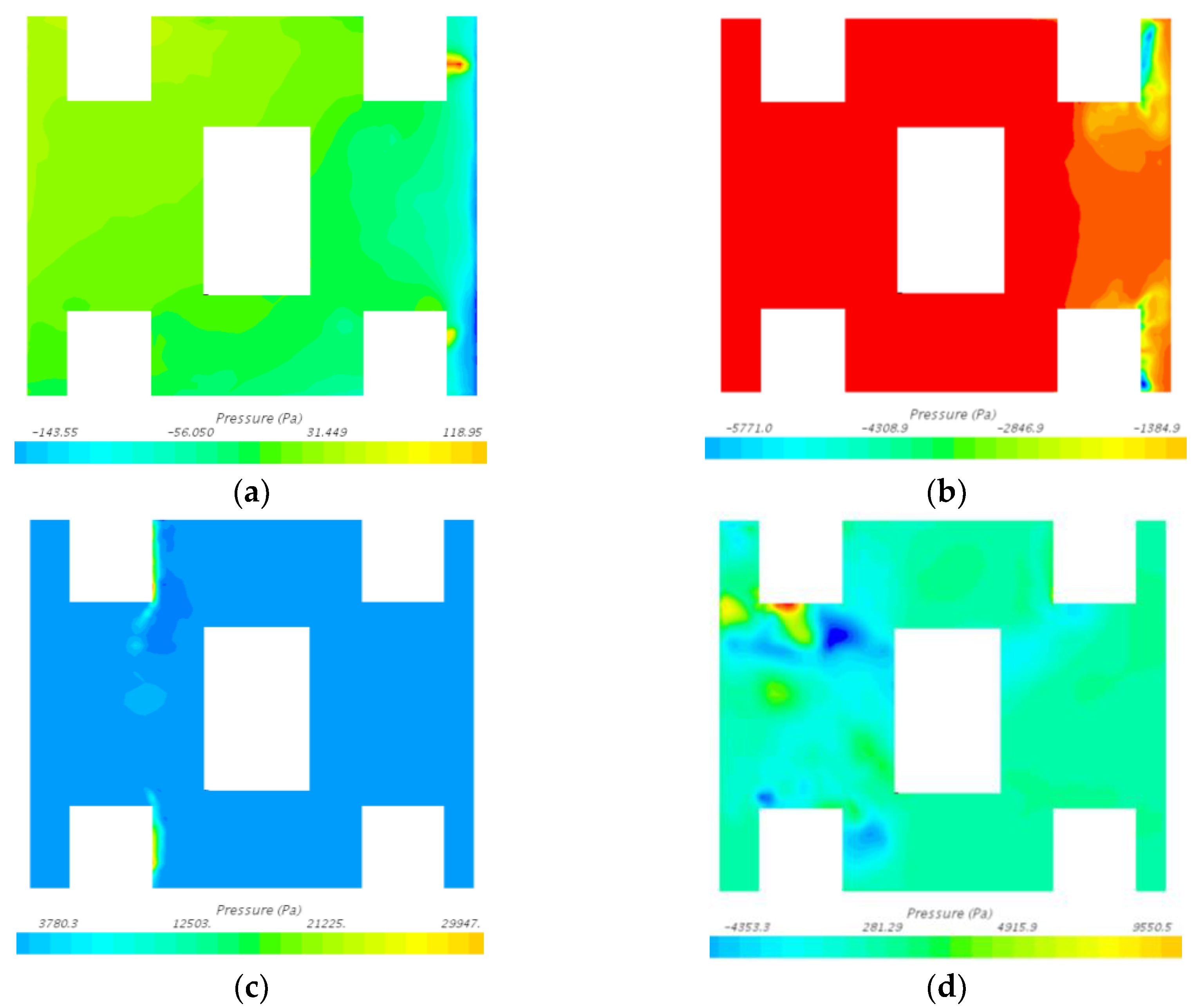
4.2.3. Deck Pressure Distribution

The pressure distribution nephograms of wave slamming between 175.795 s and 184.08 s in beam sea are studied, and the results are given in Figure 19, where it can be seen that the slamming pressure first appears at the junction of the front column wave face and the deck at t1. At the t2 moment, with the falling off of water particles, negative pressure is generated here. When the wave propagates at the junction of wavefront surface of rear column and the deck, two large slamming pressure regions, which are symmetrical about the y-axis, are generated at t3. Finally, there is a large pressure area that diffuses to the side of the column at t4. These areas are the intense slamming of the deck jet generated at t3.
The slamming area from t1 to t4 is generally concentrated at the junction of the column and the deck, which indicates that the column is also an important concern of the air gap response when analyzing the pressure distribution of the deck.

5. Conclusions

In this study, the air gap motion response and wave slamming characteristics of offshore platform under freak wave are numerically and experimentally studied. The difference between experimental and the numerical natural periods of the platform is less than 5%. In the analysis of slamming pressure, the error ranges of slamming pressure under H (wave height) of 20 m, T (wave period) of 11 s are 1.4%, 3.9%, and 2.3%, respectively. The error ranges of slamming pressure under H (wave height) of 15 m, T (wave period) of 9 s are −10.2%, −7.7% and −9.6%, respectively. These results verified the accuracy of the finite element model.
The area of negative air gap and slamming pressure distribution characteristics of the platform under freak wave are studied, and the following conclusions can be drawn:
(1)
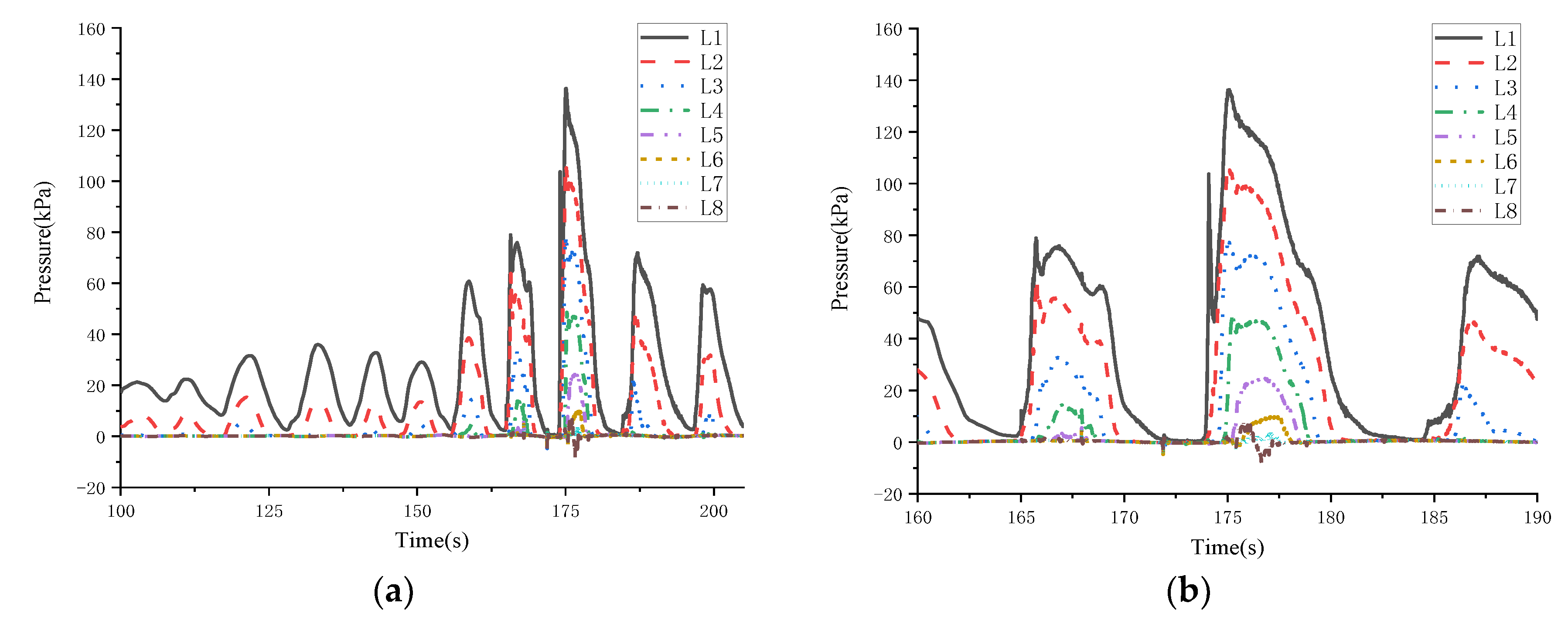
A large slamming with a value of 137.2 kPa occurs under the column near the strut, which is 287.68% greater than the normal slamming value and 73.8% and 96% greater than the two neighbor slamming values. It shows that the freak wave has strong nonlinear characteristics;
(2)
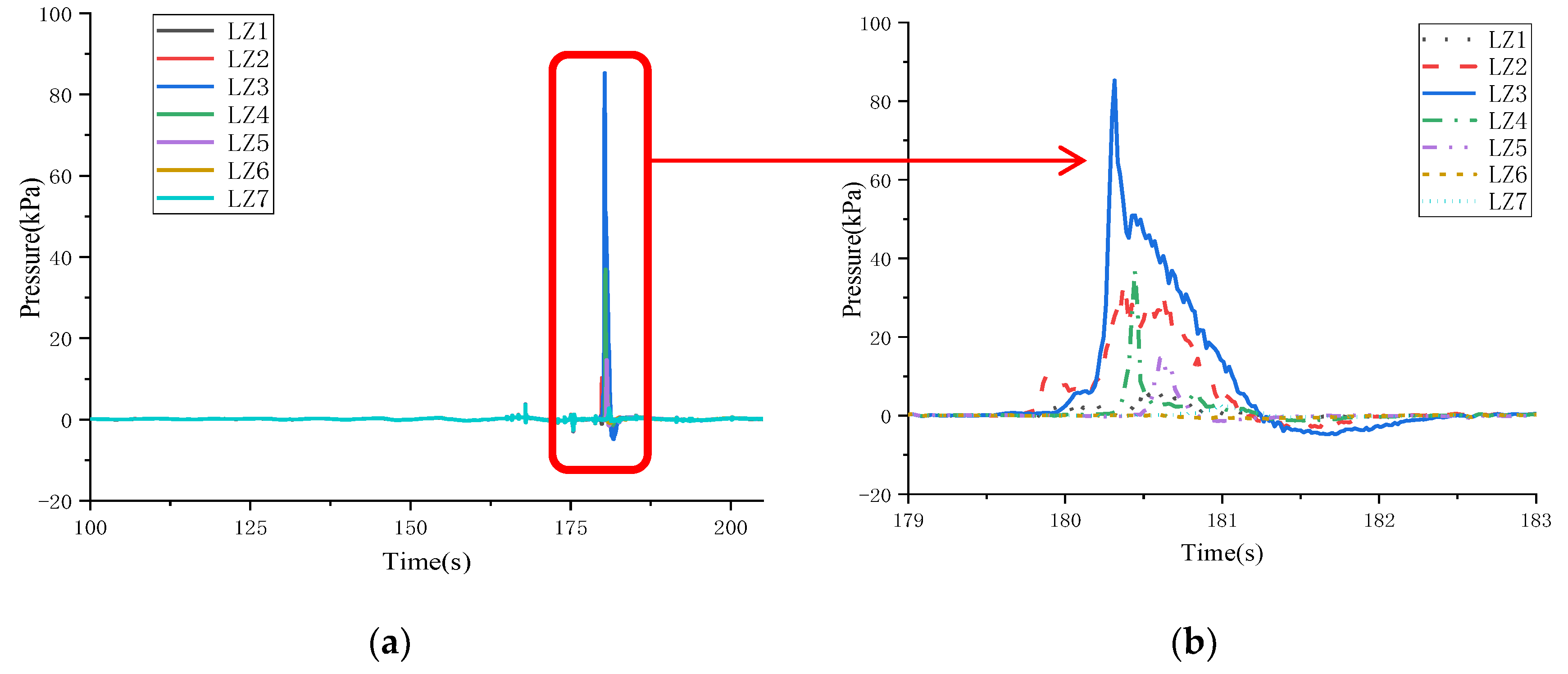
A negative air gap phenomenon is found at five points when analyzing the monitoring points at the bottom of deck box. The slamming pressures of the rear column (LZ2 and LZ3) are 220% and 192% of the front column (D2 and D3), respectively. This shows that the slamming of the deck on the wave face of the rear column is much larger than that on the wave face of the front column. The negative air gap appears around the column due to the wave run-up;
(3)
The slamming values at the same position on the wavefront side of the front column are 7.4%, −19.7%, and −19%, compared with that on the wavefront side of the rear column in beam sea. The results indicate that the nonlinear characteristics of the wavefront side of the rear column are more apparent, and the influence of the freak wave on the rear column is more incredible;
(4)
It is found that the part below the midpoint of the column height is easy to subject to larger slamming than other positions, and the high-stress area of slamming is generally concentrated at the junction of column and deck.
The analysis shows that the freak wave has strong nonlinear characteristics. The influence of the maximum peak energy on the platform cannot be ignored. Especially when the freak wave appears, the slamming pressure is two to three times higher than usual under the same significant wave height. The negative air gap is closely related to the wave run up of column, which mainly occurs at the junction of the column and the buoyancy tank. This result provides a reference for the structural areas that need to be strengthened in the design of the semi-submersible platform. In addition, the wave slamming load has a greater impact on the strength of slender pole structures such as struts. Finally, the research on the formation mechanism of freak waves, the conditions and rules of occurrence, and the movement characteristics of platform operations under freak wave are very important to the design and operational safety of platforms.

Author Contributions

Conceptualization, F.H. and H.Y.; methodology, F.H., H.Y. and S.X.; software, H.Y., Z.Y. and K.A.; validation, F.H., H.Y. and S.X.; formal analysis, H.Y., Z.Y. and K.A.; investigation, F.H.; resources, F.H.; data curation, H.Y.; writing—original draft preparation, F.H., H.Y. and S.X.; writing—review and editing, F.H. and S.X.; visualization, H.Y.; supervision, F.H. and S.X.; project administration, F.H.; funding acquisition, F.H. All authors have read and agreed to the published version of the manuscript.

Funding

This research was funded by the National Natural Science Foundation of China, grant number 52071161.

Institutional Review Board Statement

Not applicable.

Informed Consent Statement

Not applicable.

Data Availability Statement

Not applicable.

Acknowledgments

This work was financially supported by the National Natural Science Foundation of China (Grant No. 52071161). The support is gratefully acknowledged by the authors.

Conflicts of Interest

The authors declare no conflict of interest.

References

  1. Russell, R.C.H.; Macmillian, D.H. Waves as Tides; Greenwood Press: Westport, CY, USA, 1970. [Google Scholar]
  2. Baarholm, R.; Faltinsen, O.M. Wave impact underneath horizontal decks. J. Mar. Sci. Technol. 2004, 9, 1–13. [Google Scholar] [CrossRef]
  3. Jiang, C.X.; Wang, H.; Hu, J.J.; Xu, C. Wave load model test investigation of deep sea semi-submersible platform. Ship Sci. Technol. 2017, 39, 100–104. [Google Scholar]
  4. Zhang, S.G.; Dick, K.P.Y.; Katsuji, T. Simulation of plunging wave impact on a vertical wall. J. Fluid Mech. 1996, 327, 221–254. [Google Scholar] [CrossRef]
  5. Faltinsen, O.M. Wave loads on offshore structures. Annu. Rev. Fluid Mech. 1990, 22, 35–56. [Google Scholar] [CrossRef]
  6. Jain, A.K. Nonlinear coupled response of offshore tension leg platforms to regular wave forces. Ocean. Eng. 1997, 24, 577–592. [Google Scholar] [CrossRef]
  7. Nielsen, F.G. Comparative study on air-gap under floating platforms and run-up along platform columns. Mar. Struct. 2003, 16, 97–134. [Google Scholar] [CrossRef]
  8. Liu, J.C.; Guo, Y.H.; Xiao, L.F.; Teng, X.Q.; Wang, J.G.; Xu, L.X.; Lu, H.D. An experimental study of wave impact loads on a drilling semi-submersible platform. Offshore Eng. Equip. Technol. 2018, 5, 234–237. [Google Scholar]
  9. Huo, F.L. Influence of water depth on hydrodynamic performance and wave load of semi-submersible platform. Ship Eng. 2014, 36, 100–104. [Google Scholar]
  10. Simos, A.N.; Sparano, J.V.; Aranha, J.A.P.; Matos, V.C.L. Second-order hydrodynamic effects on resonant heave, pitch and roll motions of a large-volume semi-submersible platform. In Proceedings of the 27th International Conference on Offshore Mechanics and Artic Engineering, Estoril, Portugal, 15–20 June 2008. [Google Scholar]
  11. Lwanowski, B.; Marc, L.; Wemmenhove, R. CFD simulation of wave run-up on a semi-submersible and comparison with experiment. In Proceedings of the ASME 2009 28th International Conference on Ocean, Offshore and Arctic Engineering, Honolulu, HI, USA, 31 May–5 June 2009. [Google Scholar]
  12. Li, J.; Huang, Z.; Tan, S.K. Extreme air-gap response below deck of floating structures. Int. J. Ocean Clim. Syst. 2010, 1, 15–26. [Google Scholar] [CrossRef]
  13. Jiang, Y.C.; Li, M.; Yang, S.G. A new method to simulate freak wave with fewer cosine waves. China Offshore Oil Gas 2009, 21, 138–144. [Google Scholar]
  14. Deng, Y.F.; Tian, X.L.; Li, X. Study on nonlinear characteristics of freak-wave Forces with different wave steepness. China Ocean. Eng. 2019, 33, 608–617. [Google Scholar] [CrossRef]
  15. Dyachenko, A.I.; Kachulin, D.I.; Zakharov, V.E. Probability distribution functions of freak waves: Nonlinear versus linear model. Stud. Appl. Math. 2016, 137, 189–198. [Google Scholar] [CrossRef]
  16. Zhang, Y.Q.; Hu, J.P.; Sheng, S.W.; Ye, Y.; You, Y.G.; Wu, B.J. Rapid Simulation of freak wave generation based on a nonlinear model. Recent Progresses in Fluid Dynamics Research. In Proceedings of the Sixth International Conference on Fluid Mechanics, Guangzhou, China, 30 June–3 July 2011. [Google Scholar]
  17. Gao, N.B.; Yang, J.M.; Zhao, W.H.; Li, X. Numerical simulation of deterministic freak wave sequences and wave-structure interaction. Ships Offshore Struct. 2016, 11, 802–817. [Google Scholar] [CrossRef] [Green Version]
  18. Huang, Y.L.; Hu, J.P.; Liu, S.H. Numerical simulation of oceanic freak waves based on FLUENT. Guangdong Shipbuild. 2017, 36, 17–20. [Google Scholar]
  19. Zhang, X.Y.; Hu, Z. Dynamic response of vertical plates under green water impact induced by freak waves. J. Harbin Eng. Univ. 2018, 39, 268–273. [Google Scholar]
  20. Zhang, W.X.; Lu, C. Analysis of response of semi-submersible platform under freak wave. Shipbuild. Technol. 2016, 5, 35–41. [Google Scholar]
  21. Wei, Y.F.; Liu, Z.; Xia, Z.D.; Wang, Z.N.; Wang, D.J. Model test study of wave load on a tumblehome ship in freak waves. China Shipbuild. 2020, 61, 11–19. [Google Scholar]
  22. Peregrine, D.H. Water-wave impact on wall. Annu. Rev. Fluid Mech. 2003, 35, 23–43. [Google Scholar] [CrossRef]
  23. Clauss, F.; Schmittner, C.; Hennig, J. Simulation of rogue waves and their impact on marine structures. In Proceedings of the MAXWAVE Final Meeting, Geneva, Switzerland, 8–10 October 2003. [Google Scholar]
  24. Dong, G.H.; Gao, X.; Mao, X.Z.; Ma, Y. Energy properties of regular water waves over horizontal bottom with increasing nonlinearity. Ocean Eng. 2020, 218, 108159. [Google Scholar] [CrossRef]
Figure 1. A superposition of 20 cosine waves. (a) Time history of wave elevations by numerical simulation. (b) Freak wave profile.
Jmse 09 01266 g001
Figure 2. Semi-submersible platform. (a) Numerical platform configuration. (b) Test platform model.
Jmse 09 01266 g002
Figure 3. Distribution of the monitoring points. (a) Column monitoring points. (b) The bottom of deck box monitoring points.
Jmse 09 01266 g003
Figure 4. Wave elimination region.
Jmse 09 01266 g004
Figure 5. Comparison between theoretical numerical and waveform. (a) 4 m from the calculation domain entrance. (b) 12 m from the calculation domain entrance.
Jmse 09 01266 g005
Figure 6. Installation position of wave gauge.
Jmse 09 01266 g006
Figure 7. Wave time history of three foundation sizes. (a) Foundation size: 1 m. (b) Foundation size: 2 m. (c) Foundation size: 3 m.
Jmse 09 01266 g007
Figure 8. Numerical wave tank. (a) Computational domain. (b) Boundary condition.
Jmse 09 01266 g008
Figure 9. Wave encryption grid and overlapping area grid. (a) Wave encryption grid. (b) Overlapping area grid.
Jmse 09 01266 g009
Figure 10. Decay cures in different degrees of freedom. (a) Heave. (b) Roll. (c) Pitch.
Jmse 09 01266 g010
Figure 11. Comparison of K-point slamming pressure under the wave condition with H = 20 m, T = 11 s.
Jmse 09 01266 g011
Figure 12. Comparison of K-point slamming pressure under the wave condition with H = 15 m, T = 9 s.
Jmse 09 01266 g012
Figure 13. Pressure time history curve of L1–L8 monitoring point on front surface of column. (a) Global graphics. (b) Detail graphics.
Jmse 09 01266 g013
Figure 14. Pressure time series of D1–D7 on wavefront surface of front column. (a) Global graphics. (b) Detail graphics.
Jmse 09 01266 g014
Figure 15. Pressure time series of LZ1–LZ7 on wavefront surface of rear column. (a) Global graphics. (b) Detail graphics.
Jmse 09 01266 g015
Figure 16. Pressure time series of column monitoring points. (a) The monitoring points of A1–A6. (b) The monitoring points of B1–B6.
Jmse 09 01266 g016
Figure 17. Evolution of free surface at two moments under freak wave. (a) t = 175.795 s. (b) t = 180.615 s.
Jmse 09 01266 g017
Figure 18. Slamming pressure distribution of column at different time. (a) t1 = 175.795 s. (b) t2 = 176.575 s. (c) t3 = 180.615 s. (d) t4 = 184.08 s.
Jmse 09 01266 g018
Figure 19. Slamming pressure distribution of deck in head sea wave condition. (a) t1 = 175.795 s. (b) t2 = 176.575 s. (c) t3 = 180.615 s. (d) t4 = 184.08 s.
Jmse 09 01266 g019
Table 1. The period and wave height of 20 cosine waves.
CasesT (s)H (m)CasesT (s)H (m)
A128.560.05A1112.080.94
A225.130.30A1211.420.84
A322.440.72A1310.830.76
A420.271.08A1410.300.68
A518.481.29A159.820.61
A616.981.35A169.380.55
A715.711.33A178.980.50
A814.611.25A188.610.45
A913.661.15A198.270.41
A1012.821.04A207.950.38
Table 2. Dimensions of platform body and model.
Structure NameActual SizeNumerical Model SizeTest Model SizeUnit
Buoyancy tank (L × w × h)104.5 × 3.9 × 10.055.225 × 0.195 × 0.51.045 × 0.039 × 0.1005m
Main deck height37.551.87750.3755m
Double bottom height29.551.47750.2955m
Center spacing of buoyancy tanks37.51.8750.375m
Longitudinal column spacing55.02.75150.55m
Working draft/drainage volume15.5/38,4000.775/4.80.155/0.0384m/m³
Table 3. Hydrostatic parameters of full-scale model.
Center of Gravity (m)Center of Buoyancy (m)Radius of Gyration (m)
longitudinal center of gravity
(LCG)
transverse center of gravity
(TCG)
vertical center of gravity
(VCG)
longitudinal center of buoyance
(LCB)
transverse center of buoyance
(TCB)
vertical center of buoyance
(VCB)
RxRyRz
0.050.023.40.10.06.529.931.634.5
Table 4. The coordinates of the monitoring points.
Monitoring PointsX (m)Y (m)Z (m)Monitoring PointsX (m)Y (m)Z (m)
K35.25−2713.55B427.5−19.2521
L135.252412B527.5−19.2524
L235.252414B627.5−19.2527
L335.252416D135.2534.7529.55
L435.252418D235.2528.7529.55
L535.252420D335.2522.7529.55
L635.252422D435.2516.7529.55
L735.252424D535.2510.7529.55
L835.252426D635.254.7529.55
A127.534.7512D735.25029.55
A227.534.7515LZ1−19.7534.7529.55
A327.534.7518LZ2−19.7528.7529.55
A427.534.7521LZ3−19.7522.7529.55
A527.534.7524LZ4−19.7516.7529.55
A627.534.7527LZ5−19.7510.7529.55
B127.5−19.2512LZ6−19.754.7529.55
B227.5−19.2515LZ7−19.75029.55
B327.5−19.2518
Table 5. The transformation ratio according to the Froude similarity.
ParameterLabelConversion Coefficient
LengthLs/Lmα
AreaAs/Amα2
PeriodTs/Tmα1/2
ForceFs/Fmγα3
Table 6. Parameter of mooring line.
TypeDiameter
(mm)
Wet Weight
(kg/m)
Dry Weight
(kg/m)
Axial Rigidity
(N)
Breaking Strength (N)
Entity11470.32.57 × 1087.35 × 106
Table 7. Natural period of platform.
Degrees of FreedomModel Period (s)Numerical Simulation Period (s)Error Percentage
Heave20.320.92.96%
Roll33.633.80.6%
Pitch30.029.9−0.33%
Publisher’s Note: MDPI stays neutral with regard to jurisdictional claims in published maps and institutional affiliations.

