
Path Planning for Underwater Information Gathering Based on Genetic Algorithms and Data Stochastic Models

 , ,
, ,  , , , ,
  , and
, and
Abstract
:1. Introduction
2. Materials and Methods
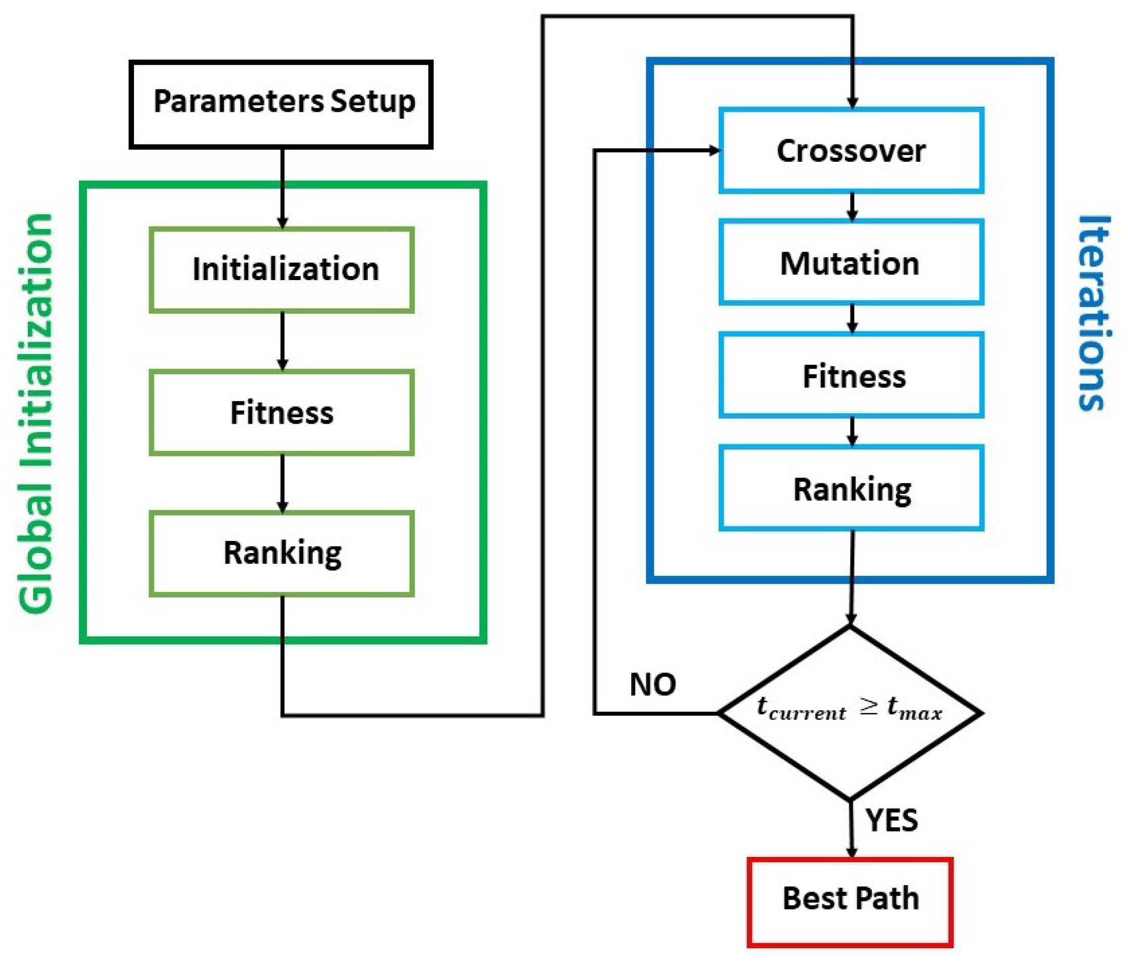
2.1. Genetic Path Planner
- 1.
- The presence of PO is considered time-invariant during all the planning task. The assumption is reasonable as the typical endurance of an AUV is limited to few hours while the variations in PO meadows usually occur over several months.
- 2.
- The boundaries of the area to be explored and the presence of obstacles are considered a priori known. The assumption results appropriate as PO monitoring is carried out periodically in the same geographical areas to assess its spread and health state.
- 3.
- A two-dimensional scenario is considered to represent a path using North and East coordinates referred to the NED frame. The vertical coordinate is beyond the aim of the proposed planner. The considered application of PO monitoring is usually based on optical cameras. The vertical coordinate is thus usually controlled to ensure the AUV to maintain a desired altitude with respect to the sea bottom to guarantee good acquisition conditions.
2.1.1. Consistency Check
2.1.2. Global Initialisation
2.1.3. Crossover
2.1.4. Mutation
2.1.5. Fitness
2.2. Comparative Planners
- (1)
- Sampling-Based planner (S-B)This planner corresponds to the implementation of the planning method proposed in [14], which is considered, to the extent of the authors’ knowledge, as one of the main state-of-the-art IPP approaches for IG operations. The planner is composed of two phases: The first one is called Station Searching and applies a RRT algorithm to find the most informative point within the target area, named as Station. In the second phase, called Informative Path Planner, the planner searches for the optimal path according to a trade-off between the DE of path and its length. With this aim, a RRT* algorithm is utilised to find the best path which connects the start point to the Station, if any, respecting a budget constraint on the travelled distance. In case the RRT* algorithm fails to find a feasible solution, the path obtained during the Station Searching phase is used.
- (2)
- Random PlannerA random planner has been evaluated to assess whether the genetic operations in the iterative part of the GPP algorithm provide an improvement on the performance of the solutions. Otherwise, they would result to be just time consuming operations which can be avoided. Therefore, this planning strategy consists in an extended global initialisation phase, identical to the one implemented in the GPP algorithm, which generates random chromosomes for all the available planning time. Afterwards, using the fitness and ranking operators, the best path among all the generated ones is selected. Although a similar effect on the chromosomes generation could be achieved using high mutation probabilities z and q in the GPP approach, the authors decided to implement the random planner to not perform any kind of optimisation phase in the algorithm. This allows to evaluate the contribution of the optimisation performed by the genetic operations in the GPP algorithm.
2.3. Metrics
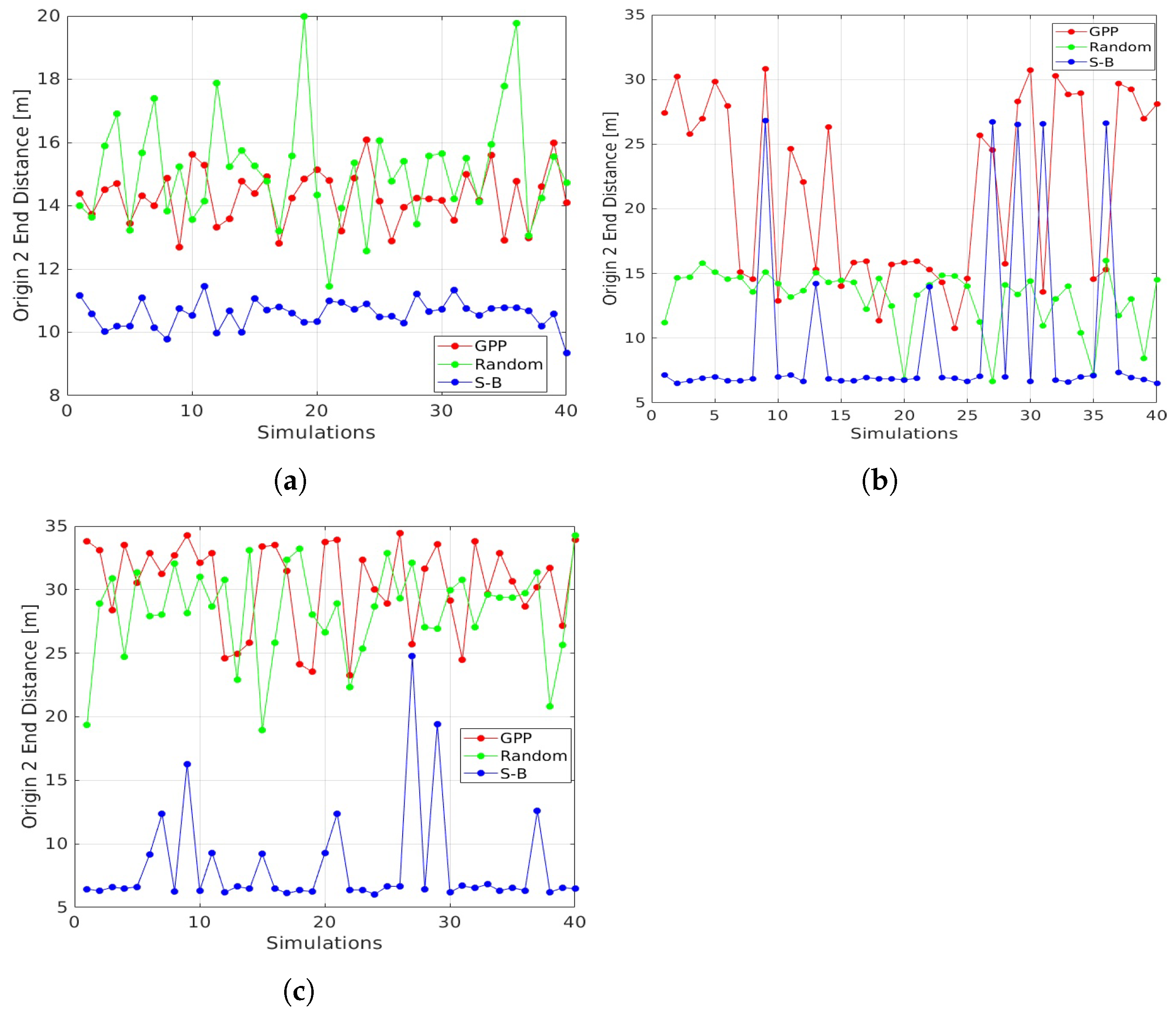
- Distance Origin to End (02E)This metric coincides with the variable adopted as contribution in the GPP utility function, indicated as . It specifies how far the final point is from the starting one, providing a sense of how spread the path is over the target area.
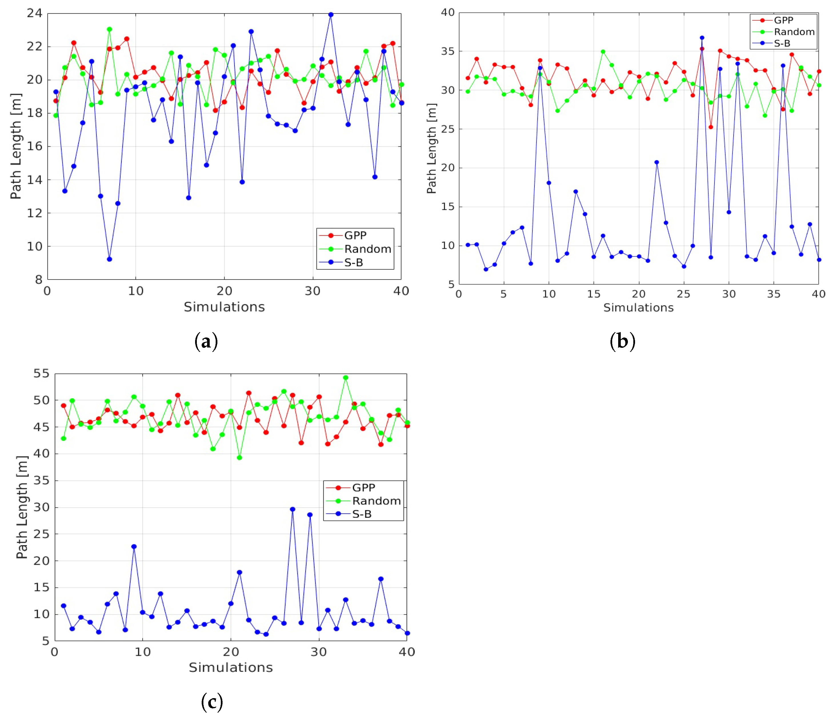
- Path Length (PL)PL is the total length of a path, computed by adding all the distances between consecutive nodes. It is an indicator of how extended the path is, which has to be considered together with the O2E to avoid misleading conclusions. In particular, in those cases where the O2E results to be small, a high value of PL could mean an extended path and, thus, a wider coverage of the area to inspect. On the contrary, for the same O2E value, a small value of PL entails a short path.
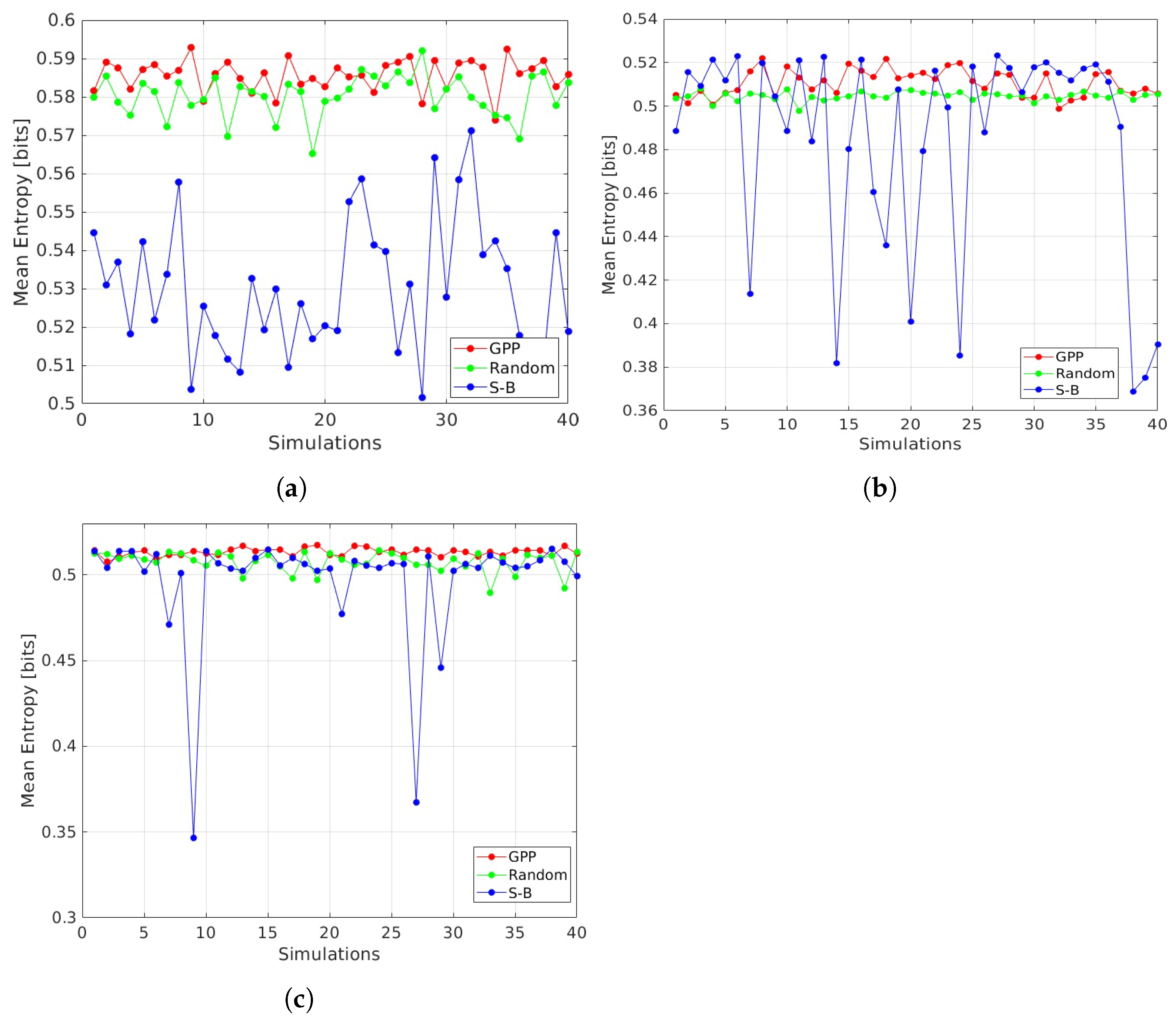
- Mean Entropy (ME)ME calculates the line integral of the DE of the points along the whole path. This is done refining Equation (3) and sampling the path with a resolution r. The ME calculation is defined aswhere P is the evaluated path and represents the path length. In this work, the resolution of the path sampling r is set to 0.2 m. Note that, generally r can differs from , and it is recommendable to always have to increase the accuracy in the computation of the metric ME. Moreover, it is important to highlight that the computation of the metric ME is performed offline. Thus, r can be set according to the desired accuracy of the ME metric without influencing the computational cost of the planners. Therefore, the authors decided to maintain r equal for all the target areas.
3. Results
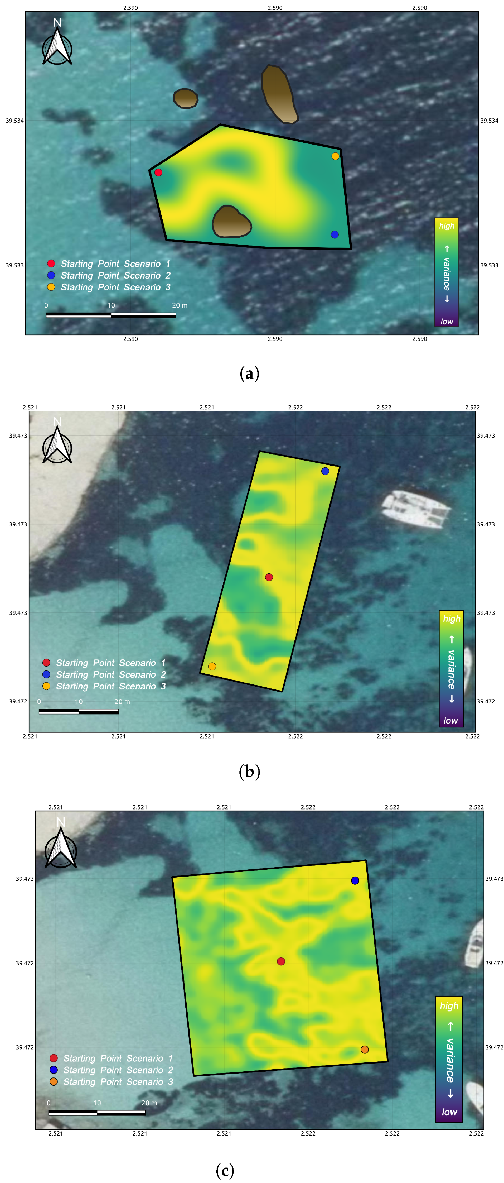
3.1. Test Scenario Description
3.2. GPP Parameter Selection
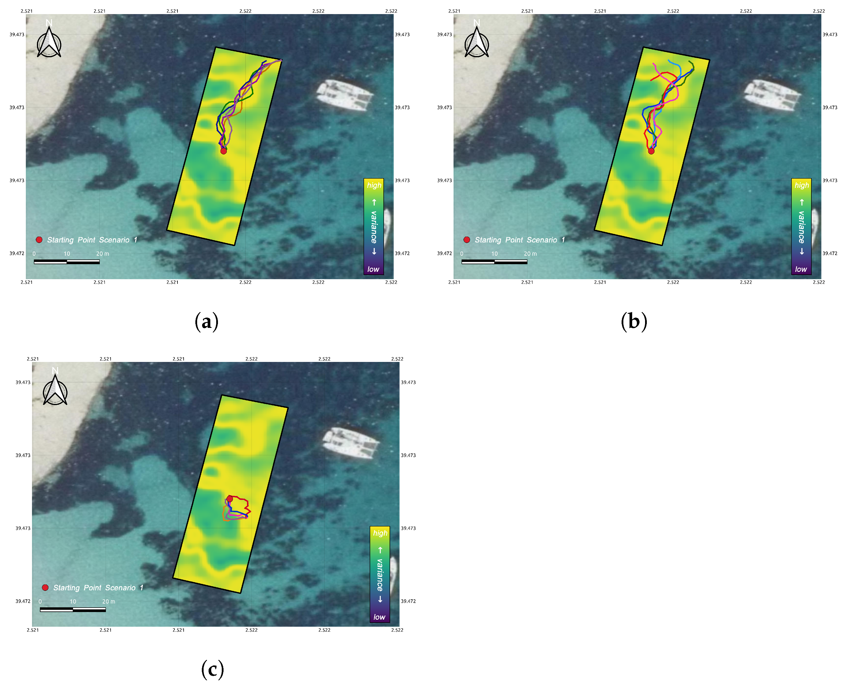
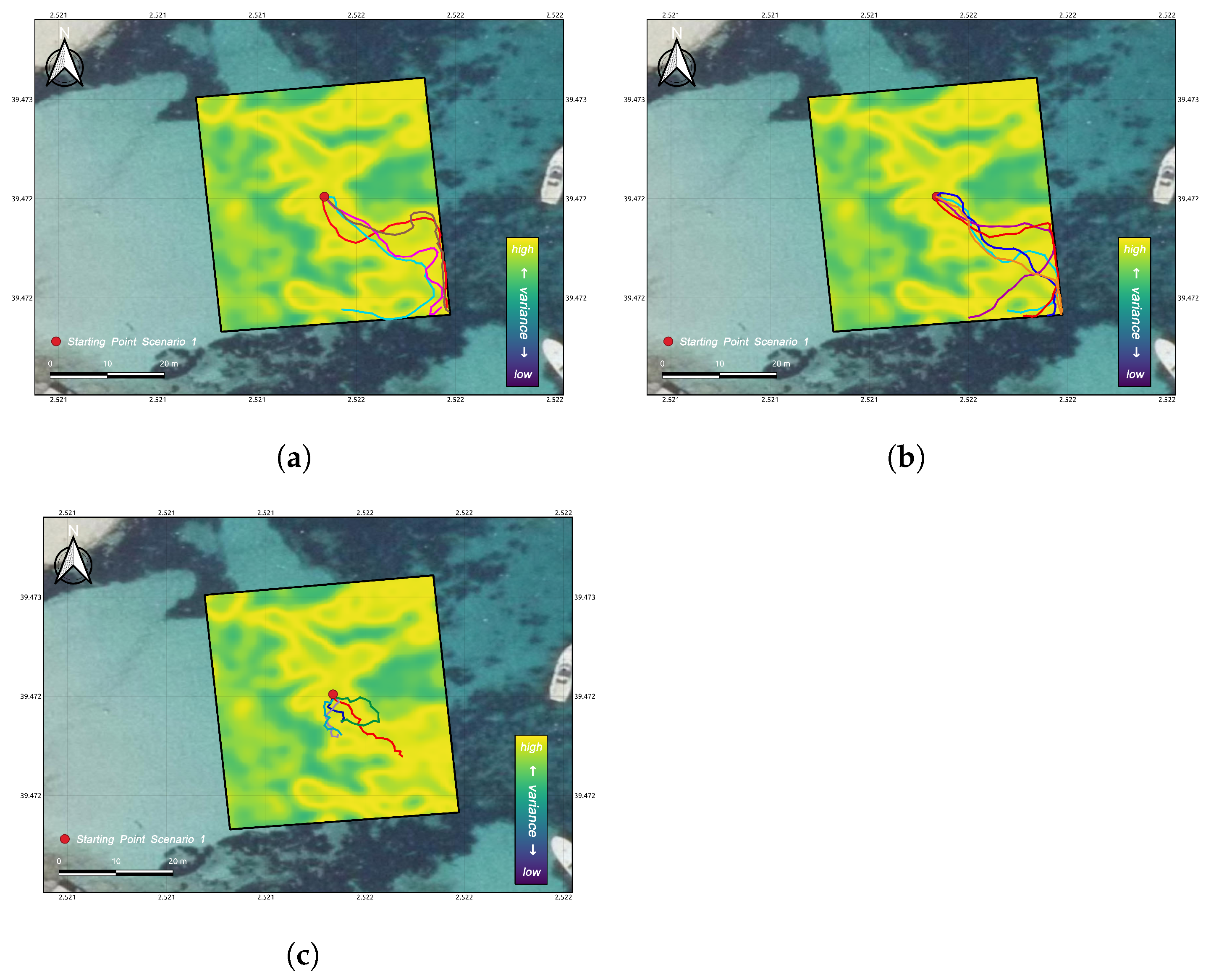
3.3. Comparative Analysis
4. Discussion
5. Conclusions
Author Contributions
Funding
Conflicts of Interest
Abbreviations
| AUV | Autonomous Underwater Vehicle |
| CNN | Convolutional Neural Network |
| DE | Differential Entropy |
| GA | Genetic Algorithm |
| GP | Gaussian Process |
| GPP | Genetic Path Planner |
| IG | Information Gathering |
| IPP | Informative Path Planning |
| ME | Mean Entropy |
| MI | Mutual Information |
| O2E | Distance Origin to End |
| PL | Path Length |
| PO | Posidonia Oceanica |
| RIG | Rapidly-exploring Information Gathering |
| RRT | Rapidly-exploring Random Tree |
| S-B | Sampling-Based Planner |
| S-E | Squared-Exponential |
Appendix A. Background
Appendix A.1. Gaussian Process
Appendix A.2. Genetic Algorithm
Appendix A.3. Crossover Methods
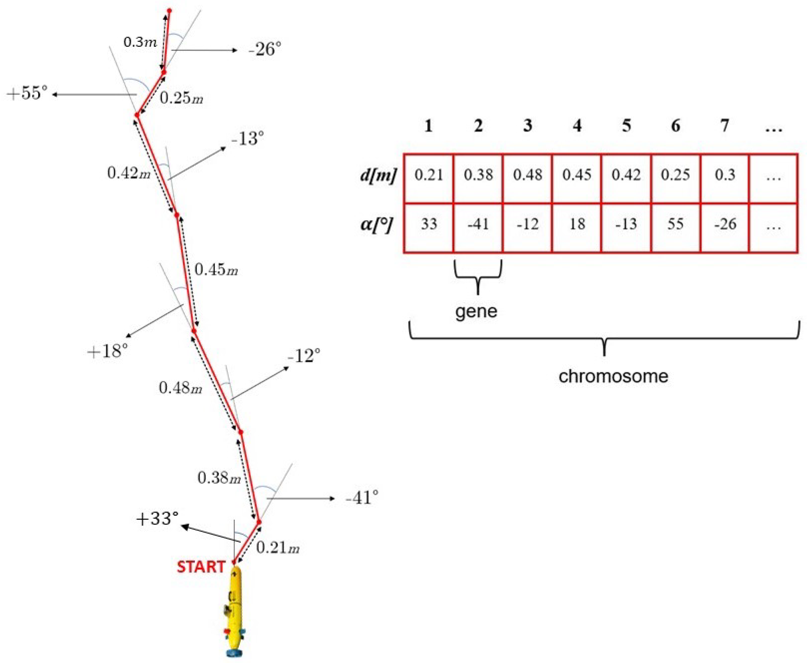
- Single-Point CrossoverThis method selects pairs of chromosomes with m genes according to their ranking order and samples from a uniform distribution with range the index of mutation . Then, the genes from to the end are switched between the pair of chromosomes. An illustration of this crossover approach is given in the Figure A1a.
- Double-Point CrossoverSimilar to the Single-Point Crossover, this method also selects a pair of chromosomes according to their ranking, but differs in that it samples two mutation indices. The first, is sampled from a uniform distribution with range ; the second, is also sampled from a uniform distribution but with range , so that . Then, the genes in the range are switched between the pair of chromosomes. Figure A1b shows an example of this crossover method.
- Uniform CrossoverThis method generates a random array with dimension m (as the number of genes in each chromosomes) sampling from an uniform distribution with range . The pair of chromosomes doing crossover, which are selected according to their ranking position, switch their genes where the value of the random array is higher or equal than a probability p. A visual example is provided in the Figure A1c, where .
- Single-Random CrossoverWorking almost as the Single-Point Crossover, this method differs only in how the pair of chromosomes are selected. In fact, differently form the previous approaches, which are based on the ranking order, in this one the chromosomes are randomly paired up. Figure A1d shows an example of this approach, where the randomly generated pairs are 3rd–9th, 4th–6th, and 5th–10th.

References
- McFarland, C.J.; Jakuba, M.V.; Suman, S.; Kinsey, J.C.; Whitcomb, L.L. Toward ice-relative navigation of underwater robotic vehicles under moving sea ice: Experimental evaluation in the arctic sea. In Proceedings of the 2015 IEEE International Conference on Robotics and Automation (ICRA), Seattle, WA, USA, 26–30 May 2015; pp. 1527–1534. [Google Scholar]
- Williams, S.B.; Pizarro, O.R.; Jakuba, M.V.; Johnson, C.R.; Barrett, N.S.; Babcock, R.C.; Kendrick, G.A.; Steinberg, P.D.; Heyward, A.J.; Doherty, P.J.; et al. Monitoring of benthic reference sites: Using an autonomous underwater vehicle. IEEE Robot. Autom. Mag. 2012, 19, 73–84. [Google Scholar] [CrossRef]
- Schofield, O.; Ducklow, H.W.; Martinson, D.G.; Meredith, M.P.; Moline, M.A.; Fraser, W.R. How do polar marine ecosystems respond to rapid climate change? Science 2010, 328, 1520–1523. [Google Scholar] [CrossRef] [PubMed] [Green Version]
- Mayer, L. Frontiers in sea floor mapping and visualization. Mar. Geophys. Res. 2006, 27, 7–17. [Google Scholar] [CrossRef]
- Furlong, M.E.; Paxton, D.; Stevenson, P.; Pebody, M.; McPhail, S.D.; Perrett, J. Autosub long range: A long range deep diving AUV for ocean monitoring. In Proceedings of the 2012 IEEE/OES Autonomous Underwater Vehicles (AUV), Southampton, UK, 24–27 September 2012; pp. 1–7. [Google Scholar]
- Raja, P.; Pugazhenthi, S. Optimal path planning of mobile robots: A review. Int. J. Phys. Sci. 2012, 7, 1314–1320. [Google Scholar] [CrossRef]
- Binney, J.; Krause, A.; Sukhatme, G.S. Informative Path Planning for an Autonomous Underwater Vehicle. In Proceedings of the 2010 IEEE International Conference on Robotics and Automation (ICRA), Anchorage, Alaska, 3–8 May 2010; pp. 4791–4796. [Google Scholar]
- Rasmussen, C.E.; Williams, C.K.I. Gaussian Processes for Machine Learning (Adaptive Computation and Machine Learning); The MIT Press: Cambridge, MA, USA, 2006. [Google Scholar]
- Krause, A.; Singh, A.; Guestrin, C. Near-optimal sensor placements in Gaussian processes: Theory, efficient algorithms and empirical studies. J. Mach. Learn. Res. 2008, 9, 235–284. [Google Scholar]
- Ma, K.C.; Liu, L.; Heidarsson, H.K.; Sukhatme, G.S. Data-driven learning and planning for environmental sampling. J. Field Robot. 2018, 35, 643–661. [Google Scholar] [CrossRef] [Green Version]
- Guerrero-Font, E.; Bonin-Font, F.; Martin-Abadal, M.; Gonzalez-Cid, Y.; Oliver-Codina, G. Sparse Gaussian process for online seagrass semantic mapping. Expert Syst. Appl. 2021, 170, 114478. [Google Scholar] [CrossRef]
- Ghaffari Jadidi, M.; Valls Miro, J.; Dissanayake, G. Sampling-based incremental information gathering with applications to robotic exploration and environmental monitoring. Int. J. Robot. Res. 2019, 38, 658–685. [Google Scholar] [CrossRef] [Green Version]
- Hollinger, G.A.; Pereira, A.A.; Sukhatme, G.S. Learning uncertainty models for reliable operation of autonomous underwater vehicles. In Proceedings of the 2013 IEEE International Conference on Robotics and Automation (ICRA), Karlsruhe, Germany, 6–10 May 2013; pp. 5593–5599. [Google Scholar]
- Viseras, A.; Shutin, D.; Merino, L. Robotic active information gathering for spatial field reconstruction with rapidly-exploring random trees and online learning of Gaussian processes. Sensors 2019, 19, 1016. [Google Scholar] [CrossRef] [PubMed] [Green Version]
- Krause, A.; Guestrin, C. Submodularity and its applications in optimized information gathering. ACM Trans. Intell. Syst. Technol. 2011, 2, 1–20. [Google Scholar] [CrossRef]
- Marchant, R.; Ramos, F. Bayesian optimisation for intelligent environmental monitoring. In Proceedings of the 2012 IEEE/RSJ International Conference on Intelligent Robots and Systems (IROS), Algarve, Portugal, 7–12 October 2012; pp. 2242–2249. [Google Scholar]
- Binney, J.; Sukhatme, G.S. Branch and bound for informative path planning. In Proceedings of the 2012 IEEE International Conference on Robotics and Automation (ICRA), Saint Paul, MI, USA, 14–18 May 2012; pp. 2147–2154. [Google Scholar]
- Kodgule, S.; Candela, A.; Wettergreen, D. Non-myopic planetary exploration combining in situ and remote measurements. arXiv 2019, arXiv:1904.12255. [Google Scholar]
- Yang, K.; Keat Gan, S.; Sukkarieh, S. A Gaussian process-based RRT planner for the exploration of an unknown and cluttered environment with a UAV. Adv. Robot. 2013, 27, 431–443. [Google Scholar] [CrossRef]
- Hollinger, G.A.; Sukhatme, G.S. Sampling-based robotic information gathering algorithms. Int. J. Robot. Res. 2014, 33, 1271–1287. [Google Scholar] [CrossRef]
- Schmid, L.; Pantic, M.; Khanna, R.; Ott, L.; Siegwart, R.; Nieto, J. An efficient sampling-based method for online informative path planning in unknown environments. IEEE Robot. Autom. Lett. 2020, 5, 1500–1507. [Google Scholar] [CrossRef] [Green Version]
- Xiong, C.; Zhou, H.; Lu, D.; Zeng, Z.; Lian, L.; Yu, C. Rapidly-Exploring Adaptive Sampling Tree*: A Sample-Based Path-Planning Algorithm for Unmanned Marine Vehicles Information Gathering in Variable Ocean Environments. Sensors 2020, 20, 2515. [Google Scholar] [CrossRef] [PubMed]
- Hitz, G.; Galceran, E.; Garneau, M.È.; Pomerleau, F.; Siegwart, R. Adaptive continuous-space informative path planning for online environmental monitoring. J. Field Robot. 2017, 34, 1427–1449. [Google Scholar] [CrossRef]
- Popović, M.; Vidal-Calleja, T.; Chung, J.J.; Nieto, J.; Siegwart, R. Informative Path Planning for Active Field Mapping under Localization Uncertainty. In Proceedings of the 2020 IEEE International Conference on Robotics and Automation (ICRA), Xi’an, China, 31 October 2020; pp. 10751–10757. [Google Scholar]
- Xiong, C.; Chen, D.; Lu, D.; Zeng, Z.; Lian, L. Path planning of multiple autonomous marine vehicles for adaptive sampling using Voronoi-based ant colony optimization. Robot. Auton. Syst. 2019, 115, 90–103. [Google Scholar] [CrossRef]
- LaValle, S.M. Rapidly-Exploring Random Trees: A New Tool for Path Planning. The Annual Research Report. 1998. Available online: https://www.semanticscholar.org/paper/Rapidly-exploring-random-trees-%3A-a-new-tool-for-LaValle/d967d9550f831a8b3f5cb00f8835a4c866da60ad (accessed on 10 October 2021).
- Yu, X.; Gen, M. Introduction to Evolutionary Algorithms; Springer: Berlin/Heidelberg, Germany, 2010. [Google Scholar]
- Katoch, S.; Chauhan, S.S.; Kumar, V. A review on genetic algorithm: Past, present, and future. Multimed. Tools Appl. 2020, 80, 8091–8126. [Google Scholar] [CrossRef]
- Kapanoglu, M.; Alikalfa, M.; Ozkan, M.; Parlaktuna, O. A pattern-based genetic algorithm for multi-robot coverage path planning minimizing completion time. J. Intell. Manuf. 2012, 23, 1035–1045. [Google Scholar] [CrossRef]
- Roberge, V.; Tarbouchi, M.; Labonté, G. Comparison of parallel genetic algorithm and particle swarm optimization for real-time UAV path planning. IEEE Trans. Ind. Informatics 2012, 9, 132–141. [Google Scholar] [CrossRef]
- Alvarez, A.; Caiti, A.; Onken, R. Evolutionary path planning for autonomous underwater vehicles in a variable ocean. IEEE J. Ocean. Eng. 2004, 29, 418–429. [Google Scholar] [CrossRef]
- Tao, W.; Yan, S.; Pan, F.; Li, G. AUV Path Planning Based on Improved Genetic Algorithm. In Proceedings of the 2020 5th International Conference on Automation, Control and Robotics Engineering (CACRE), Dalian, China, 19–20 September 2020; pp. 195–199. [Google Scholar]
- Tanakitkorn, K.; Wilson, P.A.; Turnock, S.R.; Phillips, A.B. Grid-based GA path planning with improved cost function for an over-actuated hover-capable AUV. In Proceedings of the 2014 IEEE/OES Autonomous Underwater Vehicles (AUV), Oxford, MI, USA, 6–9 October 2014; pp. 1–8. [Google Scholar]
- Li, Y.; Huang, Z.; Xie, Y. Path planning of mobile robot based on improved genetic algorithm. In Proceedings of the 2020 3rd International Conference on Electron Device and Mechanical Engineering (ICEDME), Suzhou, China, 1–3 May 2020; pp. 691–695. [Google Scholar]
- Marbà, N.; Duarte, C.M.; Cebrián, J.; Gallegos, M.E.; Olesen, B.; Sand-Jensen, K. Growth and population dynamics of Posidonia oceanica on the Spanish Mediterranean coast: Elucidating seagrass decline. Mar. Ecol. Prog. Ser. 1996, 137, 203–213. [Google Scholar] [CrossRef]
- Martin-Abadal, M.; Guerrero-Font, E.; Bonin-Font, F.; Cid, Y.G. Deep Semantic Segmentation in an AUV for Online Posidonia Oceanica Meadows Identification. IEEE Access 2018, 6, 60956–60967. [Google Scholar] [CrossRef]
- Ridolfi, A.; Costanzi, R.; Fanelli, F.; Monni, N.; Allotta, B.; Bianchi, S.; Conti, R.; Gelli, J.; Gori, L.; Pugi, L.; et al. FeelHippo: A low-cost autonomous underwater vehicle for subsea monitoring and inspection. In Proceedings of the 2016 IEEE 16th International Conference on Environment and Electrical Engineering (EEEIC), Florence, Italy, 7–10 June 2016; pp. 1–6. [Google Scholar] [CrossRef] [Green Version]
- Gelli, J.; Meschini, A.; Monni, N.; Pagliai, M.; Ridolfi, A.; Marini, L.; Allotta, B. Development and Design of a Compact Autonomous Underwater Vehicle: Zeno AUV. In Proceedings of the 11th IFAC Conference on Control Applications in Marine Systems, Robotics, and Vehicles (CAMS 2018), Opatija, Croatia, 11–12 September 2018. [Google Scholar] [CrossRef]
- Carreras, M.; Candela, C.; Ribas, D.; Palomeras, N.; Magií, L.; Mallios, A.; Vidal, E.; Pairet, È.; Ridao, P. Testing SPARUS II AUV, an Open Platform for Industrial, Scientific and Academic Applications. CoRR. 2018. Available online: https://arxiv.org/abs/1811.03494 (accessed on 10 October 2021).
- Allen, B.; Stokey, R.; Austin, T.; Forrester, N.; Goldsborough, R.; Purcell, M.; von Alt, C. REMUS: A Small, Low Cost AUV; System Description, Field Trials and Performance Results. 1997, Volume 2, pp. 994–1000. Available online: https://www.semanticscholar.org/paper/REMUS%3A-a-small%2C-low-cost-AUV%3B-system-description%2C-Allen-Stokey/e93b548c13c28548bfd22d9147abb656e435a04b (accessed on 10 October 2021).
- Sivanandam, S.; Deepa, S. Genetic algorithms. In Introduction to Genetic Algorithms; Springer: Berlin/Heidelberg, Germany, 2008; pp. 15–37. [Google Scholar]
- Cover, T.M. Elements of Information Theory; John Wiley & Sons: Hoboken, NJ, USA, 1999. [Google Scholar]
- Matthews, A.G.d.G.; van der Wilk, M.; Nickson, T.; Fujii, K.; Boukouvalas, A.; León-Villagrá, P.; Ghahramani, Z.; Hensman, J. GPflow: A Gaussian process library using TensorFlow. J. Mach. Learn. Res. 2017, 18, 1–6. [Google Scholar]
- Abadi, M.; Agarwal, A.; Barham, P.; Brevdo, E.; Chen, Z.; Citro, C.; Corrado, G.S.; Davis, A.; Dean, J.; Devin, M.; et al. TensorFlow: Large-Scale Machine Learning on Heterogeneous Systems. 2015. Available online: tensorflow.org (accessed on 10 October 2021).
- Shivgan, R.; Dong, Z. Energy-Efficient Drone Coverage Path Planning using Genetic Algorithm. In Proceedings of the 2020 IEEE 21st International Conference on High Performance Switching and Routing (HPSR), Newark, NJ, USA, 11–14 May 2020; pp. 1–6. [Google Scholar]


| Symbol | Description | Value |
|---|---|---|
| Global initialisation | ||
| n | # of chromosomes in the initial population | 200 |
| m | # of genes per chromosome | 40 |
| Std. Dev. of the Gaussian distribution of | ||
| Lower bound of the uniform distribution of d | 0.2 m | |
| Higher bound of the uniform distribution of d | 0.8 m | |
| Genetic operations | ||
| k | # of chromosomes maintained after the “Ranking” phase | 10 |
| q | Gene mutation rate | |
| z | Chromosome mutation rate | |
| Duration limit of the iterative phase | 15 s | |
| Utility function | ||
| Tuning parameter for the trade-off in the utility function | ||
| Consistency check | ||
| Attempts limit to generate from the Gaussian distributions | 10 | |
| Attempts limit to generate from the uniform distribution | 15 | |
| # of genes to delete to exit from inconsistent conditions | 5 | |
| AREA 1 (Figure 4a) | ||||
|---|---|---|---|---|
| Scenario | Planner | ME [bits] | PL [m] | O2E [m] |
| First | Genetic | |||
| Random | ||||
| S-B | ||||
| Second | Genetic | |||
| Random | ||||
| S-B | ||||
| Third | Genetic | |||
| Random | ||||
| S-B | ||||
| AREA 2 (Figure 4b) | ||||
|---|---|---|---|---|
| Scenario | Planner | ME [bits] | PL [m] | O2E [m] |
| First | Genetic | |||
| Random | ||||
| S-B | ||||
| Second | Genetic | |||
| Random | ||||
| S-B | ||||
| Third | Genetic | |||
| Random | ||||
| S-B | ||||
| AREA 3 (Figure 4c) | ||||
|---|---|---|---|---|
| Scenario | Planner | ME [bits] | PL [m] | O2E [m] |
| First | Genetic | |||
| Random | ||||
| S-B | ||||
| Second | Genetic | |||
| Random | ||||
| S-B | ||||
| Third | Genetic | |||
| Random | ||||
| S-B | ||||
| AREA 1 | ||
|---|---|---|
| Scenario 1 | Scenario 2 | Scenario 3 |
| Genetic: | Genetic: | Genetic: |
| Random: | Random: | Random: |
| S-B: | S-B: | S-B: |
| AREA 2 | ||
| Scenario 1 | Scenario 2 | Scenario 3 |
| Genetic: | Genetic: | Genetic: |
| Random: | Random: | Random: |
| S-B: | S-B: | S-B: |
| AREA 3 | ||
| Scenario 1 | Scenario 2 | Scenario 3 |
| Genetic: | Genetic: | Genetic: |
| Random: | Random: | Random: |
| S-B: | S-B: | S-B: |
Publisher’s Note: MDPI stays neutral with regard to jurisdictional claims in published maps and institutional affiliations. |
© 2021 by the authors. Licensee MDPI, Basel, Switzerland. This article is an open access article distributed under the terms and conditions of the Creative Commons Attribution (CC BY) license (https://creativecommons.org/licenses/by/4.0/).
Share and Cite
Bresciani, M.; Ruscio, F.; Tani, S.; Peralta, G.; Timperi, A.; Guerrero-Font, E.; Bonin-Font, F.; Caiti, A.; Costanzi, R. Path Planning for Underwater Information Gathering Based on Genetic Algorithms and Data Stochastic Models. J. Mar. Sci. Eng. 2021, 9, 1183. https://doi.org/10.3390/jmse9111183
Bresciani M, Ruscio F, Tani S, Peralta G, Timperi A, Guerrero-Font E, Bonin-Font F, Caiti A, Costanzi R. Path Planning for Underwater Information Gathering Based on Genetic Algorithms and Data Stochastic Models. Journal of Marine Science and Engineering. 2021; 9(11):1183. https://doi.org/10.3390/jmse9111183
Chicago/Turabian StyleBresciani, Matteo, Francesco Ruscio, Simone Tani, Giovanni Peralta, Andrea Timperi, Eric Guerrero-Font, Francisco Bonin-Font, Andrea Caiti, and Riccardo Costanzi. 2021. "Path Planning for Underwater Information Gathering Based on Genetic Algorithms and Data Stochastic Models" Journal of Marine Science and Engineering 9, no. 11: 1183. https://doi.org/10.3390/jmse9111183
APA StyleBresciani, M., Ruscio, F., Tani, S., Peralta, G., Timperi, A., Guerrero-Font, E., Bonin-Font, F., Caiti, A., & Costanzi, R. (2021). Path Planning for Underwater Information Gathering Based on Genetic Algorithms and Data Stochastic Models. Journal of Marine Science and Engineering, 9(11), 1183. https://doi.org/10.3390/jmse9111183