Artificial Intelligence Search Strategies for Autonomous Underwater Vehicles Applied for Submarine Groundwater Discharge Site Investigation

Abstract

In this study, a set of different search strategies for locating submarine groundwater discharge (SGD) are investigated. This set includes pre-defined path planning (PPP), adapted random walk (RW), particle swarm optimisation (PSO), inertia Levy-flight (ILF), self-organising-migration-algorithm (SOMA), and bumblebee search algorithm (BB). The influences of self-localisation and communication errors and limited travel distance of the autonomous underwater vehicles (AUVs) on the performance of the proposed algorithms are investigated. This study shows that the proposed search strategies could not outperform the classic search heuristic based on full coverage path planning if all AUVs followed the same search strategy. In this study, the influence of self-localisation and communication errors was investigated. The simulations showed that, based on the median error of the search runs, the performance of SOMA was in the same order of magnitude regardless the strength of the localisation error. Furthermore, it was shown that the performance of BB was highly affected by increasing localisation errors. From the simulations, it was revealed that all the algorithms, except for PSO and SOMA, were unaffected by disturbed communications. Here, the best performance was shown by PPP, followed by BB, SOMA, ILF, PSO, and RW. Furthermore, the influence of the limited travel distances of the AUVs on the search performance was evaluated. It was shown that all the algorithms, except for PSO, were affected by the shorter maximum travel distances of the AUVs. The performance of PPP increased with increasing maximum travel distances. However, for maximum travel distances > 1800 m the median error appeared constant. The effect of shorter travel distances on SOMA was smaller than on PPP. For maximum travel distances < 1200 m, SOMA outperformed all other strategies. In addition, it can be observed that only BB showed better performances for shorter travel distances than for longer ones. On the other hand, with different search strategies for each AUV, the search performance of the whole swarm can be improved by incorporating population-based search strategies such as PSO and SOMA within the PPP scheme. The best performance was achieved for the combination of two AUVs following PPP, while the third AUV utilised PSO. The best fitness of this combination was 15.9. This fitness was 26.4% better than the performance of PPP, which was 20.4 on average. In addition, a novel mechanism for dynamically selecting a search strategy for an AUV is proposed. This mechanism is based on fuzzy logic. This dynamic approach is able to perform at least as well as PPP and SOMA for different travel distances of AUVs. However, due to the better adaptation to the current situation, the overall performance, calculated based on the fitness achieved for different maximum travel distances, the proposed dynamic search strategy selection performed 32.8% better than PPP and 34.0% better than SOMA.

1. Introduction

Autonomous underwater vehicles (AUVs) are untethered underwater vehicles that follow a pre-defined route or use a real-time adaptive mission control system [1]. AUVs can also be defined as robotic systems equipped with a propulsion system and an on-board computer for decision making [2]. AUVs can be utilised for various different tasks, including bathymetry surveys [3], harbour inspections [4], data mulling [5], water quality analysis [6], tracking of upwelling fronts [7], or chemical plume tracing [8,9]. Detailed reviews on recent developments in the different AUV-related fields are given in [2,10,11].

AUVs are suitable for accelerating the speed of surveys and allow the gathering of coherent data using side scan sonars, for example [3]. Surveys carried out by human divers are often too dangerous, due to the imminent risk of shark or crocodile attacks [12]. Schlüter et al. [13] utilised an AUV during a survey on submarine groundwater discharge (SGD) sites in the Baltic sea. To create high-resolution benthic maps, the AUV utilised a side scan sonar. It was also equipped with a combined sensor to measure the conductivity, temperature, and the depth (CTD). However, the AUV was not able to detect freshwater from the SGD using the CTD [13].

During their missions, AUVs usually follow a pre-defined path, such as a series of different transects defined by waypoints [3,12], or an adaptive sampling strategy [10,14], to achieve a given goal. Behaviour-based planning (BBP) is one instance of an adaptive sampling strategy. BBP is a bottom-up approach, tailoring intelligent behaviour utilising simple features [8]. In BBP, the term behaviour describes an algorithm, which maps sensor inputs to a pattern of motor actions. Usually, different behaviours are implemented, requiring a coordinating mechanism to choose the right behaviour [8]. BBP is regularly used for chemical plume tracking [8,15,16,17,18,19,20]. Formation control methods, such as leader-follower approaches, are often used to control the behaviour of individual AUVs when a group of AUVs is utilised [21].

Another possible solution is the application of population-based optimisation algorithms such as particle swarm optimisation (PSO) [22] or ant colony optimisation (ACO) [23] to guide a group of AUVs during a search mission [24]. In recent research, PSO was proposed as a potential search algorithm for odour source localisation [25,26]. Different algorithms can be implemented on the AUVs and used as different behaviours in a BBP. However, in this case, a coordinating mechanism, deciding on the right search strategy, is required. Fuzzy logic [27] can be used to decide on the right search algorithm.

Regularly, the approach suggested by Mamdani [28] is used to build fuzzy logic systems. In his approach, the rule base, provided by an expert, is given as a set of if-then statements [29]. The utilisation of fuzzy logic requires the definition of a number of membership functions (MFs) for all inputs and outputs, and a set of rules operating on the defined MFs of the input variables, calculating the output value. In the past, fuzzy logic was applied to a vast number of problems in a variety of different fields. This includes: control-theory [28], crack detection in beams [30], fire detection in engines and batteries [31], pavement section classification [32], characterisation of large changes in wind power [33] path planning and obstacle avoidance of mobile unmanned robots [34,35], and analysing the effect of traffic noise on the human work efficiency [29]. Recently, fuzzy logic has been used to detect SGD plumes from multi-sensor data [36].

The term SGD covers any flow of water out across the seabed to the coastal ocean on continental margins, regardless of the composition and the driving force [37,38]. In general, groundwater can discharge either via submarine springs or via disseminated seepages [37]. SGDs are recognised as important pathways for nutrients and pollutions to the marine environment [39,40]. Therefore, marine scientists are interested in the localisation and investigation of SGD sites.

Different methods, such as seepage meters [41,42,43], tracer studies [37], remote sensing [44], or seismic surveys [45,46,47], were utilised for SGD investigation in the past. The majority of these methods focused either on the aquifer or on the mixing of the discharged water on larger scales.

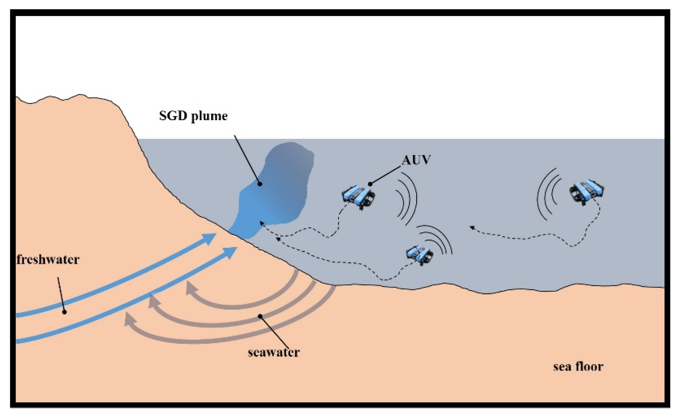
In a recent study [36], small underwater vehicles, guided by a human pilot, are utilised for the investigation of SGD sites. However, if a human pilot guides the vehicle, these investigations are labour-intensive. Hence, AUVs could be a potential tool for SGD investigations. Due to the sizes of the areas under investigation, utilising a small swarm of AUVs would potentially be more suitable than the application of a single AUV. Furthermore, the AUVs must be guided by a search strategy. As mentioned above, coverage path planning algorithms are usually utilised for these kinds of missions. However, artificial intelligence optimisation algorithms can be used to improve the search performance of a swarm of AUVs. In this paper, different search strategies for SGD detection are proposed and their performances are evaluated. It is assumed that population-based optimisation algorithms can improve the performance of a swarm of AUVs. These algorithms can be used to generate new waypoints based on the information gathered from the environment. In this study, the AUVs are independent agents, each following its own search pattern. However, the AUVs are able to communicate with the other entities in the swarm to exchange search information. Based on the search strategy, this information is utilised during the search. A sketch summarising the concept of a small swarm searching for a SGD plume is shown in Figure 1.

It was shown in this comprehensive study that the proposed algorithms offer the potential to enable automated explorations of SGD sites utilising AUVs. The remainder of this paper is structured as follows. In Section 2, the dynamic simulation environment used as a testbed for the search is presented. The different search strategies investigated in this research are introduced in Section 3. In Section 4, the different simulations carried out are described. The results of the experiments are presented in Section 5. A discussion of the findings can be found in Section 6. Section 7 draws this paper to a conclusion.

2. Environmental Simulation as Testbed for Search Algorithms

For the evaluation of the capabilities of search algorithms, an environmental simulation is required as fitness function. In recent research, different kinds of fitness functions, such as cellular automata [24], static conductivity distributions [48] or static plateau functions [49], were used for evaluating the performance of different search strategies. However, all of these fitness functions lack similarity to the real world. Hence, in this study, a novel environmental simulation, based on real-world measurement data, was developed. The simulation is based on the findings of an environmental study, which took place in the Northern Harbour of the Woodman Point area near Perth (Western Australia). The area is connected to the Cuckburn Sound, a sheltered area between Garden Island and the Australian Mainland (Figure 2a). The water depth in the Northern Harbour varies between two and ten metres. Starting from the north end of the harbour, the water depth remains relatively constant between two and four metres. However, at a distance between 80 m and 100 m from the shore, the water depth increases from a couple of metres to ten metres. Due to the change in the hydraulic conditions, this sharp brim is expected to facilitate the development of focused SGD spots. A bathymetry map of the harbour is presented in Figure 2b.

The harbour was surveyed using an echo sounder-equipped skiff as well as a sensor equipped remotely operated vehicle (ROV). During the sonar survey, the area under investigation was covered by 13 transects (Figure 2c). The data collection was focused on the area of the brim. During these transects, georeferenced acoustic backscatter data were recorded using an Humminbird 898 SI echo-sounder [50]. The ROV was operated from three different positions to survey the whole harbour area. The positions are marked in Figure 2d. In addition, the areas in which the ROV surveys took place are marked by polygons.

During the sonar transects, 23 plumes were identified as SGD plumes. Analysing the spatial appearance of these plumes showed that the discharged water did not reach the surface; rather, it remained in water depths between approximately 1.5 and 3.0 m (Figure 3). Previous research conducted in the same harbour concludes that the discharged water was brackish, containing a huge portion of recirculating seawater [46]. Therefore, the density difference between discharged water and seawater might be small. In addition, the temperature depth profile indicated a surface layer of warmer water starting from the sea surface to a water depth of 3 to 5 m [36]. This higher temperature causes a lower density of the surface layer. This lower-density surface layer prevents the plumes from reaching the surface.

Furthermore, Figure 4 shows that the detected plumes form a connected patch. The size of the patch was approximately 75 m × 40 m. It can be observed from Figure 4 that Echograms from sonar transects passing near the patch did not show any evidence of a plume. Moreover, most plumes seem to be on the area of the brim, developing in the deeper part of the harbour.

If the plume is located at a specific depth, or at a constant distance from the seafloor, this information can be utilised during the search. The AUV, for instance, can be operated at a specific depth, using a pressure sensor, or at a specific altitude, using an echo sounder. Therefore, the search problem can be viewed as a two-dimensional search problem. Hence, a dynamical two-dimensional search space, covering the whole harbour area, was used in this study. Reducing the number of dimensions to simplify the search task of AUVs is a commonly used approach, both for simulations [52,53] and search missions in the real world [8].

The distribution of the discharged water was modelled using a simplified time-based simulation. The implemented simulation needs to run several thousands of times during the different experiments. Therefore, due to computational limitations, neither a hydrodynamic model nor other computational fluid models were used in this study. The simulation was designed to build a dynamic search environment for testing different kinds of search strategies for AUVs. The shape of the search area was chosen as a polygon for a simplified representation of the real harbour. The size of the search space was 330 m × 200 m. In addition, an area of 79 m × 36 m was defined as the SGD area; e.g., in this area, SGDs could occur. The position of the left corner of the SGD area was (81 m, 57 m). Figure 5 shows the shape and size of the designated search space, including the SGD area and the starting point of the AUVs.

Recent research revealed a dependency of SGD flowrates on the tidal cycle [46,54,55]. Therefore, the simulation developed was extended by the time-dependent inflow rate of the SGDs. Furthermore, due to tide-introduced currents, the direction of the plumes is influenced by the tide; i.e., during rising tide, the plumes are directed north-westwards, while, during low-tide, the plumes are directed south-eastwards.

The simulation contains an adjustable number of SGD spots. Once the simulation is set up, the positions of the SGDs are chosen randomly within the designated SGD area. Later, the flowrate parameter $\beta$ of each SGD is chosen randomly from the interval:

$$\left\{{\beta }_i \in ℝ | 0.1 \le {\beta }_i \le 0.5\right\}.$$

(1)

The water discharged in the area under investigation is brackish, containing a variable portion of fresh groundwater and recirculating seawater [46]. The percentage of fresh groundwater can vary depending on different factors, such as precipitation, season or other effects [56,57]. The composition of the discharged water can also vary over time. Hence, in the simulation, the weight percentage of fresh groundwater $w$ is chosen randomly for each SGD from the interval:

$$\left\{w_i \in ℝ | 0 \le w_i \le 1\right\}.$$

(2)

Next, the parameter values of the discharged water for each SGD are calculated as follows:

$$V_{SGD}=V_{FW}·w_i+V_{SW}·\left(1-w_i\right).$$

(3)

where $V_{SGD}$ represents the parameter value of the discharged water, $V_{FW}$ denotes the parameter value of the fresh groundwater, and $V_{SW}$ represents the parameter value of the recirculating seawater. Equation (3) can be used to calculate discharge values for different parameters. However, in this study, dissolved oxygen (DO) is utilised as tracer for SGDs. DO is usually depleted in groundwater [58,59]. Hence, in this simulation, the DO value of fresh groundwater is set to $V_{FW,DO}=0\frac{\mathrm{mg}}{\mathrm{l}}$. However, enriched DO values in pore water samples, potentially caused by seawater intrusion, are reported in recent research [60]. Therefore, the DO value of recirculating seawater is set to $V_{SW,DO}=8.9\frac{\mathrm{mg}}{\mathrm{l}}$. 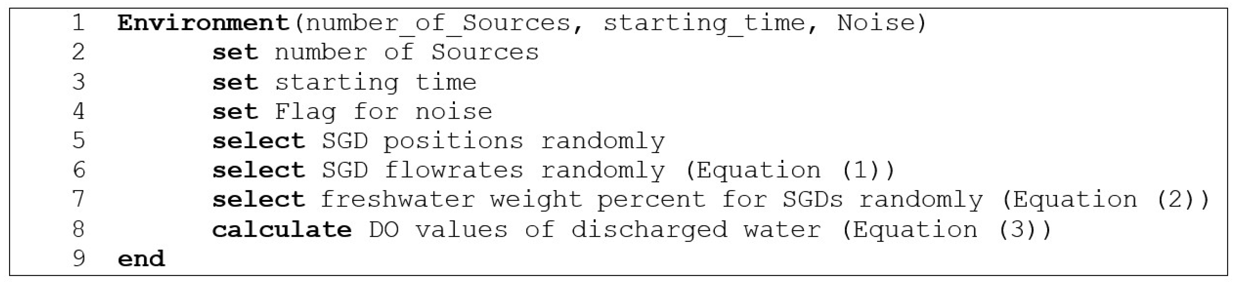This value is equal the mean DO level measured during the ROV surveys [36]. The aforementioned calculations are executed during the initialisation of the environment. Figure 6 shows the pseudocode of the constructor of the environment class.

After initialisation, the environmental simulation offers a measurement interface, which allows the AUVs to sense the environment. The interface accepts a position, given as x and y coordinates, as input parameter. The current DO value for the given position is than calculated and returned by the environment class. The Euclidean distances d_i and the angle ${\alpha }_i$ between the positons of the SGDs and the given position are calculated. Next, the flow direction of the plumes $\delta$ is calculated as follows:

$$\delta =\{\begin{array}{c}120°+2·r_n ;\mathrm{if} \mathrm{rising} \mathrm{tide} \hfill \\ 300°+2·r_n ;\mathrm{if} \mathrm{falling} \mathrm{tide}\hfill \end{array}.$$

(4)

where $\delta$ denotes the flow direction of the plumes and $r_n$ denotes a Gaussian distributed random number with mean of zero and standard deviation of one. The standard values are chosen based on the position of the harbour entry (Figure 2a). In the next step, calculated angles ${\alpha }_i$ are compared with the calculated flow direction $\delta$. The angles outside the flow area of the plume are set to 90°. The flow area is calculated based on the flow direction $\delta$ and the flow angle $\Delta \delta$. The flow angle $\Delta \delta$ changes over time, based on the tidal cycle. In addition, if the calculated distance d_i is zero, the corresponding angle ${\alpha }_i$ is set to a value of zero. Furthermore, the inflow rate of the SGDs depends on the tidal cycle. Hence, a time factor $\tau$ is calculated and used for the regulation of the inflow over time as follows:

$$\tau =\sin \left(T·t\right)+2+\Delta S\left(t\right).$$

(5)

where T denotes the period of the tide, t represents the current time of the simulation, and $\Delta S$ denotes a turn of tide parameter. This parameter changes over time, adjusting the width of the plume around the turn of tide. The parameter $\tau$ allows the dynamic change of the inflow over time, simulating the tide dependency. Figure 7 depicts the development of the parameter $\tau$ over time. It shows that the turn of tide parameter $\Delta S$ only exerts an influence on the parameter $\tau$ during the turn of the tide.

Based on the noise flag (Figure 6), the base DO value V₀ is chosen to be:

$$V_0=\{\begin{array}{c}\overline{V}+r_n·{\widehat{\sigma }}_{\overline{x}} ;\mathrm{if} \mathrm{Noise}=\mathrm{true}\\ \overline{V} ;\mathrm{if} \mathrm{Noise}=\mathrm{false}\end{array}.$$

(6)

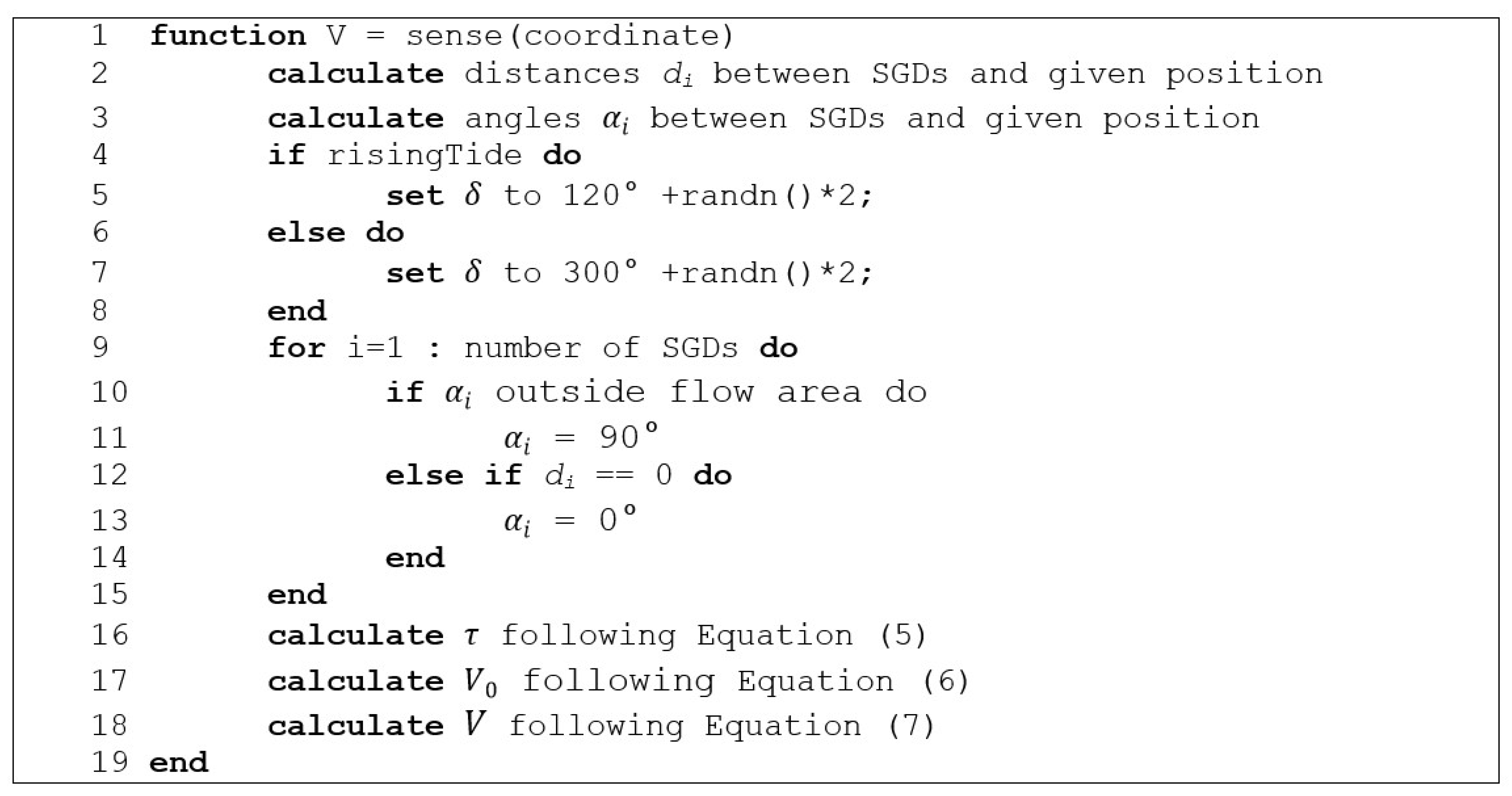
where $\overline{V}$ denotes the mean DO value measured during the ROV survey, $r_n$ denotes a Gaussian distributed random number with a mean of zero and a standard deviation of one, and ${\widehat{\sigma }}_{\overline{x}}$ represents the standard error of the mean, based on the DO values measured during the ROV survey [36]. Consequently, the DO value V for the given position is calculated as follows:

$$V=V_0+\underset{}{\min }\left(\cos \left({\alpha }_i\right)·\left(V_{SGD,i}-\overline{V}\right)·e^{-{\beta }_i·{\tau }^2·d_i}\right).$$

(7)

The sensing procedure, described above, is summarised in the pseudocode, presented in Figure 8.

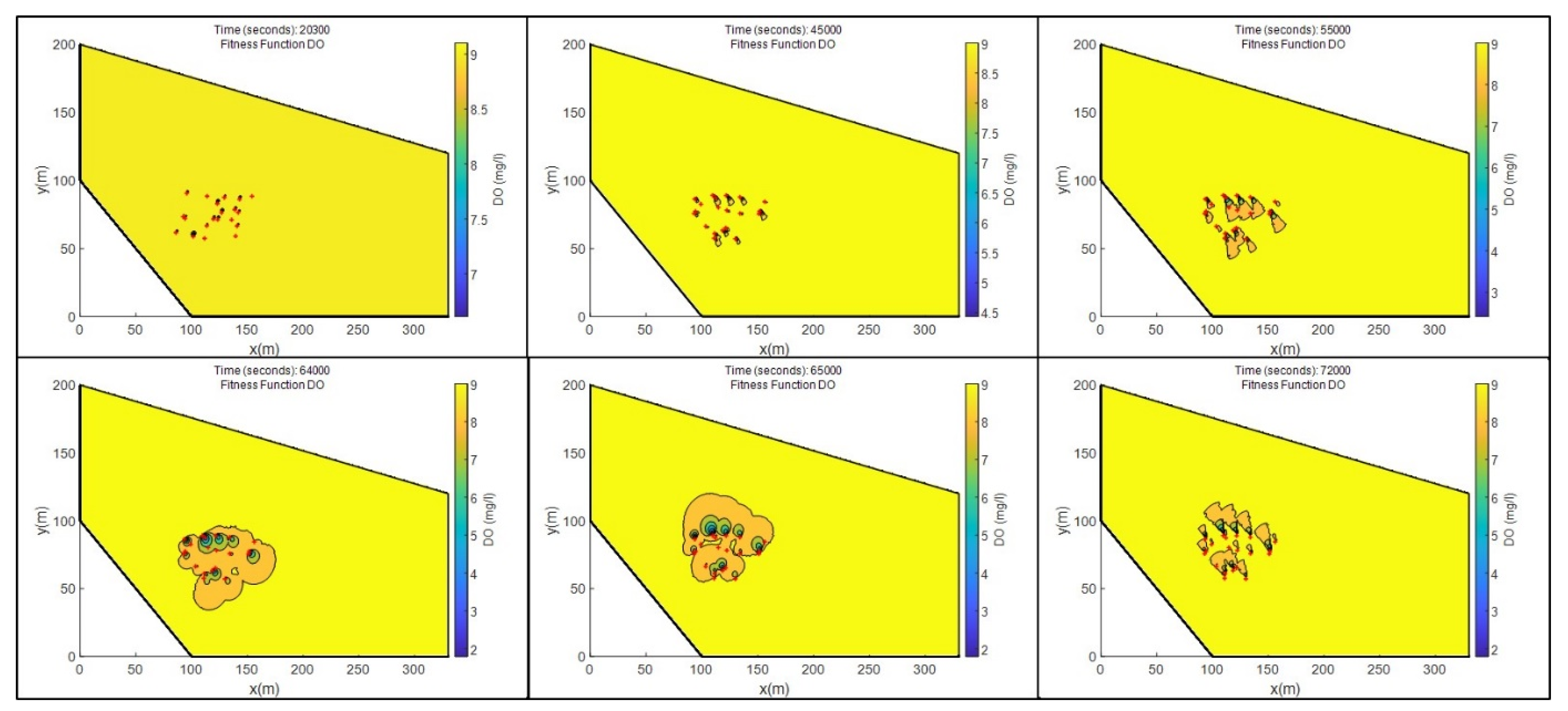
Figure 9 shows the development of the plumes over different time steps. It can be observed that the size of the different plumes varied over time. During the turn of the tide, the flow direction of the plumes changed. Furthermore, it can be observed that the plumes from the different SGDs differed in size and intensity, due to different values of the parameters ${\beta }_i$ and $w_i$. In addition, a video of the simulation environment, covering a complete tidal cycle, can be found in Supplementary Material Video S1.

2.1. Sensor Error Model

During the survey, the AUV was equipped with a low-cost sensor for measuring DO values [36]. The measurement accuracy of the sensor, as given by the manufacturer, is ${\sigma }_S=0.05\frac{\mathrm{mg}}{\mathrm{l}}$, while the measurement range of the sensor is 0.01 mg/L to 100 mg/L [61]. The sensor operates at a measurement frequency of 1 Hz. In the simulation, the sensor reading V_s is modelled as follows:

$$V_S=V+r_n·{\sigma }_S.$$

(8)

where $V$ denotes the current concentration calculated following Equation (7), $r_n$ generates a random number from the normal distribution with a mean of zero and a standard deviation of 1, and ${\sigma }_S$ denotes the measurement accuracy of the sensor.

2.2. Localisation Error Model

The use of AUVs requires a method for the robust, reliable, and accurate determination of an AUV’s position. Autonomous vehicles usually rely on the availability of global navigation satellite systems (GNSS) in order to estimate their global position. However, the electromagnetic signals of such satellite systems cannot be received by submerged AUVs [62]. Different possible methods for the localisation of submerged AUVs have been proposed. These methods can be classified into inertial or dead reckoning methods, acoustic methods, and geophysical methods [63]. All localisation methods are subject to error, whereby the respective magnitude of the error depends on both the method itself as well as other factors, for instance environmental factors. Therefore, it is not an easy task to estimate the magnitude of the localisation error. However, different strengths of localisation error can influence the performance of different search strategies [64,65]. Hence, two simplified localisation error models were used in this study, to study the impact of localisation errors on the performance of the search. The first model used a normal distributed error added to the current true position of the AUV as follows:

$$\left(\begin{array}{c}\widehat{x}\\ \widehat{y}\end{array}\right)=\left(\begin{array}{c}x+r_n·\sigma \\ y+r_n·\sigma \end{array}\right).$$

(9)

where $\widehat{x}$ and $\widehat{y}$ represent the estimated position, $x$ and $y$ denote the true position of the AUV, $r_n$ is a random number generated from the standard normal distribution with a mean of 0 and a standard deviation of 1, and $\sigma$ represents the standard deviation of the localisation. Higher values of $\sigma$ increase the uncertainty of the localisation model. By only changing a single parameter, this model can be used to represent different localisation accuracies. Hence, the model is suitable for studying the impact of localisation errors on different search strategies.

However, with acoustic-based localisation methods, the localisation error is affected by the distance between the receivers and transmitters of the localisation system [66,67]. The influence of this distance is taken into account in the second model. Here the estimated position can be calculated as follows:

$$\left(\begin{array}{c}\widehat{x}\\ \widehat{y}\end{array}\right)=\left(\begin{array}{c}x+r_n·({\sigma }_0+\sigma \left(d\right)·d\\ y+r_n·({\sigma }_0+\sigma \left(d\right)·d\end{array}\right).$$

(10)

where $\widehat{x}$ and $\widehat{y}$ represent the estimated position, $x$ and $y$ denote the true position of the AUV, $r_n$ is a random number drawn from the standard normal distribution, ${\sigma }_0$ represented the minimum standard deviation, $\sigma \left(d\right)$ represents the distance based standard deviation of the localisation model, and $d$ denotes the Euclidean distance between the AUV and the centre-point of the localisation system. This position was chosen to be at location (250, 130) m. This model was used in all the simulations, unless otherwise noted.

2.3. Communication Error Model

Underwater communication suffers from various detrimental physical effects, such as propagation loss, absorption loss, multi-path propagation, and temperature and pressure-dependent sound velocity [68]. In a real underwater environment, the reliability of a communication link is also influenced by the currently three-dimensional orientation of each communication system (i.e., transmitting and receiving AUV) as the acoustic transducers exhibit a directional response pattern. Commercial acoustic modems apply spread spectrum techniques and OFDM (orthogonal frequency division multiplex) modulation schemes in order to cope with the frequency-selective impairments of multi-path propagation. These methods make it possible to maintain a reliable communication link. On the other hand, they potentially lead to a reduced data rate (automatic rate adaption).

An adapted version of the transmission loss function of underwater acoustic systems [69] is used in this study. Here, the considered impairments are restricted to the propagation loss L_P:

$$L_P=\alpha ·10·\log \left(\frac{d}{d_0}\right).$$

(11)

where $\alpha$ denotes the damping coefficient, $d$ denotes the Euclidean distance between two AUVs, and $d_0$ represents the reference distance for normalising the path loss. Based on this loss, a probability p_com for successful communication between two AUVs can be derived as follows:

$$p_{com}=100\%-L_P.$$

(12)

It can be seen from Equation (11) that the probability of a successful communication only depends on the damping coefficient $\alpha$ and the normalising distance parameter $d_0$. Therefore, this model is suitable to study the impact of communication restrictions on the performance of different search strategies. The proposed model was used in previous research [65].

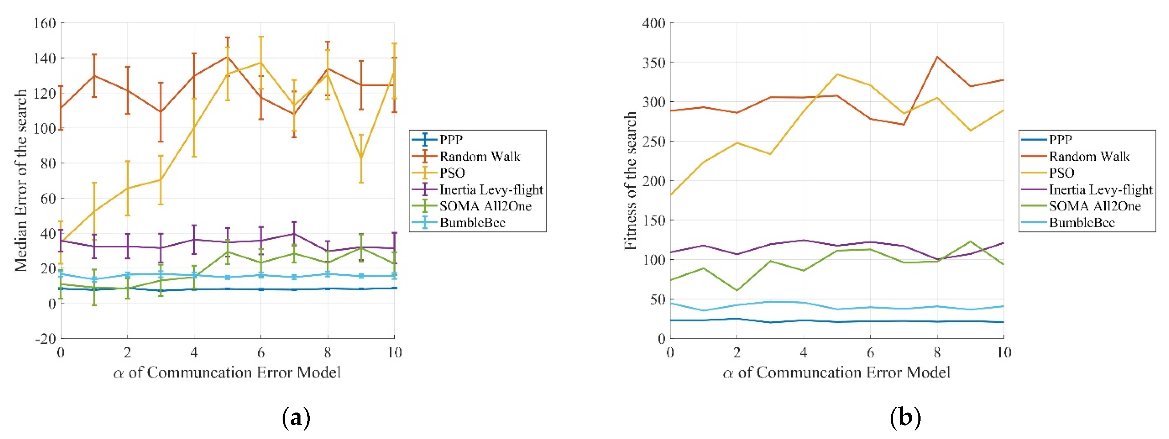
Figure 10 shows the probability of a successful communication as function of the distance between two AUVs for a variation of $\alpha$ and for different values of $d_0$. It can be observed that the influence of the damping coefficient $\alpha$ is more dominant than the influence of different values of the normalisation factor $d_0$.

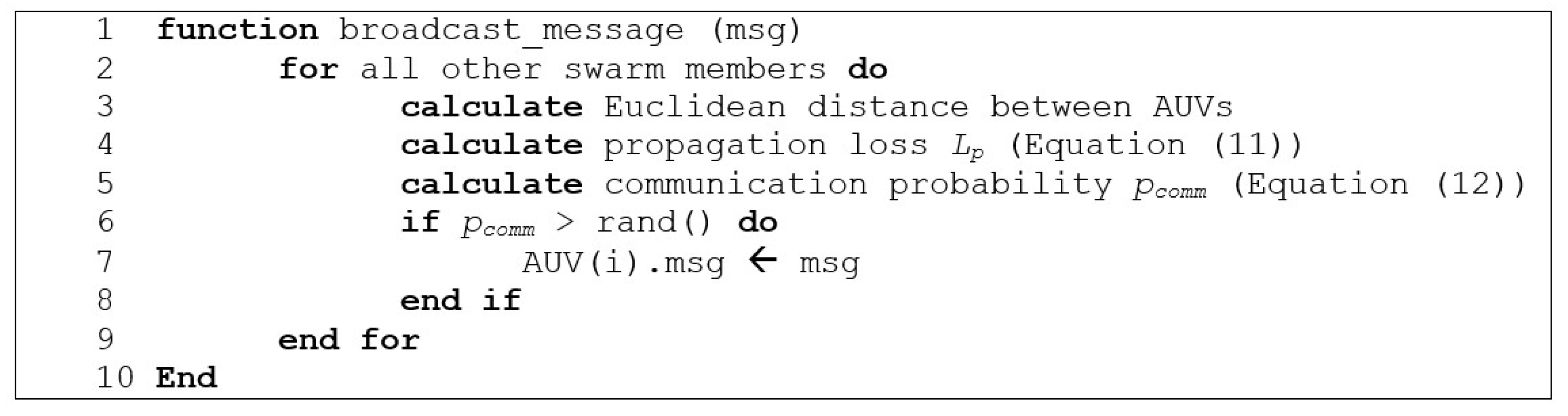
During the simulations, the AUVs are able to broadcast messages to the other members of the swarm. After an AUV sends a message, the environment computes whether the message will be received by another AUV or not. If the communication is successful, the message reaches the AUV in the next iteration. Otherwise the message is dropped. Due to bandwidth limitations, the sender does not receive any feedback about the success of the communication. The pseudocode of the communication method, implemented within the environment, is shown in Figure 11. This function is called by an AUV during the search if it tries to send a message to its peers.

3. Search Strategies Used for SGD Detection

A swarm of AUVs must be guided by a search strategy [70], which should be able to achieve the intended search goal within the limitations of the AUVs. For instance, the search strategy could exploit information gained from the environment to amend the planned search path of an AUV. However, the search strategies developed only generate waypoints for the AUV to visit. They are not responsible for other tasks, such as path planning, obstacle avoidance, or motion control. 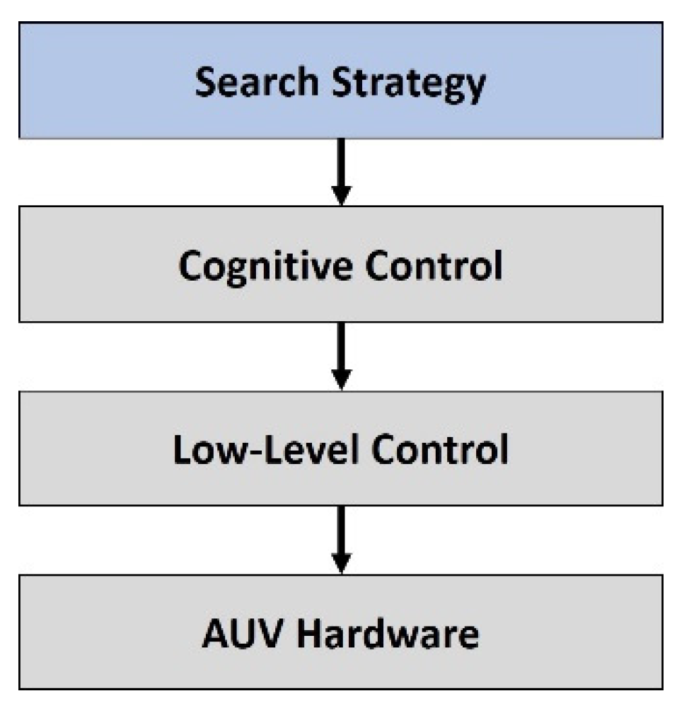Figure 12 shows the different layers involved during an AUV search task. The lowest layer contains the AUV hardware, including, for example, hardware for propulsion, energy management or sensors. The next layer is the low-level control layer. This layer contains different controllers, for example, for depth or speed control. Different kinds of controllers, such as PID controllers or Fuzzy controllers, have been used [2]. The inputs for the different low-level controllers are generated within the cognitive control layer. In addition, this layer is in charge of obstacle avoidance and optimal path planning of the AUV. The highest layer contains the search strategy, responsible for waypoint generation based on search strategies used and environmental information gained. This study contributes to this last layer; therefore, it is assumed that a swarm of AUVs, equipped with suitable systems for communication, self-localisation and environmental sensors, is available.

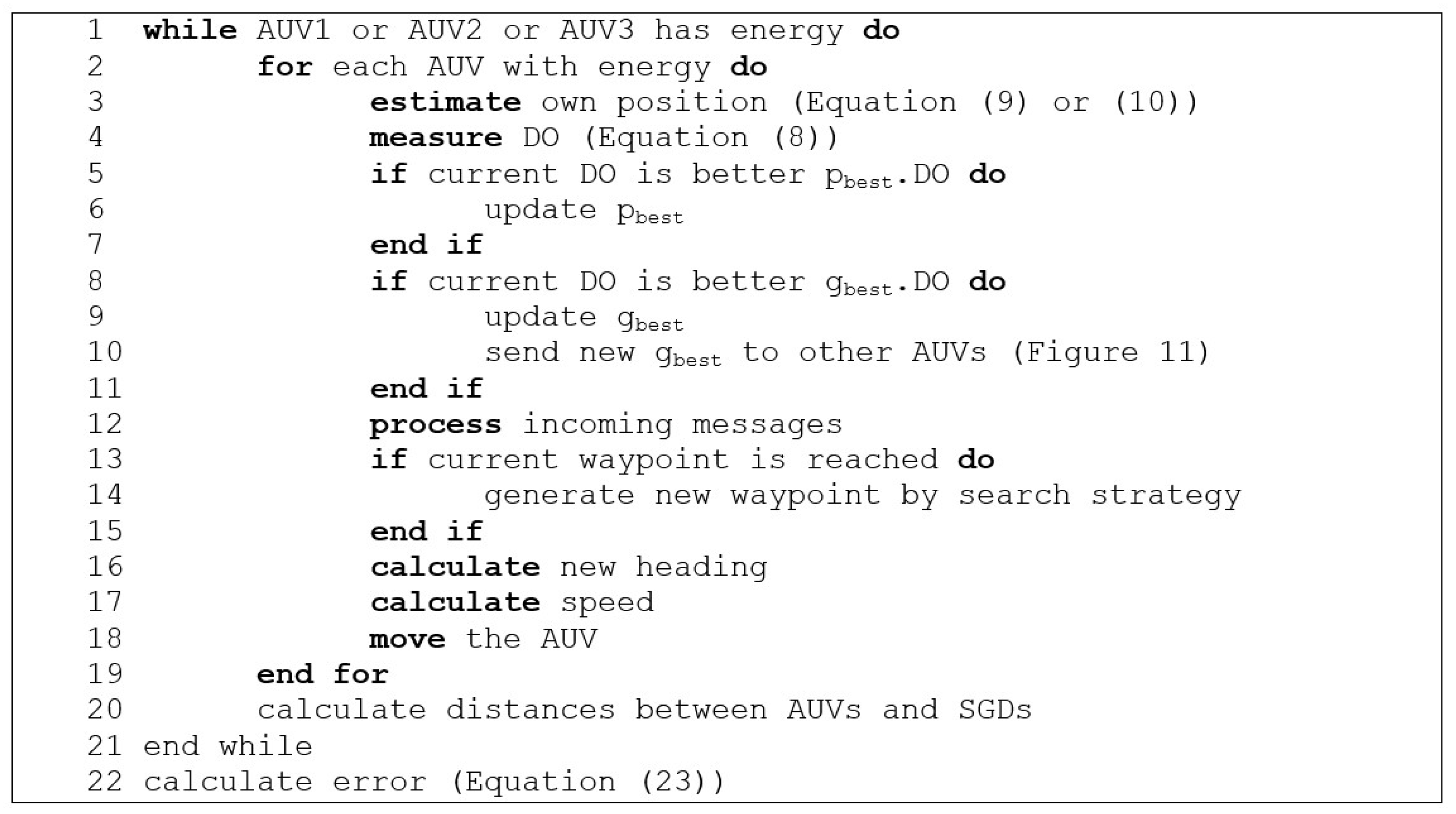
In this study, all the strategies are implemented to calculate new waypoints for the AUVs. During the simulations, in each iteration, the generated waypoints were used to calculate the desired course and speed of the AUV. These calculations are based on the estimated position of the AUV and the position of the current waypoint. Once an AUV reaches the current waypoint, the search strategies generate the next waypoint and returns it to the cognitive control layer of the AUV. In each iteration, an AUV first estimates its own position. Afterwards, it senses the environment and updates its own knowledge base, i.e., the best position found so far by the AUV (p_best) and the best position found so far by the entire swarm (g_best).

Next, the AUV processes incoming messages from the other AUVs. If the current waypoint is reached, a new position is calculated based on the search strategy used. Next, the new desired heading and speed of the AUV is calculated and the AUV moves. This behaviour continues until the maximum travel distance of all the AUVs is exceeded. During the simulations, all the AUVs in the swarm were operated simultaneously. The behaviour, described above, is summarised as pseudocode in Figure 13.

Different search strategies have been proposed for locating points of interest utilising AUVs. In this study, six of these search strategies are studied.

3.1. Pre-Defined Path Planning

In this strategy, a pre-defined set of waypoints is assigned to each AUV. The AUVs then follow the paths defined by these waypoints. The waypoints are placed equally spaced on two opposite borders of the search space. The distance between two waypoints is chosen based on the size of the area under investigation and the estimated maximum travel distance of the AUV. Pre-defined path planning (PPP) algorithms were used in recent research as baseline strategy to assess the performance of search strategies developed [48].

When utilising the proposed algorithm on multiple AUVs, some parts of the search area are covered several times. In order to avoid multiple coverage of areas, the search area could be split into different sub-areas, where each AUV is assigned a unique area. Such a procedure has been proposed as an optimal search strategy for full coverage path planning for autonomous vehicles in the case of guaranteed unrestricted communication between the vehicles [71]. However, in this case, if one AUV fails, a certain part of the search area might be unexplored. The risk of operation failure is more likely when using AUVs; therefore, a new search strategy is proposed and used instead. Figure 14 shows the paths of the three AUVs utilising the proposed PPP. It can be observed that all AUVs explore the search area with equal spaced transects. However, the AUVs do not further exploit promising regions of the search space.

3.2. Adapted Random Walk

In classical random walk, a new position is chosen randomly from the neighbourhood of the current solution, i.e., the step size is random. However, when using an AUV, different step sizes lead to acceleration and deceleration. This consumes energy and reduces the operating time. Ideally, the velocity of an AUV is kept constant and only the heading changes. Therefore, in this study, an adopted random walk algorithm was used. In addition, the velocity of an AUV is limited, hence the maximum step size of the particles was limited as well.

In the adopted random walk, the AUVs drive with their maximum speed during the whole search and in each iteration, the heading of the AUVs is chosen randomly. With a given heading, the velocity in each direction is calculated as follows:

$$\left(\begin{array}{c}{v}_x\\ v_y\end{array}\right)=v_{max}\left(\begin{array}{c}\cos \left(\theta \right)\\ \sin \left(\theta \right)\end{array}\right).$$

(13)

where v_x and v_y denote the speed of the AUV in x and y direction, respectively, v_max denotes the maximum speed of the AUV, and θ denotes the randomly chosen heading of the AUV. The heading θ is chosen from the range [0…360]°. The next waypoint is then calculated as follows:

$${\overrightarrow{p}}_{i+1}={\overrightarrow{p}}_i+\overrightarrow{v}·\Delta t.$$

(14)

where ${\overrightarrow{p}}_{i+1}$ denotes the new position of the AUV, ${\overrightarrow{p}}_i$ denotes the estimated current position of the AUV, ${\overrightarrow{v}}_{i+1}$ denotes the new velocity of the AUV, and $\Delta t$ denotes the time step between two iterations. This adapted random walk has already been used as a search algorithm for AUVs in previous research [24].

3.3. Particle Swarm Optimisation

Particle swarm optimisation (PSO) is modelled on the behaviour of collaborative real-world entities (particles), such as fish schools or bird flocks, which works together to achieve a common goal [22,72]. Each individual of the swarm searches for itself. However, the search progress of a swarm member also exerts an influence on the search behaviour of the other individuals in the swarm. This influence is referred to as the social aspect.

At the beginning of a search, each particle in the swarm starts at a random position and with a randomly chosen velocity for each direction of the n-dimensional search space. After initialisation, all the particles move through the search space with an adjustable velocity. The velocity of a particle is based on its current fitness value, the best solution found so far by the particle (cognitive knowledge) and the best solution found so far by the whole swarm (social knowledge). The new velocity is calculated as follows:

$${\overrightarrow{v}}_{i+1}={\overrightarrow{v}}_i·\omega +{\overrightarrow{r}}_1·c_1·\left({\overrightarrow{p}}_{best}-{\overrightarrow{p}}_i\right)+{\overrightarrow{r}}_2·c_2·\left({\overrightarrow{g}}_{best}-{\overrightarrow{p}}_i\right).$$

(15)

where ${\overrightarrow{v}}_{i+1}$ and ${\overrightarrow{v}}_i$ are the new and the previous velocity vectors of the particle, respectively, $\omega$ is a control parameter called inertia weight, $c_1$ and $c_2$ are scaling factors for cognitive and social behaviour, $r_1$ and $r_2$ are vectors of random numbers from the range [0, 1], ${\overrightarrow{p}}_{best}$ represents the best known position of the particle, ${\overrightarrow{g}}_{best}$ denotes the best known position of the swarm, and ${\overrightarrow{p}}_i$ represents the current position of the particle. The new position of the particle is calculated as follows:

$${\overrightarrow{p}}_{i+1}={\overrightarrow{p}}_i+{\overrightarrow{v}}_{i+1}·\Delta t.$$

(16)

where ${\overrightarrow{p}}_{i+1}$ denotes the new position of the particle, ${\overrightarrow{p}}_i$ denotes the estimated current position of the particle, ${\overrightarrow{v}}_{i+1}$ denotes the new velocity of the particle, and $\Delta t$ denotes the time step between two iterations. Even if the time step features a value of one second, it is multiplied to the velocity vector in order to obtain consistency in the physical units [70]. PSO was previously used successfully as a search strategy for a small swarm of AUVs [24,65]. PSO is a population-based search heuristic. The movement of the particles is achieved by changing the velocity of the particles in the different dimensions of the search space. AUVs are capable of carrying out the manoeuvres required to mimic the movements of particles in PSO. Thus, PSO was chosen as a search strategy for AUVs.

3.4. Inertia Levy-Flight

Biologists have observed that animals, such as sharks, bony fish, sea turtles, and penguins, often move in patterns that can be approximated by Levy flights [73] following the Levy flight foraging hypotheses. This hypotheses states that natural selection should have led to adaptations for Levy flight foraging, because Levy flights can optimise search efficiencies [74]. Since there is experimental evidence for inherent Levy search behaviour in foraging animals [75], Levy flight has been used as a search strategy for a single AUV [48,76].

While using Levy flight, the AUV must choose a random direction as well as a random step length for each iteration. The direction can be chosen from a uniform distribution in the range of 0 to 360 degrees. However, the chosen step length is based on a power law cumulative distribution function:

$$s=r^{-\frac{1}{\alpha }}.$$

(17)

where r is a random number from the range [0, 1] and α is a control parameter from the range of [1, 2]. According to Equation (17), very small values of r produce very high step size values. However, if the step size of an AUV is too large, the AUV will potentially leave the search space and energy resources are wasted. Hence, the maximum step size should be limited. This limitation was set by changing the range for random number selection to [R, 1] where R is calculated as follows:

$$R=\frac{1}{S^{\alpha }}.$$

(18)

where S denotes the maximum step length. When using Levy-flight as a search algorithm, the value of α must be chosen off-line before the search. The value of α has a direct impact on the step length s in each iteration. Therefore, the search behaviour of the AUV depends heavily on the chosen value of α. Instead of manually tuning the value of α, a self-adaptive scheme to tune this parameter α can be used. The AUV calculates in each step the value of α, based on the information gained from the environment as follows:

$$\alpha =\{\begin{array}{c}\frac{g_c-g_w}{g_b-g_w}+1 ; \mathrm{if} g_b \ne g_w \\ 1 ;\mathrm{if} g_b=g_w\end{array}.$$

(19)

where g_c is the current fitness value, g_w is the worst fitness found so far, and g_b is the best fitness found so far. Furthermore, the AUV stores the fitness value of the previous iteration g_c-1 and compares this value with the fitness value in the actual time step g_c. If there is an improvement, the AUV keeps its direction. Otherwise, it chooses a new direction randomly. The new waypoint is then calculated as follows:

$${\overrightarrow{p}}_{i+1}={\overrightarrow{p}}_i+\left(\begin{array}{c}\cos \left(\theta \right)\ast s\\ \sin \left(\theta \right)\ast s\end{array}\right).$$

(20)

where ${\overrightarrow{p}}_{i+1}$ denotes the new position of the AUV, ${\overrightarrow{p}}_i$ denotes the current estimated of the AUV, $\theta$ denotes the randomly chosen heading, and $s$ denotes the chosen step length. The heading θ is chosen from the range [0…360]°. Figure 15 shows pseudocode of the inertia Levy flight (ILF) algorithm.

3.5. Self-Organising Migrating Algorithm

The self-organising migrating algorithm (SOMA) is a population-based algorithm, which mimics the social behaviour of a group of entities [77]. While searching, all the entities in one SOMA move towards the leader; i.e., the entity with the best fitness in the population. The new position of the entity is calculated as follows:

$${\overrightarrow{X}}^{i+1}={\overrightarrow{X}}^i+\left({\overrightarrow{X}}_L^i-{\overrightarrow{X}}^i\right)·t·r_i·\overrightarrow{p}.$$

(21)

where ${\overrightarrow{X}}^{i+1}$ denotes the new position of the entity, ${\overrightarrow{X}}^i$ denotes the estimated current position of the entity, ${\overrightarrow{X}}_L^i$ denotes the estimated current position of the leader, $t$ denotes the size of the jumping step, $r_i$ denotes a random integer from the interval (0, i_max), and $\overrightarrow{p}$ denotes a perturbation vector. The parameter i_max is a control parameter, which needs to be tuned. The perturbation vector contains as many elements as the search problem features dimensions. Each element of the vector is calculated as follows:

$$\overrightarrow{p}=\{\begin{array}{c}1; \mathrm{if} rnd>p_{prt}\\ 0; \mathrm{if} rnd<p_{prt}\end{array}.$$

(22)

where $p_{prt}$ denoted the perturbation probability. AUVs are capable of carrying out the manoeuvres required to mimic the movements of agents in SOMA. Therefore, SOMA was chosen as a search strategy for AUVs [78].

3.6. Bumblebee

The bumblebee (BB) search strategy is inspired by bumblebee flight paths [79,80] and was developed by Hwang et al. [52]. It has been applied for oil plume detection and investigation utilising an AUV [81]. The search strategy applies a combination of zigzag and double loops within the search space. In the first step, a specific number of waypoints is generated randomly and the shortest path is computed. Upon arrival at a waypoint, the AUV undertakes a bow-tie shaped path with two loops, while the direction of the loops is orthogonal to the prior trajectory of the AUV [52]. In their research, Hwang et al. [52] utilised a scanning sonar with a view angle of 45° and a scanning distance of 50 m. Hence, the directions of the loops are important for maximising the area covered by the scanning sonar. However, the sensors used in this study only measure local concentrations. Therefore, the direction of the loops is not important, because the loops only add local search behaviour. Hence, in this study, the direction of the loops is chosen randomly upon arrival. The radius r_Loop and the offset multiplier of the loops d_Loop can exert an influence on the performance of the search. Hence, these parameter values need to be tuned to maximise the search performance.

In addition, Hwang et al. calculated the number of waypoints based on the area under investigation and the predicted size of the plume [52]. However, in this study, a maximum travel distance for each AUV is defined. Therefore the maximum number of waypoints, consuming the given travel distance, is generated to maximise the search capabilities. All the waypoints are chosen during a planning phase prior the performance of the search. During this planning phase, new waypoints are added iteratively to the paths until the expected path length is longer than the maximum travel distance of the AUV. The waypoint generation can be understood as a travelling salesman problem (TSP) [82]. Figure 16 presents the pseudocode for the waypoint-planning algorithm.

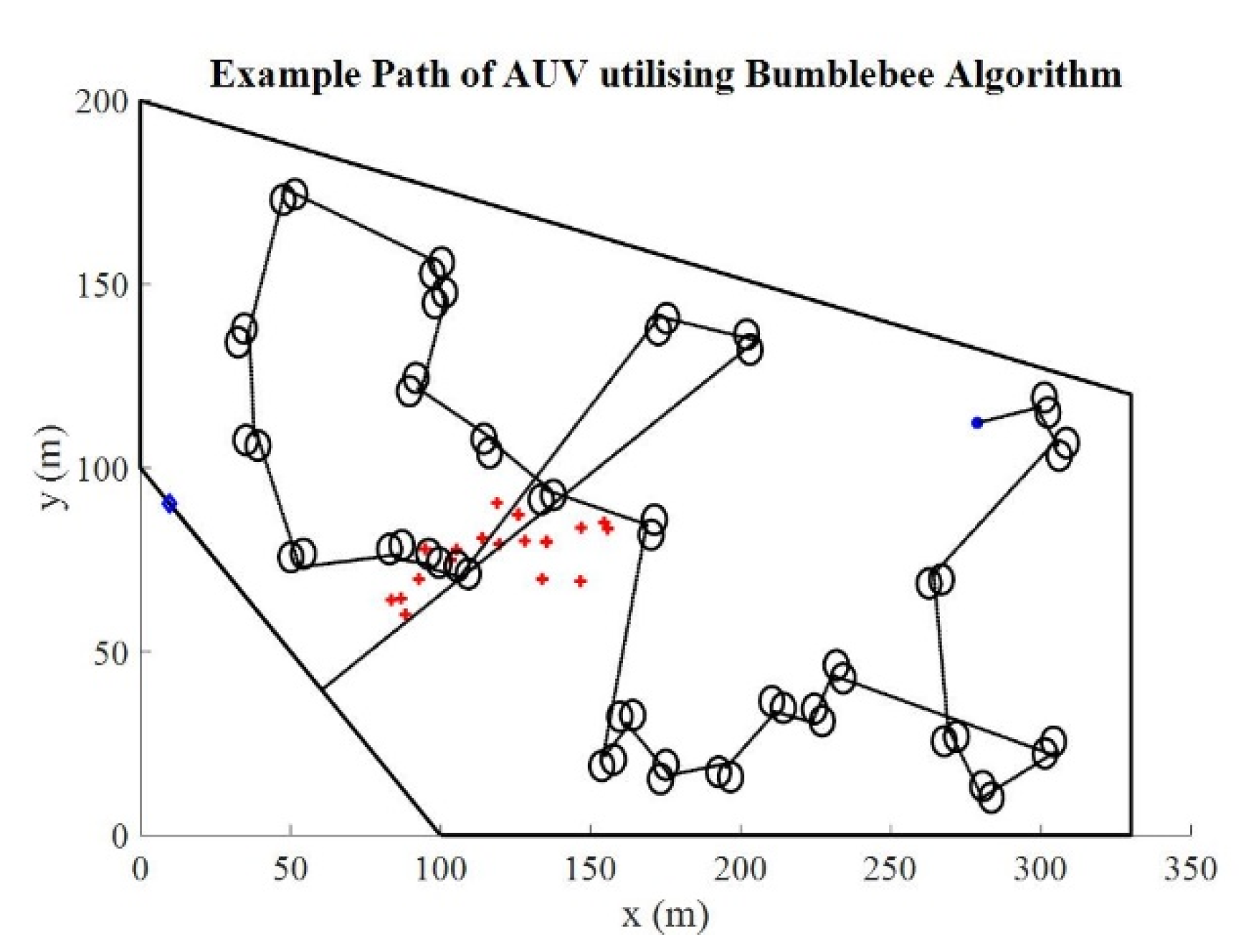
Figure 17 shows an example trajectory of a single AUV utilising the BB algorithm as the search strategy. It can be observed that the generated waypoints are spread over the whole search area, allowing the exploration of the entire area under investigation. However, it can further be seen that the search strategy does not exploit the information gained during the search for an adaption of the search path to exploit promising regions in more detail.

All search strategies, except the pre-defined strategy, require a randomised starting point for each AUV. However, in the real world, the system would be operated from a jetty or from a moored boat. In both cases, all AUVs start from the same fixed position somewhere within the search area. Therefore, in this study, prior the start of the search, a random start position is chosen for each AUV. To save energy, the vehicle travels from the jetty to the selected starting point surfaced. Therefore, only 80 percent of the travelled distance is counted for the travel distance of the AUV. An overview of all search strategies, including the number of tuneable parameters and the chosen start points of the AUVs is presented in

Table 1. Summarised search strategies for submarine groundwater discharge (SGD) investigation.

#	Search Strategy	Number of Parameters	Start Positions
1	Pre-defined path planning	none	Defined positions in edges
2	Adopted random walk	none	Random position
3	Particle Swarm Optimisation	4	Random position
4	Inertia Levy-flight	1	Random position
5	Self-Organising Migrating Algorithm	2	Random position
6	Bumblebee	2	Random position

.

4. Experiments (Simulations)

Different search strategies for a small swarm of AUVs are presented above. To allow a comparison between the search strategies, different computer simulations were executed. In the first step, a parameter study was undertaken to investigate the influence of the control parameters on the different search strategies. Subsequently, the influence of communication errors, localisation errors, and limited travel distance on the performance was investigated. During these experiments, the whole swarm, which consisted of three AUVs, explored the search space using the same search strategy. In another set of experiments, each AUV was allowed to select a different search strategy and the performance of this static combination of search strategies was evaluated. In the last set of experiments, the performance of a dynamic search strategy selection approach utilising a Fuzzy Logic system was examined.

For each experiment, a start time was chosen randomly between three hours before and three hours after low tide. As mentioned above, the maximum SGD inflow was expected to be during low tide. However, other constrains, such as survey during daytime or permissions from the authorities might require the surveys to take place at other times around low tide. The starting time window is depicted in Figure 7.

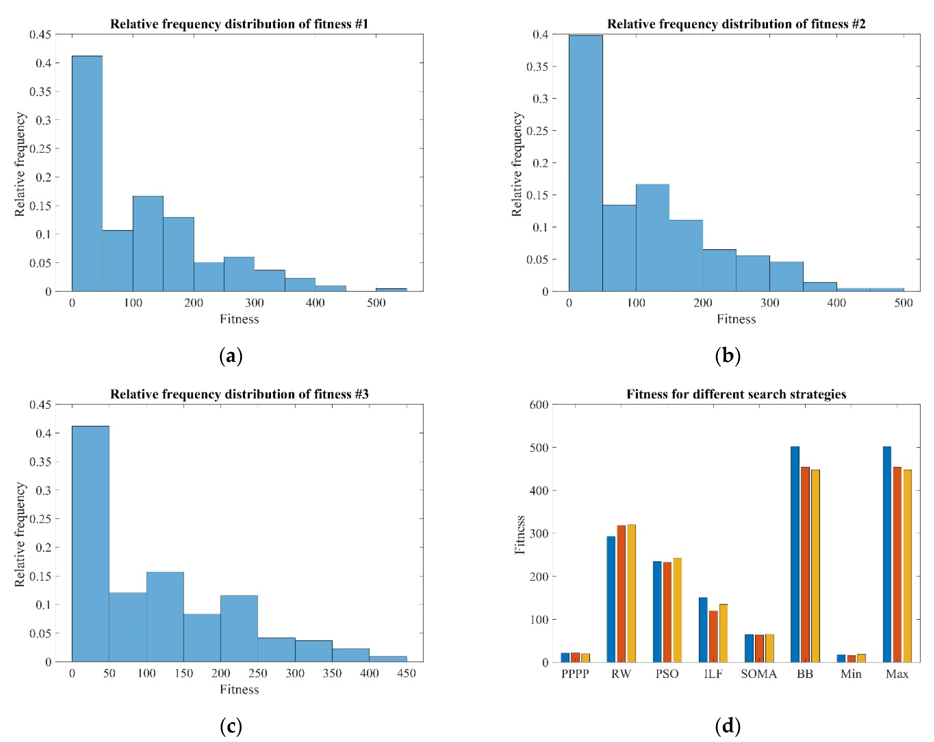
A measure for success of a search strategy is needed for the best strategy selection. This measure should reflect which search strategy best fulfils the intended aims of the search. In this study, the environment contained n SGDs with different flowrates. In the best case, the search strategy would be able to guide the swarm of AUVs to visit all the SGDs within the given maximum travel path lengths. Hence, the minimum distance between all members of the AUV swarm and all the SGDs is used for fitness evaluation. In addition, the flowrate of the different SGDs should be taken into account. This means it is more important to investigate SGDs with higher inflow, rather than visiting SGDs with lower inflow. Therefore, the performance of a search run is calculated as follows:

$$E=\frac{1}{n}{\displaystyle \sum }_{i=1}^n\frac{1}{\beta }·\underset{}{\min }\left(d_{1:t,i}\right).$$

(23)

where $E$ represents the performance of the search run, $n$ denotes the number of SGDs in the environment, $\beta$ represents the flowrate coefficient according to Equation (1), and $d_{1:t,i}$ denotes the distances between all the AUVs and the SGD i for all time steps {1…t}. However, applying single objective optimisation algorithms requires a scalar fitness value. Therefore, the performance over all search runs needs to be further condensed. For instance, the average performance over all runs could be used to assess the performance of a particular search strategy. In addition, a search strategy that performs better in some search runs should be rewarded. Thus, the following fitness measure was used in this research:

$$F=\underset{}{\min }\left(E\right)+2·\overline{E}.$$

(24)

where $F$ denotes the fitness value used for performance measure and optimisation, $E$ denotes the error values of all runs calculated according to Equation (23), and $\overline{E}$ represents the mean value of $E$.

4.1. Influence of Control Parameter Variation

Some of the proposed search strategies are based on stochastic optimisation algorithms. These algorithms usually feature a certain number of control parameters (Table 1). Recent research revealed the performance dependency of such optimisations algorithms on the right choice of control parameter values [24]. However, the right values of the control parameters usually depend on the optimisation problem at hand. Hence, in the first set of experiments, the influence of control parameters on the search performance of the different search strategies was investigated. For all the simulations, the distance-based localisation model (Equation (10)) with a basic standard deviation ${\sigma }_0=1 m$ and a distance-based standard deviation of $\sigma \left(d\right)=0.02 m/m$ was used. The values are based on the accuracy of the short baseline localisation system (SBL) used during the ROV surveys [83]. Within the simulations, the communication between the AUVs was error-affected, using the model described above. The damping coefficient was set to $\alpha =2$, while the normalising distance parameter was set to $d_0=100 m$. The maximum travel distance of the AUVs was set to 2700 m. These settings are based on the actual AUV platform used.

The PSO algorithm includes three different control parameters [84], the cognitive learning factor c₁, the social learning factor c₂, and the inertia factor $\omega$. However, in this implementation, the time constant $\Delta t$ is added as additional control parameter [70]. Within these experiments, all possible permutations of the four control parameters were evaluated using the following values:

$$\begin{gathered} c_1=\left\{0, 0.5, 1.0, 1.5, 2.0, 2.5\right\}, \\ {c}_2=\left\{0, 0.5, 1.0, 1.5, 2.0, 2.5\right\}, \\ \omega =\left\{0.1, 0.5, 1.0, 1.5, 2.0, 2.5\right\}, \\ \Delta t=\left\{1, 5, 10\right\} \mathrm{s}. \end{gathered}$$

(25)

ILF was developed to decrease the number of control parameters [76]. For this algorithm, only one control parameter, i.e., the maximum step length S needs to be tuned. For the experiments, the maximum travel distance was varied as follows:

$$S=\left\{1, 5, 10, 20, 50, 75, 100, 150, 200, 400, 600, 1000\right\} \mathrm{m}.$$

(26)

The SOMA algorithm includes three control parameters [77], the size of the jumping step $t$, the perturbation probability $p_{prt}$, and the maximal random integer $i_{max}$. During the parameter study, these parameters were varied as follows:

$$\begin{gathered} t=\left\{0.1, 0.25, 0.5, 1.0, 5.0, 10.0\right\}, \\ {p}_{prt}=\left\{0, 0.1, 0.2, 0.5, 0.75, 0.9, 1.0\right\}, \\ {i}_{max}=\left\{1, 2, 3, 5, 10\right\}. \end{gathered}$$

(27)

The BB includes two control parameters [52], the radius of the loops $r_{Loop}$ and the distance between the loops $d_{Loop}$. This distance $d_{Loop}$ was implemented as a multiplier of the radius of the loops $r_{Loop}$. Within the parameter study, both parameters were varied as follows:

$$\begin{gathered} t=\left\{0.1, 0.25, 0.5, 1.0, 5.0, 10.0\right\}, \\ {p}_{prt}=\left\{0, 0.1, 0.2, 0.5, 0.75, 0.9, 1.0\right\}, \\ {i}_{max}=\left\{1, 2, 3, 5, 10\right\}. \end{gathered}$$

(28)

The results of the experiments are presented in the results section of this paper. The optimal control parameter settings, found during the parameter study, were used for the subsequent experiments.

4.2. Influence of Localisation and Communication Error

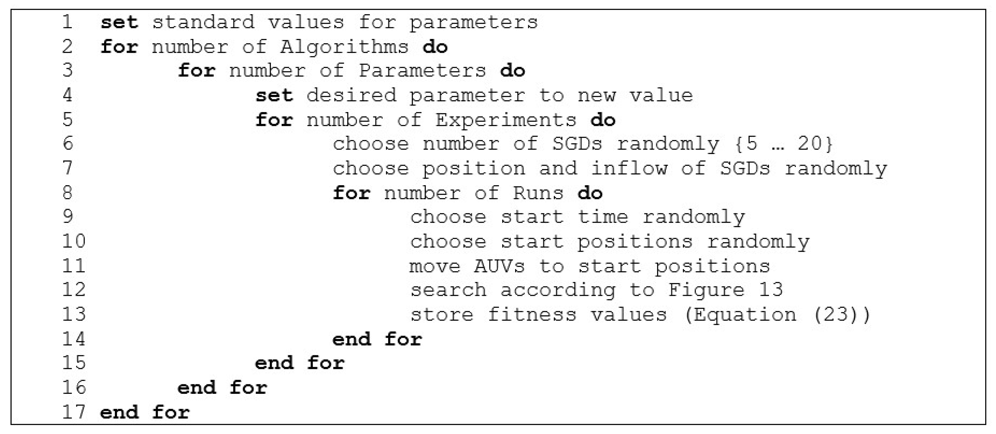
Previous published research indicates an influence of localisation and communication errors on the performance of different search algorithms [65]. Therefore, the influence of both errors on the performance of the search strategies was investigated in this study. Both errors were studied independently, utilising the aforementioned error models. The distance independent localisation error model was used. All the algorithms were tested with different parameter values for the standard deviation of the localisation and the damping coefficient. For each value, 10 different environment settings with randomly selected numbers and positions of SGDs were tested. For each setting, 10 search runs were carried out. For each run, the start time and the start positions of the AUVs were selected randomly as described above. The performance of each run (Equation (23)) was stored for analysis. The described procedure is summarised in the pseudocode presented in Figure 18.

4.3. Influence of Maximal Travel Distance

The maximum distance an AUV can travel depends on the energy stored on the vehicle, the energy consumption for propulsion, and environmental effects, such as currents. It was shown in recent research that the maximum distance an AUV can travel has an influence on the success of a search [85]. Hence, the influence of travel distance limitations on the proposed search strategies was examined. In the experiments, communication and self-localisation errors were modelled using the same parameters as for the control parameter study. For the experiments, the maximum travel distance l_max for each AUV was varied between:

$$l_{max}=\left\{500,600,\dots ,2600,3500\right\} \mathrm{m}.$$

(29)

For each l_max, 100 runs were carried out, following the procedure described in Figure 18.

4.4. Combined Search Strategy

In general, in most search strategies, exploration and exploitation capabilities need to be balanced to achieve good results [86,87]. However, the balancing of exploration and exploitation of a single algorithm can be a challenge [88]. Hence, a combination of different search strategies potentially accelerates the overall performance of a swarm. In a previous study, different algorithms were combined within a hyper heuristic to guide the AUVs’ search [78]. In this study, the algorithms are used independently. However, potentially utilising different search strategies on each AUV can accelerate the search performance. During the search, all the AUVs shared their best-known position regardless of the chosen strategy. For comparison, all possible combinations of different search algorithms were tested. To evaluate the performance, 100 runs were conducted for each combination, following the procedure described in Figure 18. During the experiments, communication and self-localisation error was modelled using the same parameters as for the control parameter study. The experiments were repeated three times.

4.5. Dynamic Search Strategy Selection

Another possible approach could be to select a suitable search strategy dynamically, based on the current status of the search. This dynamic selection can be viewed as BBP [8]. However, switching between different search strategies usually requires the definition of thresholds to control the switching processes [89]. The correct determination of thresholds can influence the search behaviour of the system.

In this study, a fuzzy logic approach [27] was utilised for dynamic search strategy selection. MFs and rules were implemented as Mamdani fuzzy inference system [90] utilising the “Fuzzy Logic Designer” from MATLAB’s Fuzzy Logic Toolbox [91]. This toolbox was used to develop fuzzy logic systems in recent research [29,34]. Obtaining estimations from the fuzzy logic inference system (FIS) requires defuzzification [92]. Here, the centroid defuzzification scheme was used.

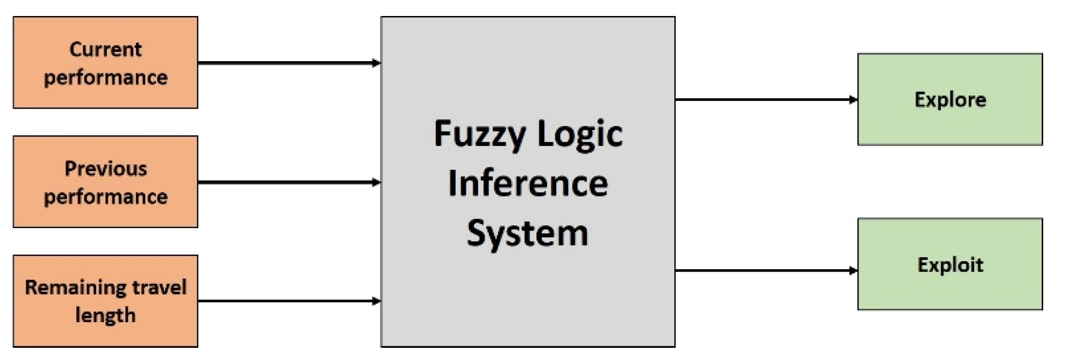
The dynamic selection is based on the current and the previous progress of the search. In addition, the remaining energy, available for travelling, is taken into account. Therefore, three inputs, current performance, previous performance, and remaining travel distance, were defined. The current performance indicator is calculated as follows:

$$g_{p,i}=\frac{p_i-g_w}{g_b-g_w}.$$

(30)

where $g_{p,i}$ denotes the performance indicator for the current time step, p_i denotes the current fitness, g_w represents the worst fitness found so far by the entire swarm, and g_b is the best fitness found so far by the entire swarm. For the previous performance indicator, the AUV stores the fitness every time it reaches a waypoint. The previous performance indicator is then calculated as follows:

$$g_{p,i-1}=\frac{p_{i-1}-g_w}{g_b-g_w}.$$

(31)

where $g_{p,i-1}$ denotes the performance indicator for the previous waypoint. The remaining travel distance indicator is calculated as follows:

$$t_{p,i}=\frac{l_i}{l_0}.$$

(32)

where $t_{p,i}$ represents the travel distance indicator, $l_i$ denotes the currently remaining travel distance, and $l_0$ represents the maximal travel distance of the AUV. These indicators are calculated every time an AUV reaches a waypoint. Subsequently, these values are fed into the FIS. The FIS than calculates the values for the two outputs, i.e., explore and exploit (Figure 19). The calculation of the outputs is based on the defined MFs and the rule base system.

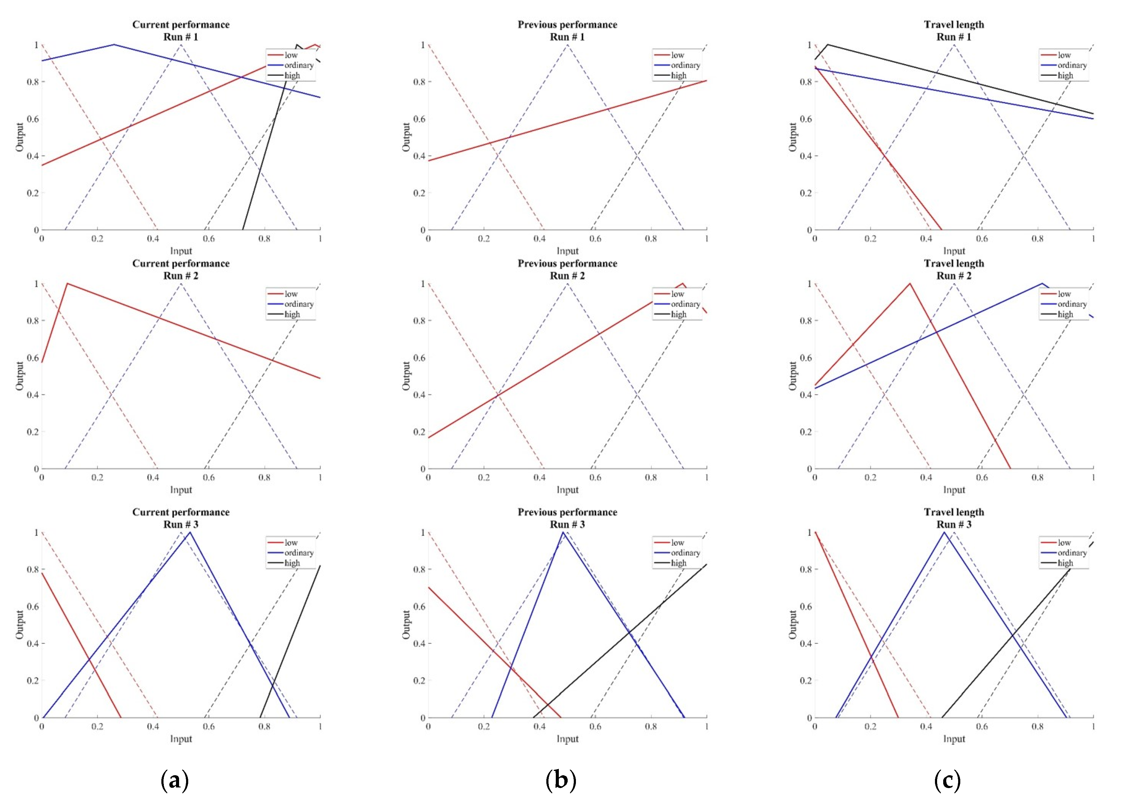
The utilisation of fuzzy logic requires the definition of MFs for any inputs and outputs of the fuzzy system. The MFs are used for the fuzzyfication of the inputs and the defuzzizication of the outputs. The number, shape, and location of the different MFs usually have an important impact on the performance of the FIS. However, the determination of the MFs requires some knowledge about the problem at hand, and, in addition, fine tuning of the parameters to optimise the performance of the FIS. Three MFs, named low, ordinary, and high, were defined for each input and each output. They were defined as triangle MFs. The low MFs start with an output of 1 at an input value of 0 and decreasing to an output value of 0 for the input value of 0.417. The ordinary MFs start with an output of 0 for the input of 0.083, increasing to a maximum output of 1 for the input of 0.5. For higher inputs, the output decreases until the output is 0 again for inputs of 0.917. The high MFs also start with an output value of 0 for an input value of 0.584. The output increases to the maximum value of 1 for the input value of 1. The shapes of the MFs are shown in the results section figure.

Rules in fuzzy logic are based on the knowledge of experts in the field to which fuzzy logic is applied [29]. In a FIS, the rule base is given as a set of if-then statements [29,92]. Here, the desired behaviour of an AUV during the search was used to tailor the rule base of the FIS. If the current performance of the AUV is good, exploiting the area near the current position might lead to finding better positions. However, if the current performance of the AUV is poor, it might be more effective to explore other areas to find better places away from the current position of the AUV. In addition, the remaining energy of the AUV plays an important role. If the remaining energy is high, the AUV can potentially explore other areas even if the current performance is average. However, if the remaining energy of the AUV is low, it should avoid travelling longer distances to save energy. The aforementioned expected search behaviour was used to formulate the rule base system of the FIS. All the rules used in this research are summarised in

Table 2. Rule base of the fuzzy logic inference system (FIS) used for dynamic search strategy selection.

#	Input			Output
	Current Performance	Previous Performance	Travel Distance	Explore	Exploit
1	none	none	low	low	high
2	low	low	high	high	low
3	low	low	ordinary	high	low
4	low	low	low	high	low
5	low	ordinary	high	high	low
6	low	ordinary	ordinary	high	ordinary
7	low	high	none	low	high
8	ordinary	ordinary	high	high	low
9	ordinary	ordinary	ordinary	ordinary	ordinary
10	ordinary	ordinary	low	low	high
11	ordinary	high	none	low	high
12	high	none	none	low	high
13	ordinary	low	none	ordinary	high

.

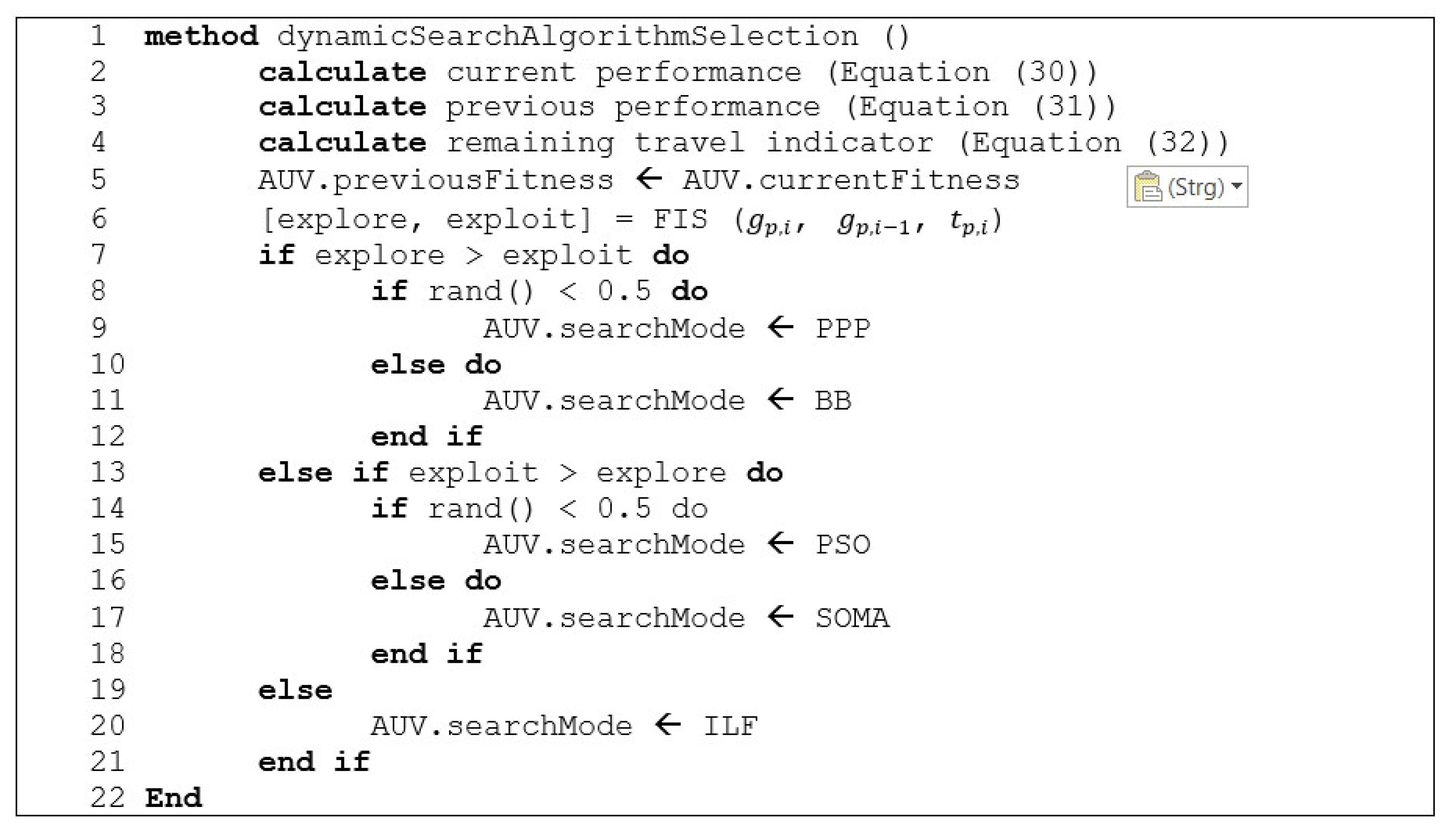
Based on the outputs of the FIS, an appropriate search strategy is chosen by the AUV. Therefore, the search strategies were divided into exploring and exploiting algorithms. PPP and BB were classified as exploring algorithms, while PSO and SOMA were defined as exploiting algorithms. ILF was used as fall-back algorithm for the case of equality between exploring and exploiting output of the FIS. RW was not used for the dynamic selection approach. The selection from the group of suitable algorithms was undertaken randomly. The procedure of dynamic selection of a suitable search strategy, described above, is summarised as pseudocode in Figure 20.

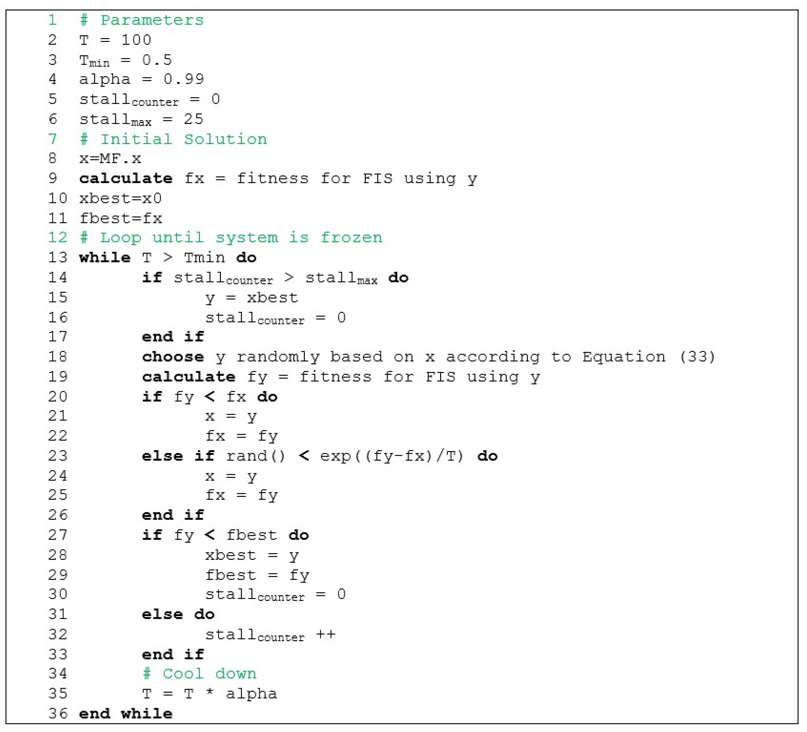
The FIS was built on expert knowledge and the expected behaviour of the AUV during the search. The MFs of the different inputs and outputs were designed as regular triangle functions covering the whole input space. However, it cannot be guaranteed that these triangular shapes best solve the problem at hand. Therefore, the shapes of the input MFs were optimised utilising Simulated Annealing (SA) [93]. For each input, three triangle-shaped MFs were defined. Each MF contained three parameters A_n, B_n, and C_n. The value of the parameters can be chosen according to:

$$\left\{A_n,B_n,C_n\in ℝ | A_n\le B_n\le C_n\right\}.$$

(33)

The total number of optimisation parameters is 27. The MFs defined above were chosen as starting point for the optimisation. In each iteration of the optimisation process, a new set of parameters was selected and evaluated. For this evaluation, the selected values were used to define the shapes of the MFs of the inputs. Utilising these MFs, 100 search runs, as described in Figure 13 were conducted, and the fitness (Equation (24)) was calculated. The optimisation process is summarised as pseudocode in Figure 21. The whole optimisation process of the MFs was repeated three times.

5. Results

In the previous section, several experiments were described, focusing on different aspects of the search capabilities of a small swarm of AUVs. Hereafter, the results of the different experiments are presented.

5.1. Influence of Control Parameter Variation

The influence of the control parameters on the performance of the different search algorithms was investigated. However, PPP and RW do not utilise any control parameters. Meanwhile, for comparison, the performances of PPP and RW were also investigated. For both strategies, five sets of experiments were conducted. The average fitness was 20.4 for PPP and 295.4 for RW. The final fitness of all runs are summarised in

Table 3. Fitness of pre-defined path planning (PPP) and adopted random walk (RW).

Strategy	Run 1	Run 2	Run 3	Run 4	Run 5	Average
PPP	18.9	20.6	19.0	18.2	25.3	20.4
RW	291.4	300.4	266.8	281.3	337.2	295.4

.

The results of the control parameter study are provided in Figure 22. The results for all the parameter combinations are summarised in histograms for PSO, SOMA, and BB. For ILF, the results are given as a line chart over the maximum step length.

Utilising the PSO search strategy, the best fitness value found was 177.6. This fitness was obtained with the cognitive scaling factor set to $c_1=0$, the social scaling factor set to $c_2=0.5$, the inertia set to $\omega =1.5$, and the time step set to $\Delta t=10$. The best fitness value found by ILF was 118.1. This value was achieved with a maximum step length $S=600 m$. The best-performing algorithm was SOMA, with a minimum fitness value of 47.1. This fitness was achieved for jumping step size $t=1$, perturbation probability $p_{prt}=0.1$, and maximum integer $i_{max}=10$. The best fitness value found by BB was 309.5, which was the worst across all six algorithms under investigation. This performance was achieved with loop radius $r_{loop}=6 m$ and loop offset multiplier $d_{loop}=0.5$.

From the different plots in Figure 22, it can be observed that the chosen control parameters have a significant influence on the performance of the search. In the further experiments of this study, the control parameters were set to the best values identified in this parameter study.

5.2. Influence of Localisation and Communication Error and Maximum Travel Distance

The median of the error of the different search strategies (Equation (23)), including the standard error of the mean as error bars, over an increasing standard deviation $\sigma$ of the distance-independent localisation model (Equation (9)), are shown in Figure 23a. It can be observed that all the algorithms, except for BB, seemed to be unaffected by localisation errors. For a standard deviation error $\sigma \le 2,$ the median error of BB was in the same order of magnitude as the error of the other algorithms. However, for $\sigma >2$, the median error of BB increased. The median error of PPP and SOMA show a similar shape for the all tested standard deviations. The best performance was achieved by PPP and SOMA, followed by ILF, PSO, and RW.

The median of the error of different search strategies (Equation (23)), including the standard error of the mean as error bars, over the increasing damping coefficient $\alpha$ of the communication error model (Equation (11)), are shown in Figure 24a. It can be observed that all the algorithms, except for PSO and SOMA, were unaffected by disturbed communication. For damping coefficients $\alpha \ge 2$ the performance of SOMA was in the same order of magnitude as PPP. The best performance was shown by PPP, followed by BB, SOMA, ILF, PSO, and RW.

Figure 25 shows a comparison between the different search strategies for varying maximum travel distance. All the algorithms, except for PSO, were influenced by shorter maximum travel distance by the AUVs. The performance of PPP increased with increasing maximum travel distance. However, for maximum travel distances > 1800 m, the median error appeared constant. The influence of shorter travel distance on ILF and RW was in the same order of magnitude. However, the performance of ILF was better than the performance of RW. The effect of shorter travel distances on SOMA was smaller than on PPP or ILF. For maximum travel distances < 1200 m, SOMA outperformed all other strategies. In addition, it can be observed that only BB showed better performances for shorter travel distances than for longer distances.

In Figure 23b, Figure 24b, and Figure 25b the fitness, calculated following Equation (24), is shown for the localisation error, the communication error and the maximum travel distance respectively. The figures are included to allow a comparison with other experiments conducted. In addition, the maximum deviation of the mean errors for the different search algorithms and the three different experimental setups are summarised in

Table 4. Summarised maximum deviations of the mean error values for the six search strategies and the localisation error, communication error, and the maximum travel distance surveys.

	Range of Mean Error
Strategy	Localisation Error	Communication Error	Maximum Travel Distance
PPP	13.7	1.2	164.3
RW	39.3	38.5	92.0
PSO	53.5	74.0	44.6
ILF	34.9	12.7	115.8
SOMA	32.8	29.1	63.9
BB	329.9	5.2	137.3

.

5.3. Combined Search Strategy

The performances of all the possible combinations of the search strategies were evaluated. The experiments were repeated three times. Histograms of the scored fitness of the different runs are shown in Figure 26a–c. The minimum fitness of the three repetitions was 17.9, 15.9, and 18.9, respectively. The maximum fitness values of the three repetitions were 502.4, 453.9, and 447.6. Also, 41.2%, 39.8%, and 41.2% of the runs scored a fitness $F\le 50$. In all of these runs, at least one AUV used the PPP search strategy.

In addition, the performance of the runs, where all AUVs follow the same search strategy, together with the best and the worst combination, are shown in Figure 26d. It can be seen that, for a swarm with a single search strategy, PPP performed best, scoring fitness values of 21.3, 22.4, and 19.5 for the three repetitions, respectively. The second best performance was shown by SOMA, with fitness values 64.5, 63.5, and 65.7 for the different runs. It can be observed from Figure 26d that the performance of BB was the worst out of all the combinations. The compositions of the swarm with the best performances from all three repetitions are summarised in

Table 5. Overview of the best combined search strategies from the three repetitions.

Repetition	AUV 1	AUV 2	AUV 3	Fitness
1	PPP	SOMA	PSO	17.9
2	PSO	PPP	PPP	15.9
3	SOMA	PPP	PPP	18.9

.

5.4. Dynamic Search Strategy Selection

The MFs for the different inputs were optimised utilising SA. The optimisation process was repeated three times; all the optimisations started with initial MFs described above. The development of fitness over time is shown in Figure 27 for the three runs. It can be observed that in all three optimisation runs, SA was able to increase the performance of the search by adjusting the MFs used for dynamic search strategy selection. The order of best performance of the three optimisation runs was f_best,R1 = 19.1, f_best,R2 = 18.2, and f_best,R3 = 19.5 respectively.

Each MF was implemented as triangle MF, requiring three parameters. The optimiser was allowed to adjust the parameter values of the three MFs of the three inputs. Therefore, a total number of 27 parameters was optimised. The optimised MFs for the three input variables are shown in Figure 28. It can be observed that the best solutions of the different runs are based on different shapes of MF.

The performance of the dynamic selection approach, utilising the optimised MFs, was further investigated. For each set of MFs, 100 additional runs were carried out. During the runs, the time, the AUVs following the different search strategies, together with the scored performance, were logged. The fitness of the different runs is summarised as boxplot (Figure 29a), while the time spent on different search strategies is shown in Figure 29b. It can be seen that MFs from run 1 and run 2 presented a better performance than the non-optimised MFs and the MFs from run 3. The mean fitness of the 100 runs were 28.7, 21.7, 22.7, and 26.9 for the non-optimised MFs and the three sets of optimised MFs, respectively. The minimum fitness was 22.6, 17.6, 17.3, and 20.9, while the maximum fitness was 35.0, 26.1, 29.3, and 36.7 for the four different sets of MFs, respectively. It can be observed that for all four sets of MFs, the swarm only spent about 1% of the search time utilising the PSO. For all MFs, except run 2, the swarm spent most of the search time using PPP, i.e., 55%, 43%, and 41% for the non-optimised and the optimised MFs from run 1 and run 3, respectively.

6. Discussion

6.1. Parameter Study

The results from the parameter study, shown in Figure 22, revealed a strong influence of the parameter settings on the performance of the different search strategies. The best parameter settings, found for PSO, are similar to the best settings found in previous research for a similar problem [24]. However, utilising these settings, the cognitive knowledge of the single AUVs was not utilised during the search. In this case, Equations (15) and (16) can be simplified to:

$$p_{i+1}=p_i+\left(g_{best}-p_i\right)·c_2·r_2·\Delta t+v_i·\omega ·\Delta t.$$

(34)

This simplified equation of PSO shows some similarities to the SOMA update rule given in Equation (21). However, the best fitness, demonstrated by SOMA, was 47.1, while the best fitness, demonstrated by PSO, was 177.6. The main difference between Equations (21) and (34) is the last summand of Equation (34), were the current velocity of the agent is used. However, this velocity is affected by all the decisions an agent has already made during recent search steps. Hence, due to the inertia of the algorithm, the AUV is not able to change its direction as quickly as SOMA to react to changes in the environment.

During the parameter study, the best fitness scored by BB was in the same order of magnitude as the performance of RW. BB does not utilise any feedback information, gained during the search, to guide the agent towards promising regions. Therefore, BB can be understood as random walk with an additional local search component.

For ILF, only a single control parameter, the maximum step size S, was optimised during the parameter study. As shown in Figure 22b, the performance of ILF increased with increasing values of the parameter S. However, for values of S > 150, the influence on the performance can be neglected. From Equations (17)–(19) it can be observed that small values of S limit the exploration capabilities of ILF. Hence, the agent is not able to explore other parts of the area under investigation. For values S > 600, a slight decrease in the fitness was obtained. This might have been caused by the shape and size of the search area. If the agent is able to choose steps bigger than the dimensions of the search area, the agents are likely to travel from one border of the search area to the other, wasting large amounts of the AUV’s energy.

6.2. Influence of Localisation and Communication Errors and Maximum Travel Distance

As shown in Figure 23, all the search strategies, except for BB, were unaffected by localisation errors. The strong influence of localisation errors on the performance of BB can be explained based on the chosen implementation of the algorithm. For BB, all the waypoints were generated prior the search based on the maximum travel distance (Figure 16). During the waypoint generation, the travelled distances were calculated based on the shortest distance between the waypoints. During the search, the nearest randomly generated waypoint was selected as the destination. In each iteration, the AUV calculated the heading for the next step based on its own estimated position and the position of the destination. Localisation uncertainties resulted in zigzag movements of the AUV while approaching the destination. Due to the zigzag movements, the AUV required more energy than expected to reach the waypoints. Therefore, the AUV could not visit all the waypoints planned prior to the search. Hence, some parts of the search area were not explored, leading to the poor performance of BB.

For PPP, a slight decrease in the performance can be observed for large standard deviations of the localisation error $\sigma >8 \mathrm{m}$ (Figure 23b). PPP also utilises a list of waypoints generated prior the search. However, the number of waypoints used by PPP was smaller than the number of waypoints used by BB. In addition, PPP used fixed starting points for the AUVs, located in different edges of the search area. This extended the area covered, even if the whole list of generated waypoints was not visited. PSO and SOMA were not influenced by increasing localisation errors. The performance of RW and ILF were not influenced by localisation or communication errors.

Only PSO and SOMA utilised information gained from other agents during the search. Hence, only these two algorithms should be influenced by a disturbed communication between the AUVs. As shown in Figure 24 and summarised in Table 4, the performance of PSO was much more affected by large communication errors than SOMA. As given in Equations (15) and (21), both strategies utilise the knowledge of the swarm in a similar way. Therefore, the performance differences may have been caused by the control parameter values or the additional term of PSO utilising the past decisions of the AUV.

As expected, the performance of PPP was highly influenced by shorter travel distances of the AUVs. However, for travel distances greater than 1800 m, the influence on the performance can be neglected. The influence of the maximum travel distance on the performance of SOMA was low, with a derivation of the mean errors of 63.9. In addition, for maximum travel distances lower than 1700 m, the performance of SOMA was better than the performance of PPP.

The performance of PSO was unaffected by shorter travel distances of the AUVs, resulting in the lowest deviation of the mean errors of all the search strategies investigated (Table 4). However, the general performance of PSO was worse compared to some of the other algorithms, such as SOMA. As expected, both RW and ILF showed an improvement in performance with increasing maximum travel distance.

Against our expectations, the BB search showed a comparably good performance for very short maximum travel distances. The best performance of BB was found for the maximum travel distance of 600 m, while the performance decreased with increasing maximum travel distances. For maximum travel distances greater than 900 m, the performance of BB seemed to be unaffected. The good performance of BB for very limited travel distance only can be explained by the waypoint generation drawn in Figure 16. The waypoints are generated randomly within the whole search area. For longer maximum travel distances, the density of points increases. However, as described above, due to localisation errors, not all waypoints were visited. With fewer generated waypoints, the probability of visiting other regions of the search space is potentially higher.

With unlimited energy, stored on the AUVs, PPP would be the best search strategy, because it is the only strategy that can guarantee the full coverage of the entire area under investigation. However, with limited energy capacity, cooperative search strategies, such as SOMA, can outperform PPP.

6.3. Combined Search Strategy

The experiments for the combined search strategies were repeated three times. As shown in Figure 26a–c, the three repetitions showed similar results. Therefore, the limited set of 100 experiments, as described in Figure 13, is applicable to answering questions about the quality of different search strategies. It can be seen from Table 5 that a combination of the exploration capabilities of PPP and the exploitation capabilities of PSO and SOMA can increase the overall performance of the swarm. The overall best performance was achieved for the combination of two AUVs following PPP and one AUV utilising PSO. However, it cannot be seen from Table 5 whether a combination of search strategies clearly outperforms all other combinations. Therefore, the best ten combinations of the three repetitions are summarised in

Table 6. Best ten combinations of the three repetitions; the search strategies are coded as follows: 1: pre-defined path planning (PPP), 3: particle swarm optimisation (PSO), and 5: self-organising migrating algorithm (SOMA).

#	Run 1				Run 2				Run 3
	A 1	A 2	A 3	F	A 1	A 2	A 3	F	A 1	A 2	A 3	F
1	1	5	3	17.9	3	1	1	15.9	5	1	1	18.9
2	1	3	1	19.5	1	5	3	17.6	1	1	3	19.0
3	1	1	3	19.8	1	3	5	18.7	1	1	1	19.5
4	3	1	1	20.0	1	3	1	18.7	1	3	3	20.4
5	3	1	5	20.0	3	1	5	20.0	1	3	5	20.8
6	1	3	5	21.3	1	1	3	20.4	3	1	1	21.3
7	1	1	1	21.3	1	5	5	21.1	1	5	5	21.5
8	3	5	1	21.7	5	1	5	21.1	5	1	3	21.7
9	5	1	1	21.8	5	1	1	22.0	1	3	1	21.8
10	1	5	1	21.8	5	1	3	22.3	1	5	3	21.9

. In all cases, at least one AUV utilised the PPP algorithm, while, in most cases, at least one AUV utilised PSO or SOMA. From the total number of 30 combinations, 20 utilised PSO, while 17 utilised SOMA. Just two combinations utilised only PPP. Interestingly, the participation of PSO yielded very good results.

The experiments showed that RW, ILF, and BB are not able to improve the performance of the swarm. The average fitness of the best combinations of search strategies is 16.6% better than the average performance of the swarm using only PPP for all three AUVs.

6.4. Dynamic Search Strategy Selection

Simulated annealing (SA) was able to improve the performance of the dynamic search strategy in all three optimisation runs (Figure 27). The performance of the optimised dynamic search strategy selection was in the same order of magnitude as the best performance of the combined search strategies, discussed above. However, as shown in Figure 27, over long periods of iterations, SA was not able to find better solutions. Therefore, other parameter settings of SA or other optimisation strategies, such as the genetic algorithm [94], can potentially improve the optimisation results.

The maximum fitness difference between the three optimisation runs was 1.3. However, as shown in Figure 28, the shapes of the optimised MFs are different for all three solutions. For the first and second solution, the optimiser did not keep all the MFs. As an example, for MFs from optimisation run 1 and run 2, the input previous fitness indicator only kept a single MF, the low MF, after the optimisation. If an MF does not cover the input space, the output from this MF will always be zero. Therefore, due to the reduced number of MFs, only a set of the rules, defined in Table 2, was applicable during the search when the optimised MFs were utilised. From Table 2 and Figure 28, it can be seen that the FIS, utilising the MFs from optimisation run 1, only use rules number 1, 2, 3, 4, 12, and 13. The FIS utilising the MF from optimisation run 2 makes use of rules 1, 3, and 4 only. However, optimisation run 3 simply amends the shapes of the MFs, while keeping all of them. Therefore, the FIS utilising MFs from optimisation run 3 uses all the rules defined in Table 2.

Utilising the MFs from optimisation run 2, the dynamic selection becomes a sequential search, first utilising the exploration algorithms PPP and BB and, after a certain period of time, switching to the exploitation algorithms PSO and SOMA. Figure 30 shows the development of the error and the utilised search strategies over the time of the search in a sample run. It can be observed that during the first part of the search, the AUVs switched between PPP and BB exploring the area under investigation. Subsequently, all the AUVs independently switched to exploitation algorithms.

From Figure 29b, it can be seen that the optimisation increased the time the swarm spent on exploitation. Furthermore, even if the shapes of the optimised MFs were not similar and the performance of the first run was much better than the performance from the third run (Figure 29a), one can observe similar swarm compositions for the MFs from the first and from the third optimisation run. Hence, it seems that not only the time spent on exploration and exploitation, but also the decision as to when to explore or exploit, played an important role in the performance of the search.

6.5. Comparison between Different Strategies

In this paper, different search strategies for AUVs were proposed. In addition, different strategies for an optimal swarm composition were evaluated. In this section, a comparison between the strategies for swarm composition is drawn. Therefore, the performances of the best combined search strategy and the best dynamic search strategy selection for different maximum travel distances are investigated and the results are compared to the results of the single search strategies presented in Figure 25. The results from this comparison are shown in Figure 31. In addition, the changes of error over time, for all runs and for each maximal travel distance, can be found as waterfall diagrams in Supplementary Material Figure S2. Furthermore, the paths of the AUVs for the best and the worst run for each maximal travel distance can be found in Supplementary Material Figure S3. It can be seen from Figure 31, that both the combined strategy and the dynamic search strategy selection are able to improve the search performance. For shorter maximum travel distances, the performance of the dynamic selection is equal the performance of SOMA. The performance of the combined search is worse than that of SOMA. However, both strategies outperform PPP for travel distances shorter than 1500 m. However, for longer maximum travel distances, both strategies demonstrate a similar performance to PPP and outperform both, SOMA and PSO.

The best possible search performance always leads to a fitness value of zero regardless the energy stored on the AUVs. Therefore, the performance of the different approaches can be measured by the area beneath the fitness curves given in Figure 31b, as follows:

$$A={{\displaystyle \int }}_{l_{min}}^{l_{max}}\overline{F}\left(l\right)dl.$$

(35)

where $l_{min}$ and $l_{max}$ denote the minimum and maximum values of the maximum travel distance respectively and $\overline{F}\left(l\right)$ represents the mean fitness scored for the corresponding maximum travel distance. The performance of the different strategies was A = 2.792 × 10⁵ for PPP, A = 7.361 × 10⁵ for PSO, A = 2.840 × 10⁵ for SOMA, A = 2.062 × 10⁵ for the combined strategy, and A = 1.875 × 10⁵ for the dynamic selection. Hence, it can be concluded that the dynamic selection strategy showed the best performance, followed by the combined strategy.

7. Conclusions

In this study, the performance of different search strategies applied for SGD detection were investigated using computer simulations. The dynamic simulation environment was built on in situ DO measurements and sonar backscatter data from a survey in Western Australia.

The influence of different factors, such as error-prone self-localisation or restricted communication, on the performance of the proposed algorithms was investigated. It was demonstrated that PPP outperformed all the other algorithms when all the AUVs used the same search strategy. On the other hand, with different search strategies for each AUV, the search performance of the whole swarm was improved by incorporating population-based search strategies, such as PSO and SOMA, within the PPP scheme. The best performance was achieved for the static combination of two AUVs following PPP, while the third AUV utilised PSO for the search. The performance of this combination was 26.4% better than that of PPP, based on the fitness-over-travel-distance variation.

In addition, a novel mechanism for the dynamic selection of search strategy was proposed and evaluated. This mechanism uses fuzzy logic and a set of defined rules to select the most suitable search algorithm. For different maximum travel distances of the AUVs, this dynamic approach was able to perform at least as well as the PPP and the SOMA strategies. However, due to its better adaptation to the current situation, the overall performance, calculated based on the fitness over travel distance curve, the proposed dynamic search strategy selection was 32.8% better than PPP and 34.0% better than SOMA.

The computer simulations showed that both the static combination and the dynamic search strategy selection scheme offer potential ways to utilise Artificial Intelligence optimisation algorithms such as PSO or SOMA as search strategies for AUVs.

In future research, both schemes will be evaluated further, using other search environments and practical field tests.