Coupled Engine-Propeller Selection Procedure to Minimize Fuel Consumption at a Specified Speed


Abstract
1. Introduction
2. Ship and Engine Specifications
3. Numerical Model
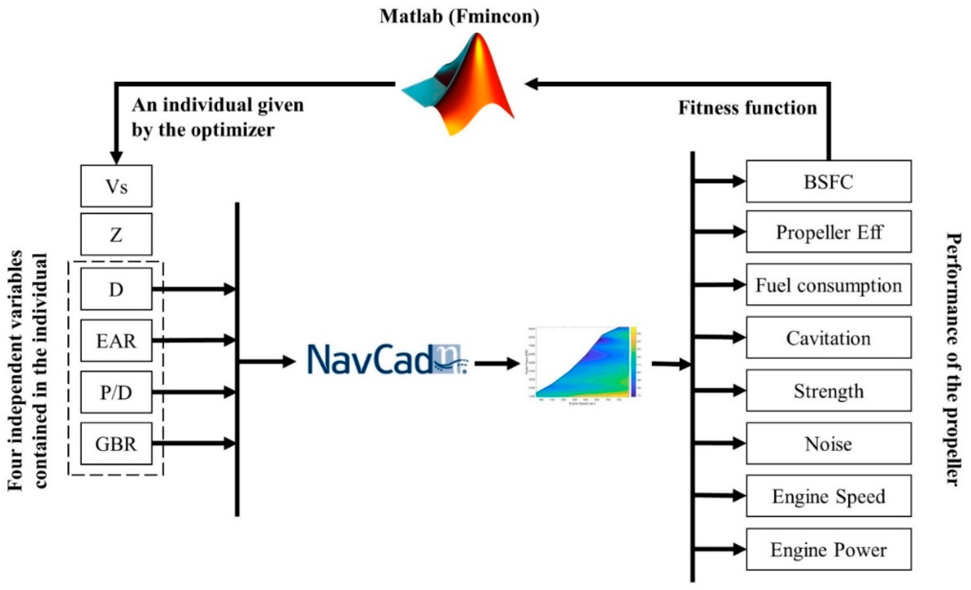
3.1. General Overview
3.2. NavCad Software
3.3. Engine Performance
3.4. Propeller Performance
4. Results and Discussion
5. Conclusions
Author Contributions
Funding
Institutional Review Board Statement
Informed Consent Statement
Data Availability Statement
Conflicts of Interest
Abbreviation List
| 1D | One-dimensional |
| BEM | Boundary elements method |
| BMEP | Brake mean effective pressure [bar] |
| BSFC | Brake specific fuel consumption [g/kW.h] |
| CFD | Computational fluid dynamics |
| Cn | Constant |
| CO2 | Carbon dioxide [g/kW.h] |
| D | Propeller diameter [m] |
| EAR | Expanded area ratio |
| FC | Fuel consumption [kg/nm] |
| FPP | Fixed pitch propeller |
| g(x) | static penalty function |
| GA | Genetic algorithm |
| GBR | Gearbox ratio |
| h | Propeller centreline immersion [m] |
| J | Advance coefficient |
| j | Number of constraints |
| k | Constant |
| KQ | Torque coefficient |
| KT | Thrust coefficient |
| MCR | Maximum continuous rate |
| MDO | Marine diesel oil |
| MOPSO | Multi-objective particle swarm optimization |
| n | Propeller speed [rps] |
| N | Propeller speed [rpm] |
| NOx | Nitrogen oxides [g/kW.h] |
| NSGA II | Non-dominated sorting genetic algorithm II |
| P/D | Pitch diameter ratio |
| Patm | Atmospheric pressure [Pa] |
| PD | Delivered power [W] |
| Pv | Vapour pressure [Pa] |
| Q | Torque [N] |
| Rn | Reynolds numbers |
| RT | Total ship resistance [N] |
| SC | Maximum allowable stress [N/m2] |
| Sn | Constant |
| SOx | Sulphur oxides [g/kW.h] |
| t | Thrust deduction factor |
| t | Blade thickness [m] |
| T | Thrust [N] |
| tn | Constant |
| un | Constant |
| VA | Advance speed [m/s] |
| vn | Constant |
| Vs | Vessel speed [m/s] |
| Vtip | Propeller tip speed [m/s] |
| w | Wake fraction |
| x | Number of optimization variables |
| Z | Propeller blades |
| γ | Specific weight [N/m3] |
| ηo | Propeller efficiency |
| ν | Kinematic viscosity [m2/s] |
| ρ | Density [kg/m3] |
References
- Lloyd’s Register. Implementing the Energy Efficiency Design Index; Lloyd’s Register: London, UK, 2012. [Google Scholar]
- Papanikolaou, A.; Zaraphonitis, G.; Boulougouris, E.; Langbecker, U.; Matho, S.; Sames, P. Multi-objective optimization of oil tanker design. J. Mar. Sci. Technol. 2010, 15, 359–373. [Google Scholar] [CrossRef]
- Prpić-Oršić, J.; Vettor, R.; Faltinsen, O.M.; Guedes Soares, C. The influence of route choice and operating conditions on fuel consumption and CO2 emission of ships. J. Mar. Sci. Technol. 2016, 21, 434–457. [Google Scholar] [CrossRef]
- Papanikolaou, A.; Zaraphonitis, G.; Bitner-Gregersen, E.; Shigunov, V.; Moctar, O.E.; Guedes Soares, C.; Reddy, D.N.; Sprenger, F. Energy Efficient Safe SHip Operation (SHOPERA). Transp. Res. Rec. 2016, 14, 820–829. [Google Scholar] [CrossRef]
- Vettor, R.; Tadros, M.; Ventura, M.; Guedes Soares, C. Route planning of a fishing vessel in coastal waters with fuel consumption restraint. In Maritime Technology and Engineering 3; Guedes Soares, C., Santos, T.A., Eds.; Taylor & Francis Group: London, UK, 2016; pp. 167–173. [Google Scholar]
- Vettor, R.; Tadros, M.; Ventura, M.; Guedes Soares, C. Influence of main engine control strategies on fuel consumption and emissions. In Progress in Maritime Technology and Engineering; Guedes Soares, C., Santos, T.A., Eds.; Taylor & Francis Group: London, UK, 2018; pp. 157–163. [Google Scholar]
- Jaurola, M.; Hedin, A.; Tikkanen, S.; Huhtala, K. Optimising design and power management in energy-efficient marine vessel power systems: A literature review. J. Mar. Eng. Technol. 2019, 18, 92–101. [Google Scholar] [CrossRef]
- Hapag-Lloyd. Keeping an Eye on the Fleet—Fleet Support Center. Available online: https://www.hapag-lloyd.com/en/news-insights/insights/2015/06/keeping-an-eye-on-the-fleet_41208.html (accessed on 10 June 2016).
- Maersk. Annual Report; Maersk: Copenhagen, Denmark, 2019. [Google Scholar]
- IMO. Prevention of Air Pollution from Ships—Opportunities for Reducing Greenhouse Gas Emissions from Ships; IMO: London, UK, 2008. [Google Scholar]
- IMO. Guidelines for Voluntary Use of the Ship Energy Efficiency Operational Indicator (EEOI); IMO: London, UK, 2009. [Google Scholar]
- Ventura, M.; Guedes Soares, C. Integration of a voyage model concept into a ship design optimization procedure. In Towards Green Marine Technology and Transport; Guedes Soares, C., Dejhalla, R., Pavletic, D., Eds.; Taylor & Francis Group: London, UK, 2015; pp. 539–548. [Google Scholar]
- Tadros, M.; Ventura, M.; Guedes Soares, C. Optimum design of a container ship’s propeller from Wageningen B-series at the minimum BSFC. In Sustainable Development and Innovations in Marine Technologies; Georgiev, P., Guedes Soares, C., Eds.; Taylor & Francis Group: London, UK, 2020; pp. 269–274. [Google Scholar]
- Psaraftis, H.N.; Kontovas, C.A. Balancing the economic and environmental performance of maritime transportation. Transp. Res. D Transp. Environ. 2010, 15, 458–462. [Google Scholar] [CrossRef]
- Poulsen, R.T.; Sampson, H. ‘Swinging on the anchor’: The difficulties in achieving greenhouse gas abatement in shipping via virtual arrival. Transp. Res. D Transp. Environ. 2019, 73, 230–244. [Google Scholar] [CrossRef]
- Vettor, R.; Guedes Soares, C. Multi-objective Route Optimization for Onboard Decision Support System. In Information, Communication and Environment: Marine Navigation and Safety of Sea Transportation; Weintrit, A., Neumann, T., Eds.; Taylor & Francis Group: Leiden, The Netherlands, 2015; pp. 99–106. [Google Scholar]
- Vettor, R.; Guedes Soares, C. Development of a ship weather routing system. Ocean Eng. 2016, 123, 1–14. [Google Scholar] [CrossRef]
- Vettor, R.; Guedes Soares, C. Characterisation of the expected weather conditions in the main European coastal traffic routes. Ocean Eng. 2017, 140, 244–257. [Google Scholar] [CrossRef]
- Ronen, D. The effect of oil price on containership speed and fleet size. J. Oper. Res. Soc. 2011, 62, 211–216. [Google Scholar] [CrossRef]
- Benini, E. Multiobjective design optimization of B-screw series propellers using evolutionary algorithms. Mar. Technol. 2003, 40, 229–238. [Google Scholar]
- Lee, C.S.; Choi, Y.D.; Ahn, B.K.; Shin, M.S.; Jang, H.G. Performance optimization of marine propellers. Int. J. Nav. Arch. Ocean Eng. 2010, 2, 211–216. [Google Scholar] [CrossRef]
- Vesting, F.; Bensow, R. Propeller Optimisation Considering Sheet Cavitation and Hull Interaction. In Proceedings of the Second International Symposium on Marine Propulsors (smp’11), Hamburg, Germany, 15–17 June 2011. [Google Scholar]
- Xie, G. Optimal Preliminary Propeller Design Based on Multi-objective Optimization Approach. Procedia Eng. 2011, 16, 278–283. [Google Scholar] [CrossRef]
- Mirjalili, S.; Lewis, A.; Mirjalili, S.A.M. Multi-objective Optimisation of Marine Propellers. Procedia Comput. Sci. 2015, 51, 2247–2256. [Google Scholar] [CrossRef]
- Lee, K.J.; Hoshino, T.; Lee, J.H. A lifting surface optimization method for the design of marine propeller blades. Ocean Eng. 2014, 88, 472–479. [Google Scholar] [CrossRef]
- Gaggero, S.; Tani, G.; Villa, D.; Viviani, M.; Ausonio, P.; Travi, P.; Bizzarri, G.; Serra, F. Efficient and multi-objective cavitating propeller optimization: An application to a high-speed craft. Appl. Ocean Res. 2017, 64, 31–57. [Google Scholar] [CrossRef]
- Nouri, N.M.; Mohammadi, S.; Zarezadeh, M. Optimization of a marine contra-rotating propellers set. Ocean Eng. 2018, 167, 397–404. [Google Scholar] [CrossRef]
- Tadros, M.; Ventura, M.; Guedes Soares, C. Optimization scheme for the selection of the propeller in ship concept design. In Progress in Maritime Technology and Engineering; Guedes Soares, C., Santos, T.A., Eds.; Taylor & Francis Group: London, UK, 2018; pp. 233–239. [Google Scholar]
- Epps, B.P.; Kimball, R.W. OpenProp v3: Open-Source Software for the Design and Analysis of Marine Propellers and Horizontal-Axis Turbines. Available online: http://engineering.dartmouth.edu/epps/openprop (accessed on 1 October 2016).
- Bacciaglia, A.; Ceruti, A.; Liverani, A. Controllable pitch propeller optimization through meta-heuristic algorithm. Eng. Comput. 2020. [Google Scholar] [CrossRef]
- Tadros, M.; Ventura, M.; Guedes Soares, C. A nonlinear optimization tool to simulate a marine propulsion system for ship conceptual design. Ocean Eng. 2020, 210, 107417. [Google Scholar] [CrossRef]
- HydroComp. NavCad: Reliable and Confident Performance Prediction. Available online: https://www.hydrocompinc.com/solutions/navcad/ (accessed on 30 January 2019).
- van Lammeren, W.P.A.; van Manen, J.D.; Oosterveld, M.W.C. The Wageningen B-screw series. Trans. SNAME 1969, 77, 43. [Google Scholar]
- Oosterveld, M.; Van Oossanen, P. Further computer-analyzed data of the Wageningen B-screw series. Int. Shipbuild. Prog. 1975, 22, 251–262. [Google Scholar] [CrossRef]
- MAN Diesel & Turbo. MAN 32/44CR Engineered to Set Benchmarks. MAN Diesel & Turbo. Available online: http://marine.man.eu/four-stroke/engines/32-44cr/profile (accessed on 18 January 2017).
- Yeniay, Ö. Penalty Function Methods for Constrained Optimization with Genetic Algorithms. Math. Comput. Appl. 2005, 10, 45. [Google Scholar] [CrossRef]
- Michalewicz, Z.; Schoenauer, M. Evolutionary algorithms for constrained parameter optimization problems. Evol. Comput. 1996, 4, 1–32. [Google Scholar] [CrossRef]
- Tadros, M.; Ventura, M.; Guedes Soares, C. Optimization procedure to minimize fuel consumption of a four-stroke marine turbocharged diesel engine. Energy 2019, 168, 897–908. [Google Scholar] [CrossRef]
- Byrd, R.H.; Mary, E.H.; Nocedal, J. An Interior Point Algorithm for Large-Scale Nonlinear Programming. SIAM J. Optimiz. 1999, 9, 877–900. [Google Scholar] [CrossRef]
- The MathWorks Inc. Comparison of Five Solvers. Available online: https://www.mathworks.com/help/gads/example-comparing-several-solvers.html (accessed on 2 June 2017).
- Holtrop, J.; Mennen, G.G.J. An approximate power prediction method. Int. Shipbuild. Prog. 1982, 29, 166–170. [Google Scholar] [CrossRef]
- Holtrop, J. Statistical re-analysis of resistance and propulsion data. Int. Shipbuild. Prog. 1984, 31, 272–276. [Google Scholar]
- Tadros, M.; Ventura, M.; Guedes Soares, C. Assessment of the performance and the exhaust emissions of a marine diesel engine for different start angles of combustion. In Maritime Technology and Engineering 3; Guedes Soares, C., Santos, T.A., Eds.; Taylor & Francis Group: London, UK, 2016; pp. 769–775. [Google Scholar]
- Tadros, M.; Ventura, M.; Guedes Soares, C. Data Driven In-Cylinder Pressure Diagram Based Optimization Procedure. J. Mar. Sci. Eng. 2020, 8, 294. [Google Scholar] [CrossRef]
- Tadros, M.; Ventura, M.; Guedes Soares, C. Surrogate models of the performance and exhaust emissions of marine diesel engines for ship conceptual design. In Maritime Transportation and Harvesting of Sea Resources; Guedes Soares, C., Teixeira, A.P., Eds.; Taylor & Francis Group: London, UK, 2018; pp. 105–112. [Google Scholar]
- Tadros, M.; Ventura, M.; Guedes Soares, C. Optimization of the performance of marine diesel engines to minimize the formation of SOx emissions. J. Mar. Sci. Appl. 2020, 19, 473–484. [Google Scholar] [CrossRef]
- Carlton, J. Marine Propellers and Propulsion, 2nd ed.; Butterworth-Heinemann: Oxford, UK, 2012. [Google Scholar]
- Burrill, L.C.; Emerson, A. Propeller cavitation: Further tests on 16in. propeller models in the King’s College cavitation tunnel. Int. Shipbuild. Prog. 1963, 10, 119–131. [Google Scholar] [CrossRef]
- Blount, D.L.; Fox, D.L. Design considerations for propellers in a cavitating environment. Mar. Technol. 1978, 15, 144–178. [Google Scholar]
- Taraza, D.; Buzbuchi, N. Optimum Phasing of Engine and Propeller in Marine Propulsion Systems with Direct-Coupled Two-Stroke Engines; SAE Technical Paper 941698; SAE: Warrendale, PA, USA, 1994. [Google Scholar]
- Vettor, R.; Guedes Soares, C. Detection and analysis of the main routes of voluntary observing ships in the North Atlantic. J. Navig. 2015, 68, 397–410. [Google Scholar] [CrossRef]


| Item | Unit | Value |
|---|---|---|
| Waterline Length | m | 111.18 |
| Breadth | m | 19.50 |
| Draft | m | 7.239 |
| Displacement | tonne | 11166 |
| Deadweight | tonne | 7650 |
| Block coefficient | - | 0.694 |
| Design speed at 85% MCR | knots | 18.3 |
| Number of propellers | - | 1 |
| Parameter | Unit | Value |
|---|---|---|
| Bore | mm | 320 |
| Stroke | mm | 440 |
| No. of cylinders | - | 18 |
| Displacement | liter | 640 |
| Number of valves per cylinder | - | 4 |
| Compression ratio | - | 17.3:1 |
| BMEP | bar | 23.06 |
| Piston speed | m/s | 11 |
| Engine speed | rpm | 750 |
| BSFC | g/kW/h | 179 |
| Power-to-weight ratio | kW/kg | 0.095 |
| Propeller Characteristics | Gearbox Characteristics | Engine Operating Conditions | Fuel Consumption | |||||||||||
|---|---|---|---|---|---|---|---|---|---|---|---|---|---|---|
| n° of Blades | Thrust | Speed | Torque | D | EAR | Pitch | P/D | ηo | GBR | Speed | Brake Power | Loading Ratio | BSFC | |
| # | [kN] | [rpm] | [kN·m] | [m] | [-] | [m] | [-] | [-] | [-] | [rpm] | [kW] | [%] | [g/kW/h] | [kg/nm] |
| 3 | 536 | 116 | 430 | 5.26 | 0.632 | 4.946 | 0.940 | 0.622 | 5.96 | 692 | 5509 | 60.0 | 191 | 62.0 |
| 4 | 536 | 96 | 511 | 5.39 | 0.811 | 6.017 | 1.116 | 0.629 | 7.15 | 687 | 5509 | 60.0 | 191 | 61.8 |
| 5 | 536 | 105 | 468 | 5.17 | 0.929 | 5.52 | 1.067 | 0.633 | 6.45 | 678 | 5509 | 60.0 | 190 | 61.5 |
| 6 | 536 | 108 | 460 | 5.07 | 0.636 | 5.322 | 1.050 | 0.627 | 6.41 | 693 | 5473 | 59.6 | 192 | 61.7 |
| Propeller Characteristics | Gearbox Characteristics | Engine Operating Conditions | Fuel Consumption | |||||||||||
|---|---|---|---|---|---|---|---|---|---|---|---|---|---|---|
| n° of Blades | Thrust | Speed | Torque | D | EAR | Pitch | P/D | ηo | GBR | Speed | Brake Power | Loading Ratio | BSFC | |
| # | [kN] | [rpm] | [kN·m] | [m] | [-] | [m] | [-] | [-] | [-] | [rpm] | [kW] | [%] | [g/kW/h] | [kg/nm] |
| 3 | 675 | 115 | 576 | 5.52 | 0.541 | 5.358 | 0.971 | 0.624 | 6.42 | 739 | 7298 | 79.5 | 198 | 80.3 |
| 4 | 675 | 111 | 595 | 5.47 | 0.685 | 5.515 | 1.008 | 0.627 | 6.60 | 733 | 7322 | 79.8 | 196 | 79.9 |
| 5 | 675 | 109 | 595 | 5.47 | 0.733 | 5.504 | 1.006 | 0.637 | 6.69 | 730 | 7226 | 78.7 | 198 | 79.3 |
| 6 | 675 | 98 | 654 | 5.63 | 0.733 | 6.04 | 1.074 | 0.644 | 7.43 | 728 | 7153 | 77.9 | 199 | 79.1 |
| Route | Length | % North Atlantic Trades | Fuel Consumption [t] | |
|---|---|---|---|---|
| [nm] | 17 kn | 18 kn | ||
| English Channel–Gulf of Mexico (South) | 3210 | 22.6 | 197 | 255 |
| English Channel–Gulf of Mexico (North) | 3253 | 13.9 | 200 | 258 |
| English Channel–Virginia | 2029 | 13.7 | 125 | 161 |
| Strait of Gibraltar–Virginia (North) | 1958 | 11.3 | 120 | 155 |
| Strait of Gibraltar–Virginia (South) | 2762 | 12.1 | 170 | 219 |
| Strait of Gibraltar–Miami | 3048 | 9.8 | 187 | 242 |
Publisher’s Note: MDPI stays neutral with regard to jurisdictional claims in published maps and institutional affiliations. |
© 2021 by the authors. Licensee MDPI, Basel, Switzerland. This article is an open access article distributed under the terms and conditions of the Creative Commons Attribution (CC BY) license (http://creativecommons.org/licenses/by/4.0/).
Share and Cite
Tadros, M.; Vettor, R.; Ventura, M.; Guedes Soares, C. Coupled Engine-Propeller Selection Procedure to Minimize Fuel Consumption at a Specified Speed. J. Mar. Sci. Eng. 2021, 9, 59. https://doi.org/10.3390/jmse9010059
Tadros M, Vettor R, Ventura M, Guedes Soares C. Coupled Engine-Propeller Selection Procedure to Minimize Fuel Consumption at a Specified Speed. Journal of Marine Science and Engineering. 2021; 9(1):59. https://doi.org/10.3390/jmse9010059
Chicago/Turabian StyleTadros, Mina, Roberto Vettor, Manuel Ventura, and Carlos Guedes Soares. 2021. "Coupled Engine-Propeller Selection Procedure to Minimize Fuel Consumption at a Specified Speed" Journal of Marine Science and Engineering 9, no. 1: 59. https://doi.org/10.3390/jmse9010059
APA StyleTadros, M., Vettor, R., Ventura, M., & Guedes Soares, C. (2021). Coupled Engine-Propeller Selection Procedure to Minimize Fuel Consumption at a Specified Speed. Journal of Marine Science and Engineering, 9(1), 59. https://doi.org/10.3390/jmse9010059