ISO 15016:2015-Based Method for Estimating the Fuel Oil Consumption of a Ship


Abstract
1. Research Motivation
2. Literature Reviews
3. Evaluation of Speed and Fuel Consumption of Ship Using ISO 15016
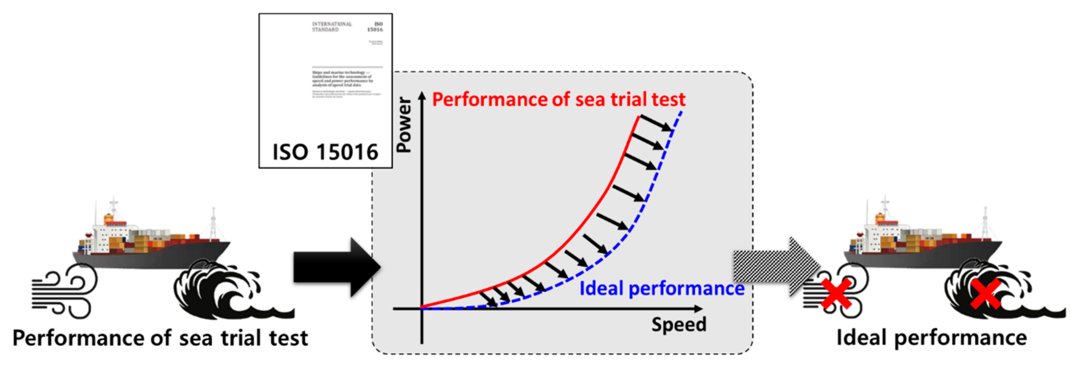
3.1. ISO 15016:2002 for the Assessment of Speed and Power Performance
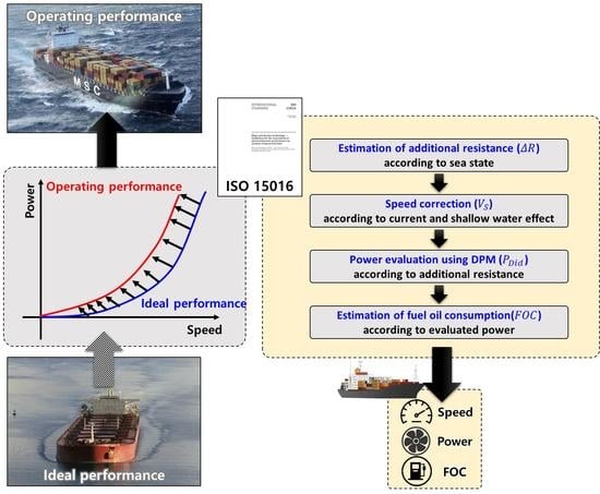
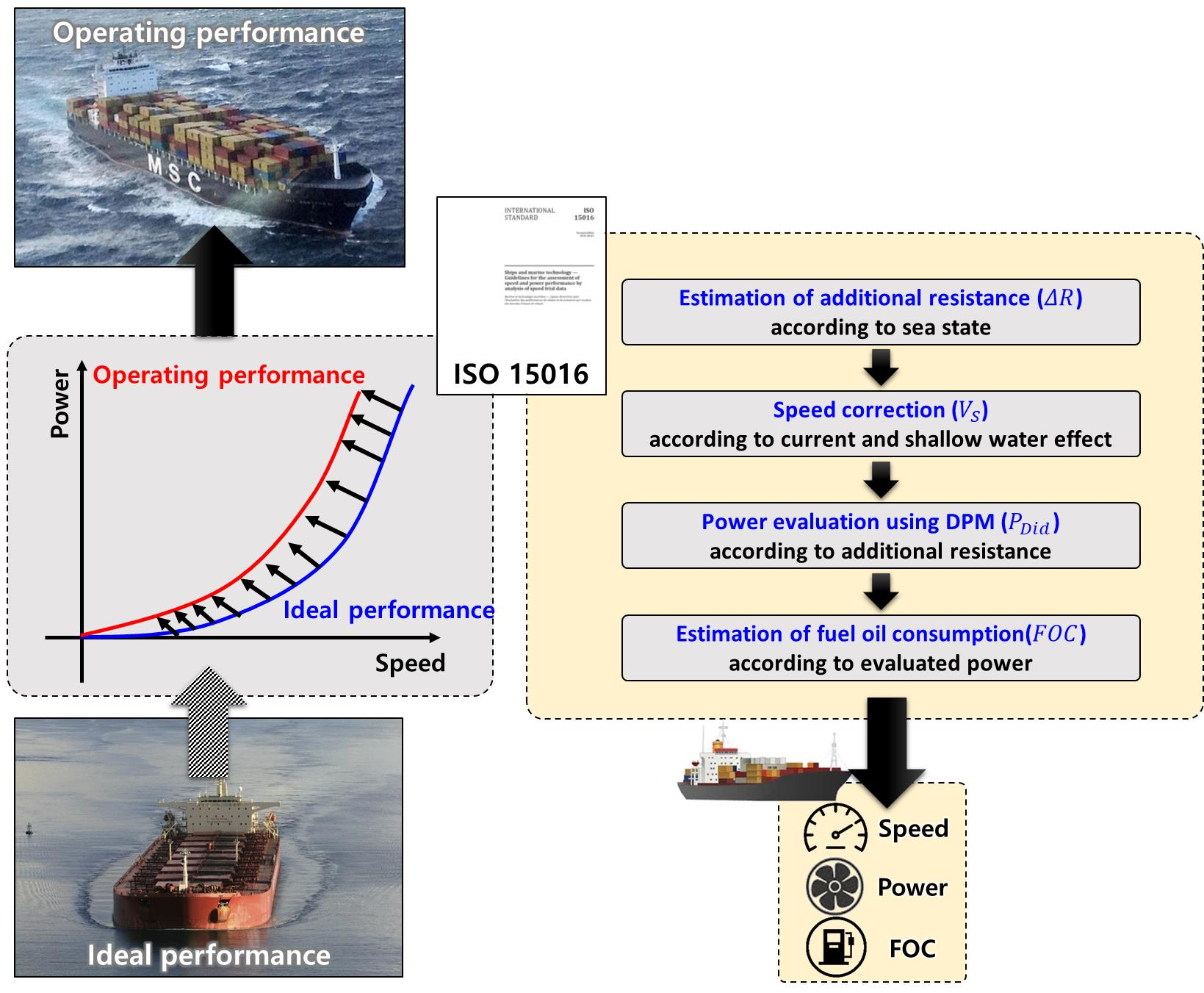
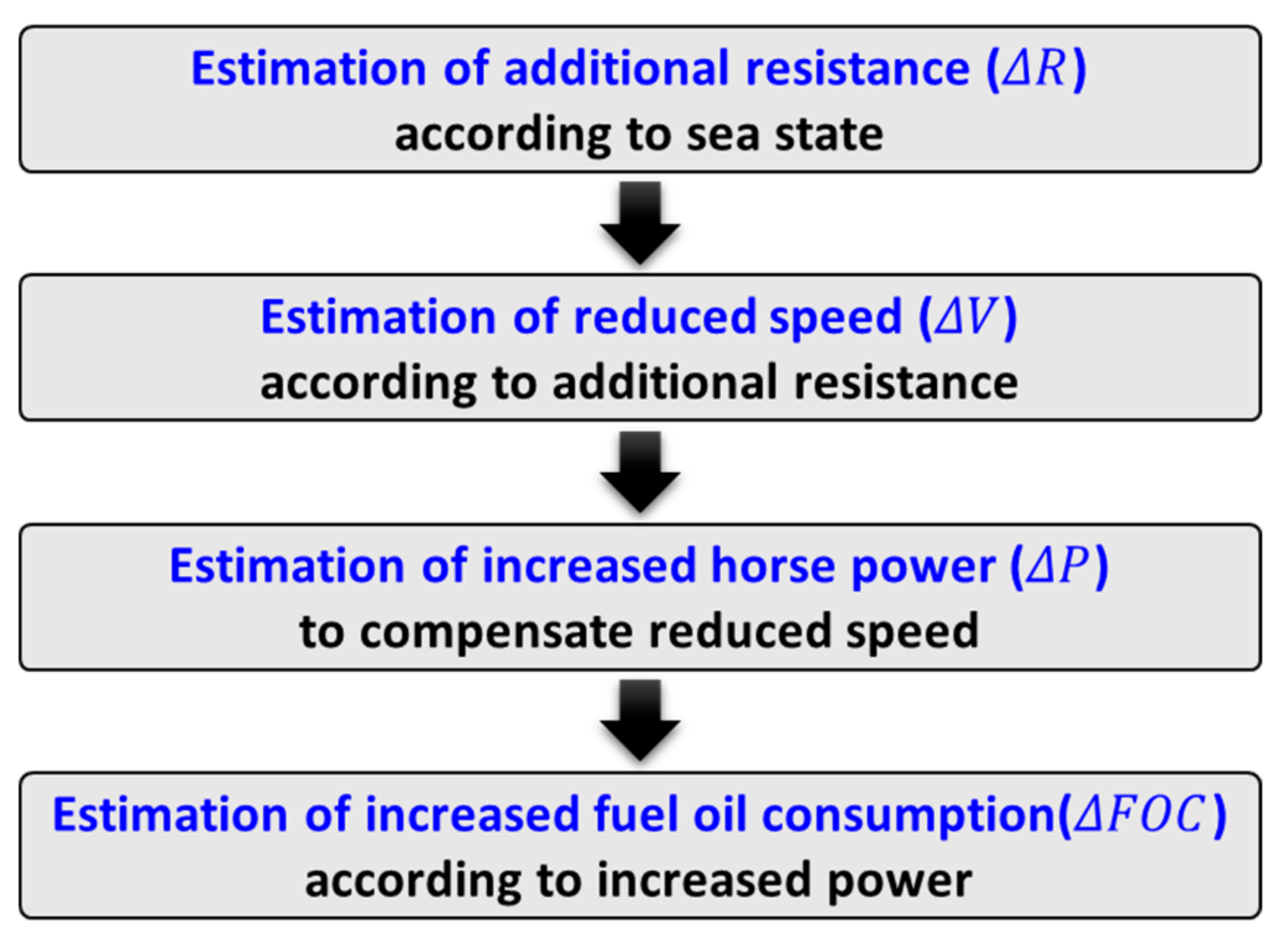
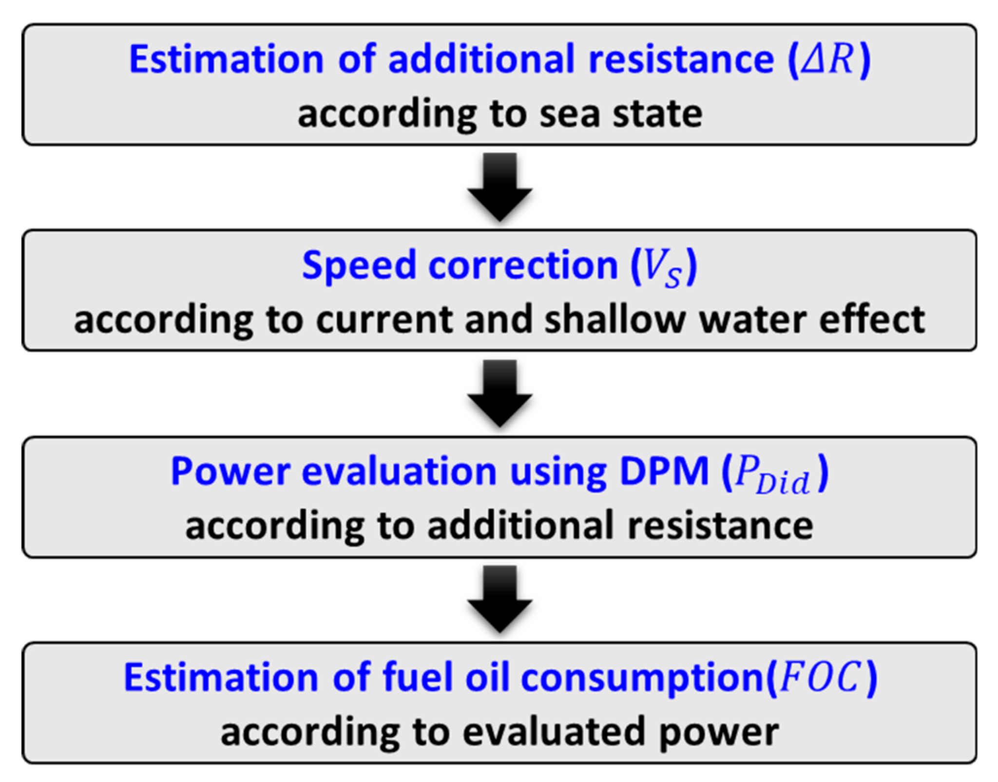
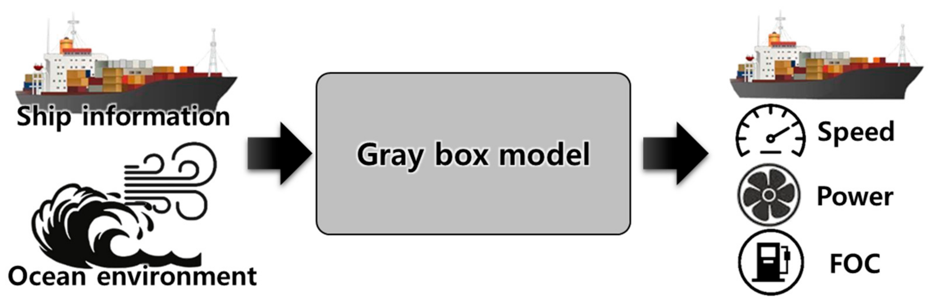
3.2. Method for the Estimation of Fuel Oil Consumption Using ISO 15016:2015
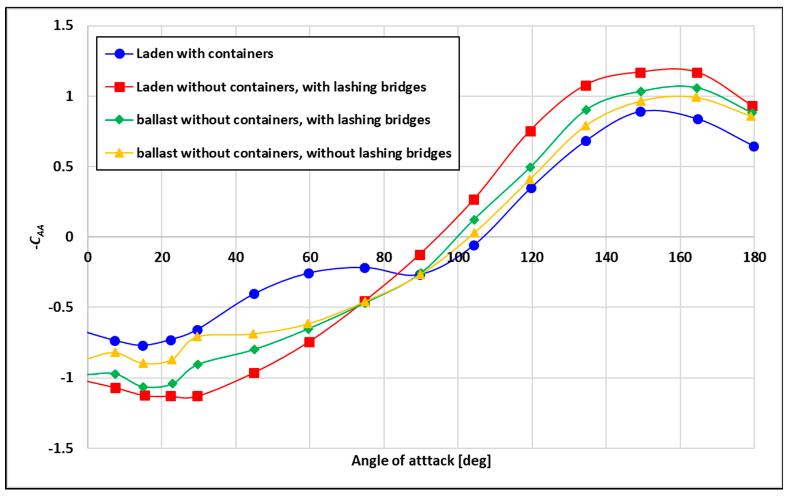
3.2.1. Estimation of Additional Resistance
3.2.2. Speed Correction for Current and Shallow Water Effects
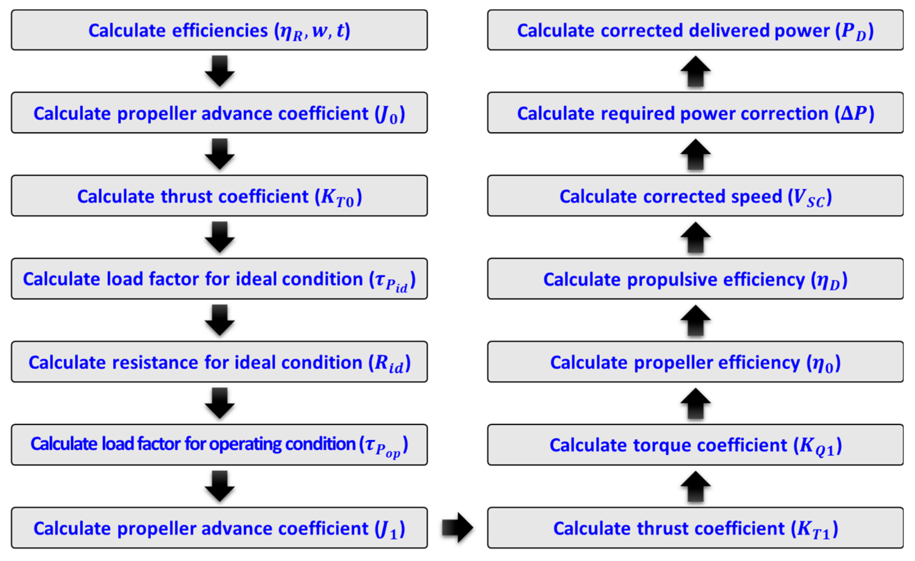
3.2.3. Power Evaluation Using the DPM
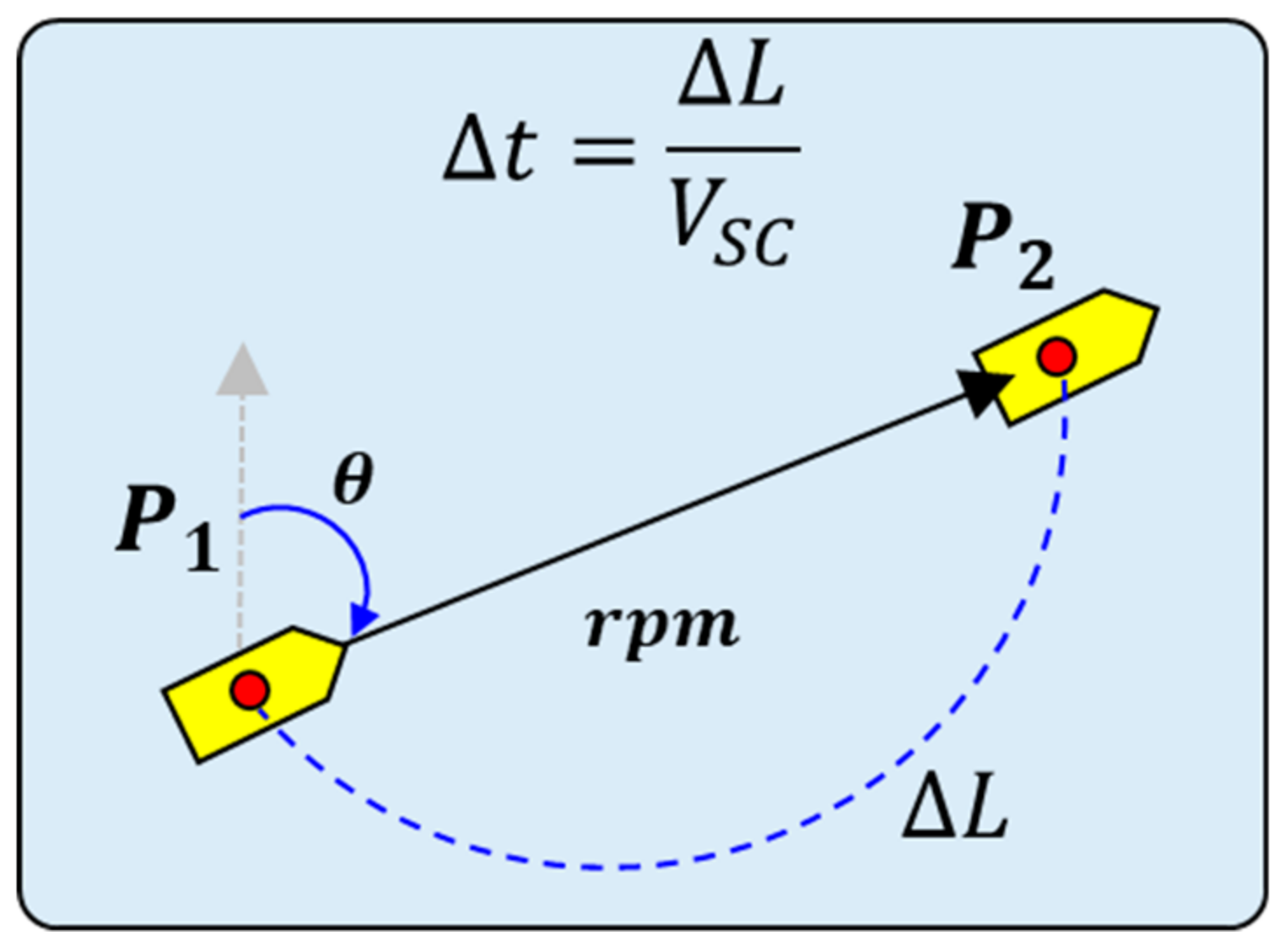
3.2.4. Estimation of Fuel Oil Consumption
4. Application
4.1. Case Definition
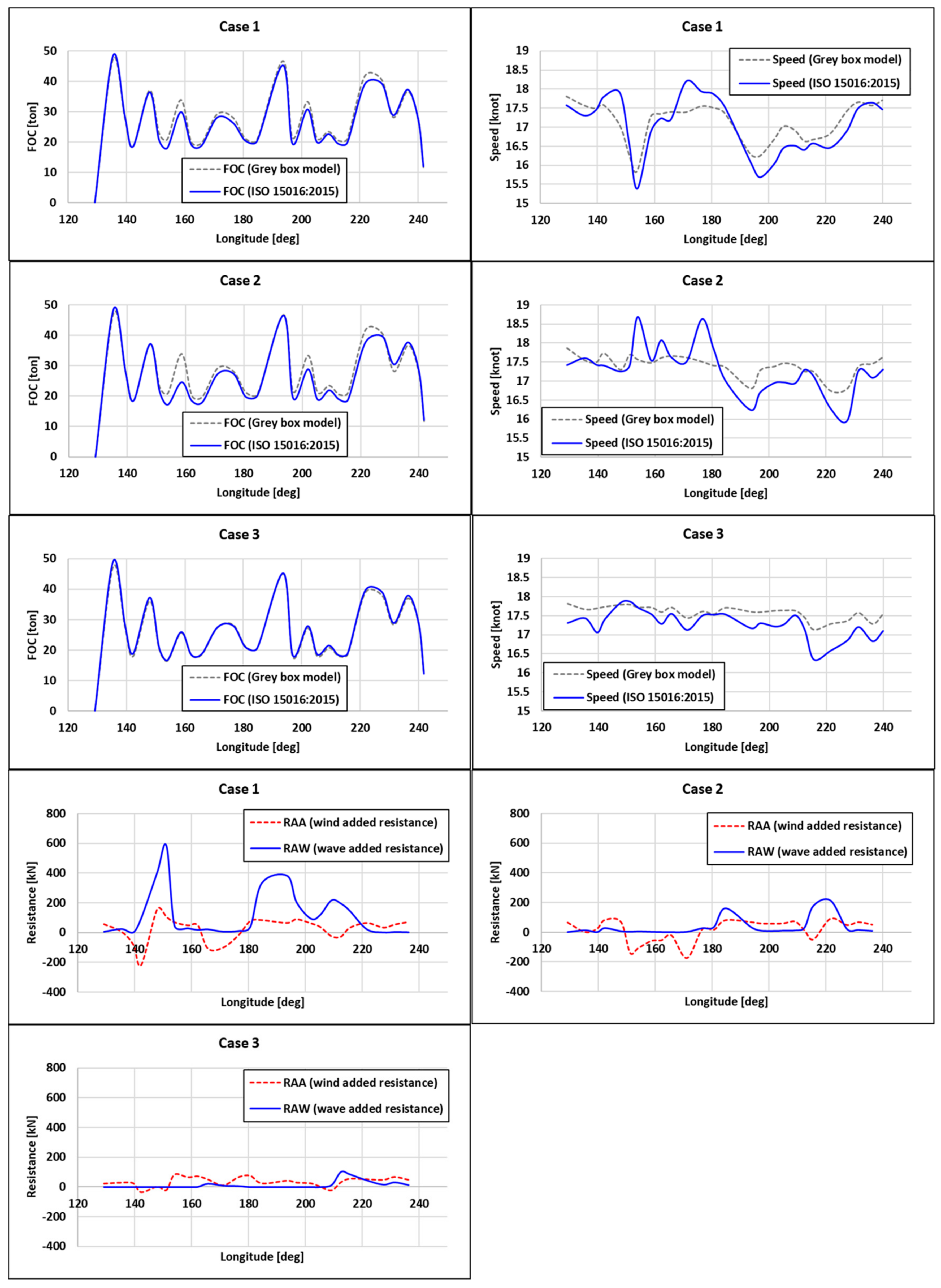
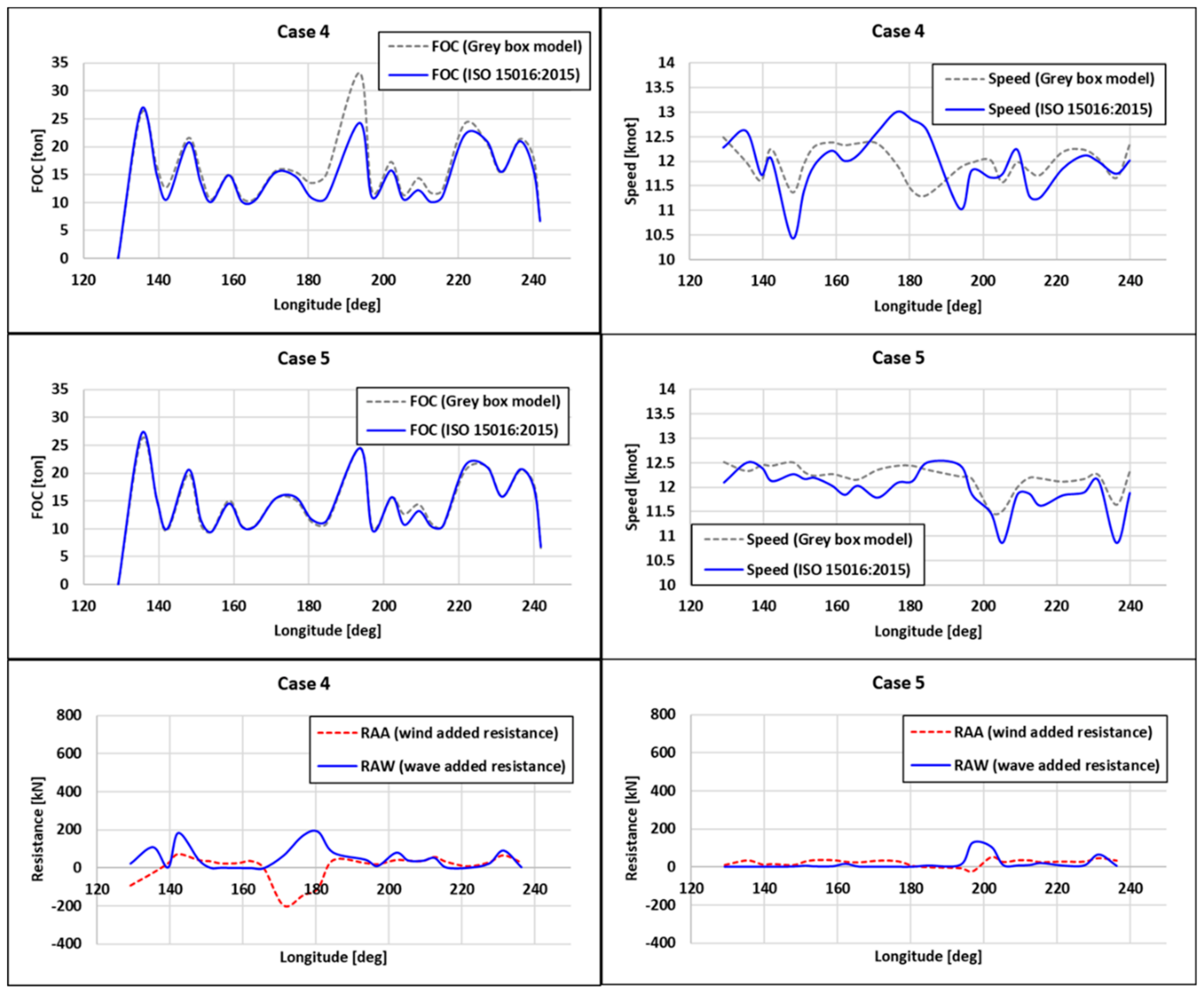
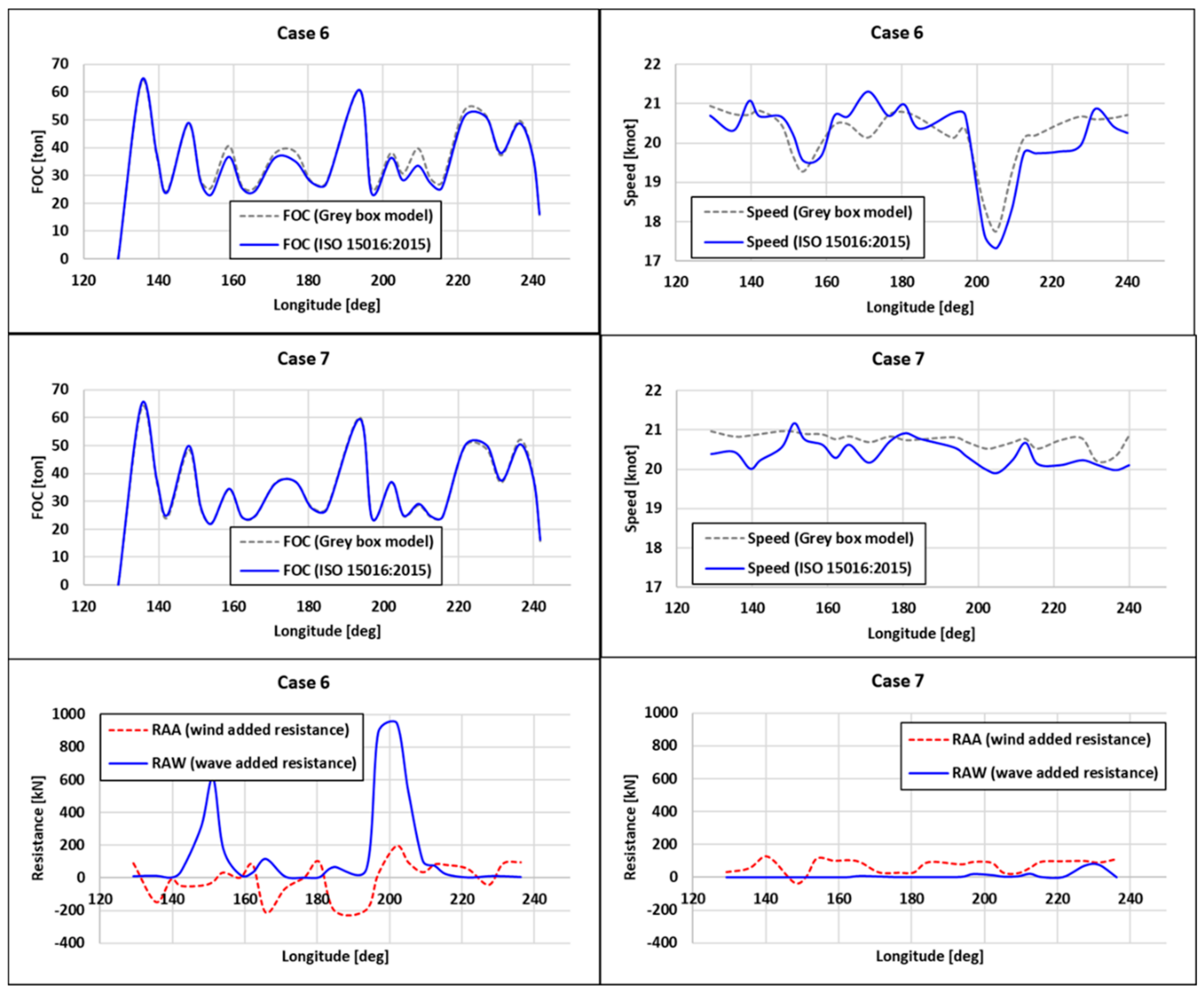
4.2. Case Studies
5. Conclusions and Future Work
Author Contributions
Funding
Conflicts of Interest
References
- Avgouleas, K.; Sclavounos, P.D. Fuel-Efficient Ship Routing. Nat. Sci. Math. 2014, 5, 39–72. [Google Scholar]
- Weber, T. The Importance of Weather Routing in Fuel-Efficient Shipping; Vessel Performance Optimization (VPO): London, UK, 2018. [Google Scholar]
- ISO. ISO 15016:2015-Ship and Marine Technology-Guidelines for the Assessment of Speed and Power Performance by Analysis of Speed Trial Data; ISO: Geneva, Switzerland, 2015. [Google Scholar]
- Joo, S.-Y.; Cho, T.-J.; Cha, J.-M.; Yang, J.-H.; Kwon, Y.-K. An Economic Ship Routing System Based on a Minimal Dynamic-cost Path Search Algorithm. KIPS Trans. Comput. Commun. Syst. 2012, 1, 79–86. [Google Scholar] [CrossRef][Green Version]
- Bang, S.-H.; Kwon, Y.-K. Economic Ship Routing System by a Path Search Algorithm Based on an Evolutionary Strategy. J. Korean Inst. Commun. Inf. Sci. 2014, 39, 767–773. [Google Scholar] [CrossRef][Green Version]
- Townsin, R.L.; Kwon, Y.J. Estimating the Influence of Weather on Ship Performance; Wind Press: Milano, Italy, 1993; Volume 135, pp. 191–209. [Google Scholar]
- Lin, Y.-H.; Fang, M.-C.; Yeung, R.W. The optimization of ship weather-routing algorithm based on the composite influence of multi-dynamic elements. Appl. Ocean Res. 2013, 43, 184–194. [Google Scholar] [CrossRef]
- Vettor, R.; Soares, C.G. Development of a ship weather routing system. Ocean Eng. 2016, 123, 1–14. [Google Scholar] [CrossRef]
- Park, J.; Kim, N. Two-Phase Approach to Optimal Weather Routing Using Real-Time Adaptive A* Algorithm and Geometric Programming. J. Ocean Eng. Technol. 2015, 29, 263–269. [Google Scholar] [CrossRef]
- Roh, M.-I. Determination of an economical shipping route considering the effects of sea state for lower fuel consumption. Int. J. Nav. Arch. Ocean Eng. 2013, 5, 246–262. [Google Scholar] [CrossRef]
- Wei, S.; Zhou, P. Development of a 3D Dynamic Programming Method for Weather Routing. In Methods and Algorithms in Navigation: Marine Navigation and Safety of Sea Transportation; CRC Press: Boca Raton, FL, USA, 2011; Volume 6, pp. 181–187. [Google Scholar] [CrossRef]
- Chen, H. Voyage Optimization Supersedes Weather Routing; Jeppesen Marine Inc.: Denver, CO, USA, 2011; pp. 1–11. [Google Scholar]
- ISO. ISO 15016:2002-Ship and Marine Technology—Guidelines for the Assessment of Speed and Power Performance by Analysis of Speed Trial Data; ISO: Geneva, Switzerland, 2002. [Google Scholar]
- Eniram. Fuel Saving; Eniram: Helsinki, Finland, 2008. [Google Scholar]
- Samsung. Samsung Heavy Industries Energy Efficiency Management System; Samsung: Seoul, Korea, 2017. [Google Scholar]
- Schlinkert, G. StormGeo Route Planning for Different Ship Types and Speeds; StormGeo: Bergen, Norway, 2019. [Google Scholar]
- SeaRates. DP World SeaRates Route Planner; SeaRates: Dubai, UAE, 2020. [Google Scholar]
- Nakamura, S.; Naito, S. Nominal speed loss and propulsive performance of a ship in waves. J. Soc. Nav. Archit. Kansai 1972, 166, 25–34. [Google Scholar]
- ITTC. ITTC Recommended Procedures and Guidelines, Analysis of Speed/Power Trial Data. 7.5-04-01-01.2; ITTC: Nantes, France, 2014. [Google Scholar]
- Sea Trial Analysis JIP. Recommended Analysis of Speed Trials; MARIN: Wageningen, The Netherlands, 2006. [Google Scholar]
- Van den Boom, H.; Huisman, H.; Mennen, F. New Guidelines for Speed/Power Trials: Level Playing Field Established for IMO EEDI; SWZ/Maritime: Rotterdam, The Netherlands, 2013; pp. 1–11. [Google Scholar]
- Stewart, R.H. Chapter 16—Ocean Waves. In Introduction to Physical Oceanography; Texas A&M University: College Station, TX, USA, 2008. [Google Scholar]
- Holtrop, J.; Mennen, G. An approximate power prediction method. Int. Shipbuild. Prog. 1982, 29, 166–170. [Google Scholar] [CrossRef]
- Bernitsas, M.M.; Ray, D.; Kinley, P. Kt, Kq and Efficiency Curves for the Wageningen B-Series Propellers; The University of Michigan: Ann Arbor, MI, USA, 1981. [Google Scholar]
- Kroll, A. Grey-box models: Concept and application. In New Frontiers in Computational Intelligence and Its Application; IOS Press: Amsterdam, The Netherlands, 2000; Volume 57, pp. 42–51. [Google Scholar]


| Research | Method for Estimating Fuel Oil Consumption | Application |
|---|---|---|
| Joo et al. [4] | Townsin-Kwon method | All ships |
| Bang and Kwon [5] | Townsin-Kwon method | All ships |
| Lin et al. [7] | Polynomial function | All ships |
| Vettor and Soares [8] | Polynomial function | All ships |
| Park et al. [9] | 2nd order polynomial function | All ships |
| Roh [10] | ISO 15016:2002 | All ships |
| Wei and Zhou [11] | ISO 15016:2002 | All ships |
| Chen [12] | ISO 15016:2002 | All ships |
| Eniram [14] | Statistical method | Specific ships |
| SHI [15] | Statistical method | Specific ships |
| This study | ISO 15016:2015 | All ships |
| Particulars | Value |
|---|---|
| Length between perpendiculars | 237 m |
| Breadth | 37.5 m |
| Depth | 22 m |
| Draft | 11 m |
| Deadweight | 59,000 ton |
| RPM at NCR | 77 rpm |
| Cases | Departure | Arrival | Departure Date | Engine RPM | Weather Condition |
|---|---|---|---|---|---|
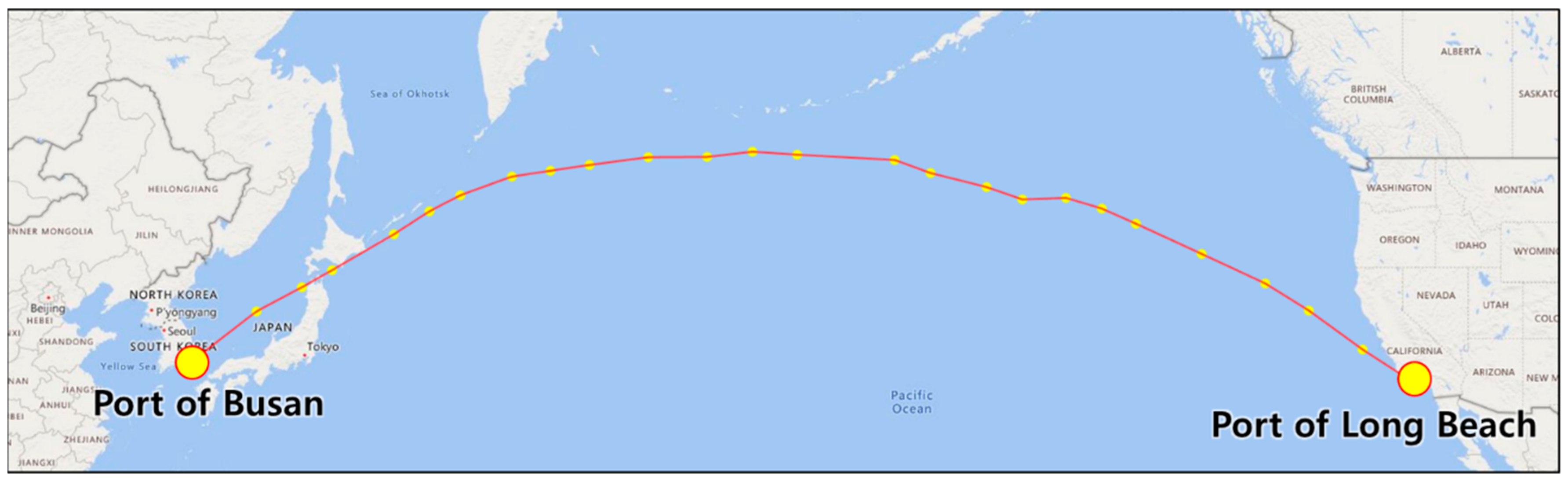
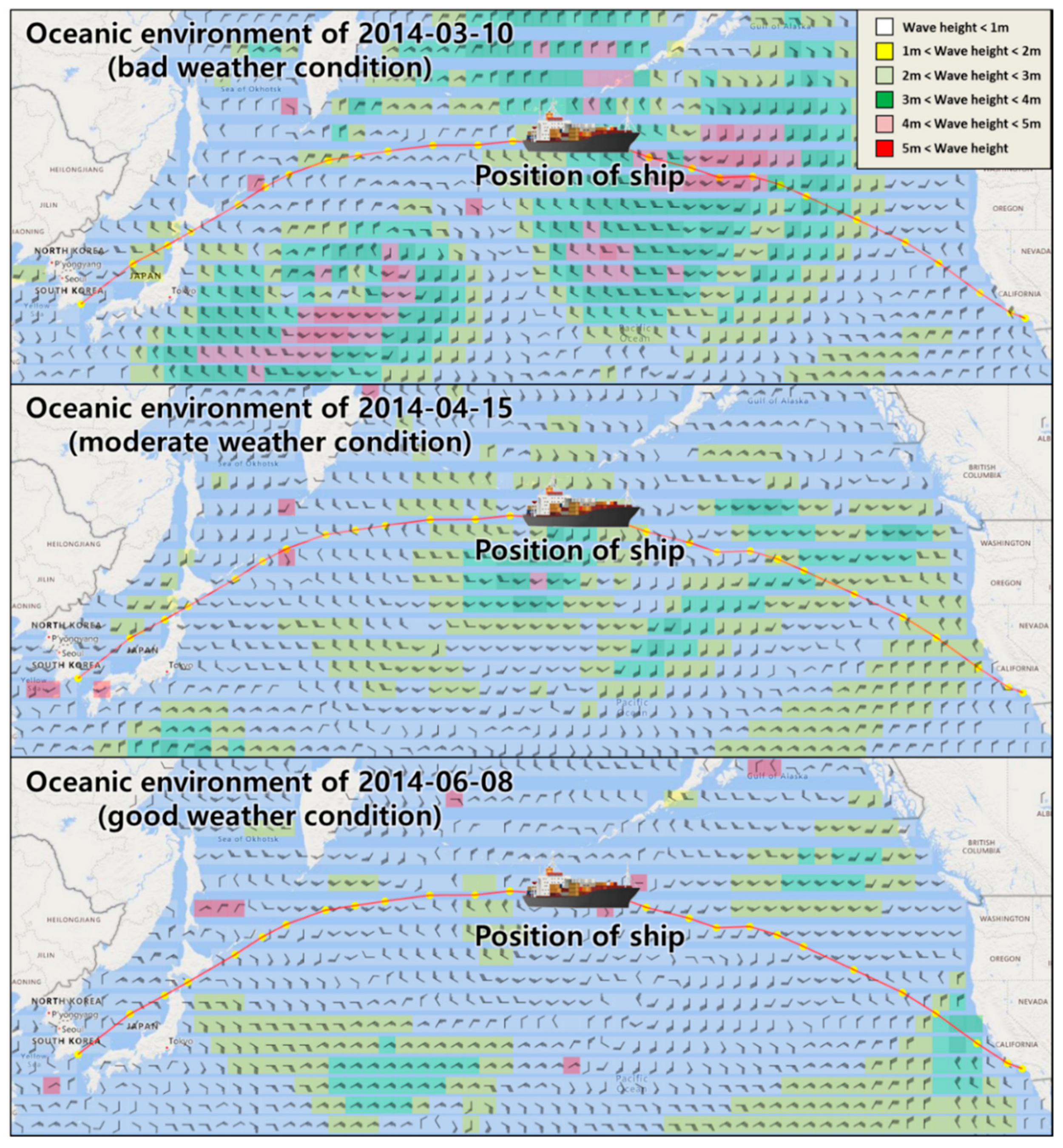
| Case 1 | Port of Busan, South Korea | Port of Long Beach, USA | 3 March 2014, 18:00 | 77 (normal steaming) | Bad |
| Case 2 | 8 April 2014, 18:00 | Moderate | |||
| Case 3 | 1 June 2014, 18:00 | Good | |||
| Case 4 | 3 March 2014, 18:00 | 55 (slow steaming) | Bad | ||
| Case 5 | 1 June 2014, 18:00 | Good | |||
| Case 6 | 3 March 2014, 18:00 | 90 (fast steaming) | Bad | ||
| Case 7 | 1 June 2014, 18:00 | Good |
| Cases | Methods | TFOC (ton) | Average Speed (knot) | Arrival Time | Engine RPM |
|---|---|---|---|---|---|
| Case 1 | Gray box model | 721.4 (100%) | 17.47 (100%) | 16 March 2014, 06:25 | 77 (normal steaming) |
| ISO 15016:2015 | 694.3 (96.2%) | 17.35 (99.3%) | 16 March 2014, 08:24 | ||
| Case 2 | Gray box model | 692.4 (100%) | 17.73 (100%) | 21 April 2014, 01:56 | |
| ISO 15016:2015 | 685.9 (99.1%) | 17.56 (99.0%) | 21 April 2014, 04:47 | ||
| Case 3 | Gray box model | 674.0 (100%) | 17.91 (100%) | 13 June 2014, 22:56 | |
| ISO 15016:2015 | 685.9 (101.8%) | 17.56 (98.0%) | 14 June 2014, 04:46 | ||
| Case 4 | Gray box model | 418.3 (100%) | 12.20 (100%) | 21 March 2014, 16:03 | 55 (slow steaming) |
| ISO 15016:2015 | 381.7 (91.3%) | 12.20 (100.0%) | 21 March 2014, 16:11 | ||
| Case 5 | Gray box model | 381.7 (100%) | 12.44 (100%) | 19 June 2014, 07:48 | |
| ISO 15016:2015 | 382.2 (100.1%) | 12.18 (97.9%) | 19 June 2014, 16:43 | ||
| Case 6 | Gray box model | 949.4 (100%) | 20.64 (100%) | 14 March 2014, 08:12 | 90 (fast steaming) |
| ISO 15016:2015 | 916.6 (96.5%) | 20.53 (99.4%) | 14 March 2014, 09:38 | ||
| Case 7 | Gray box model | 898.5 (100%) | 21.12 (100%) | 12 June 2014, 02:29 | |
| ISO 15016:2015 | 906.6 (100.9%) | 20.75 (98.2%) | 12 June 2014, 06:50 | ||
| Average ratio | 97.9% | 98.9% | |||
© 2020 by the authors. Licensee MDPI, Basel, Switzerland. This article is an open access article distributed under the terms and conditions of the Creative Commons Attribution (CC BY) license (http://creativecommons.org/licenses/by/4.0/).
Share and Cite
Kim, K.-S.; Roh, M.-I. ISO 15016:2015-Based Method for Estimating the Fuel Oil Consumption of a Ship. J. Mar. Sci. Eng. 2020, 8, 791. https://doi.org/10.3390/jmse8100791
Kim K-S, Roh M-I. ISO 15016:2015-Based Method for Estimating the Fuel Oil Consumption of a Ship. Journal of Marine Science and Engineering. 2020; 8(10):791. https://doi.org/10.3390/jmse8100791
Chicago/Turabian StyleKim, Ki-Su, and Myung-Il Roh. 2020. "ISO 15016:2015-Based Method for Estimating the Fuel Oil Consumption of a Ship" Journal of Marine Science and Engineering 8, no. 10: 791. https://doi.org/10.3390/jmse8100791
APA StyleKim, K.-S., & Roh, M.-I. (2020). ISO 15016:2015-Based Method for Estimating the Fuel Oil Consumption of a Ship. Journal of Marine Science and Engineering, 8(10), 791. https://doi.org/10.3390/jmse8100791