Article

Analysis and Selection of Deployment Methods for a Wave Glider System

College of Engineering, Ocean University of China, Qingdao 266100, China
*
Author to whom correspondence should be addressed.
J. Mar. Sci. Eng. 2020, 8(7), 529; https://doi.org/10.3390/jmse8070529
Submission received: 9 June 2020 / Revised: 7 July 2020 / Accepted: 13 July 2020 / Published: 17 July 2020
(This article belongs to the Special Issue Advances in Wave Energy Harvesting)

Abstract

:
A wave glider is a novel unmanned marine vehicle which can convert marine energy into kinetic energy. In practice, it is crucial for the wave glider system to deploy into the ocean environment efficiently and safely. Hence, the present work establishes the wave glider motion equations to analyze the deployment method. Firstly, the wave glider model is simplified in the vertical plane and the cable model is defined as mass nodes connected with a massless spring. Then, two typical deployment methods (Method 1 and Method 2) are proposed based on the multibody dynamic method, and the numerical simulation model is established to investigate the kinematic performance of two deployment methods. Lastly, the dynamic characteristic analysis is conducted to select the determined deployment method. We explain the practical advantages of Method 1, which would provide the reference for the deployment method selection.

1. Introduction

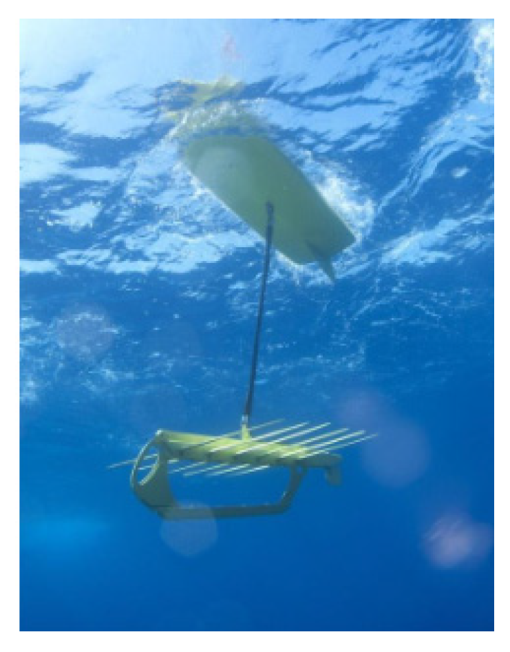
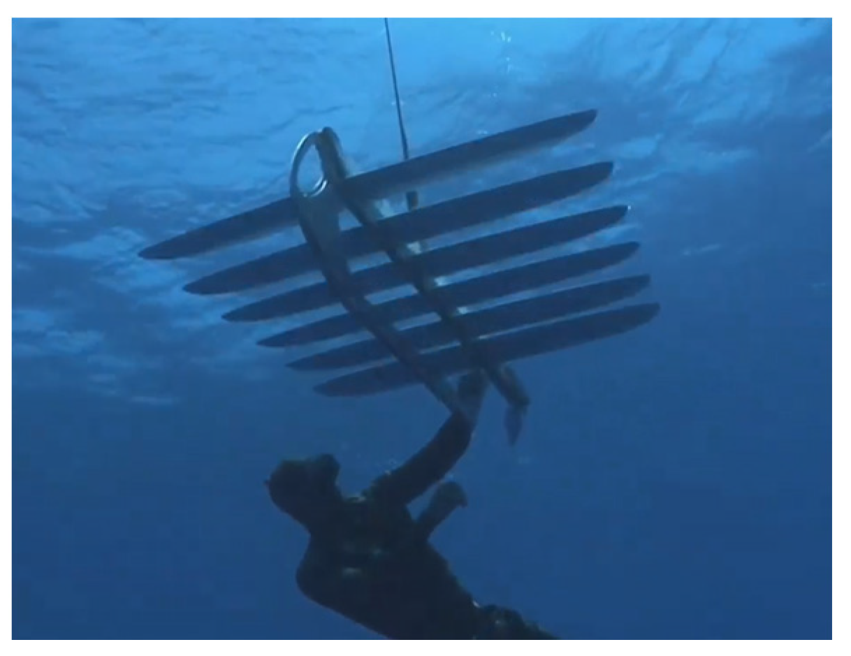
A wave glider is widely applied in the field of ocean environmental monitoring as an innovative unmanned marine vehicle. The unique two-body structure is composed of a submerged propulsor (glider) and a surface floater (float), which are connected by a flexible cable (Figure 1 and Figure 2). A wave glider manifests great advantages in propulsive performance after comparing with other traditional sea-going vehicles; for example, it cruises automatically, conducts low-cost surveying and is environmentally friendly [1,2,3].
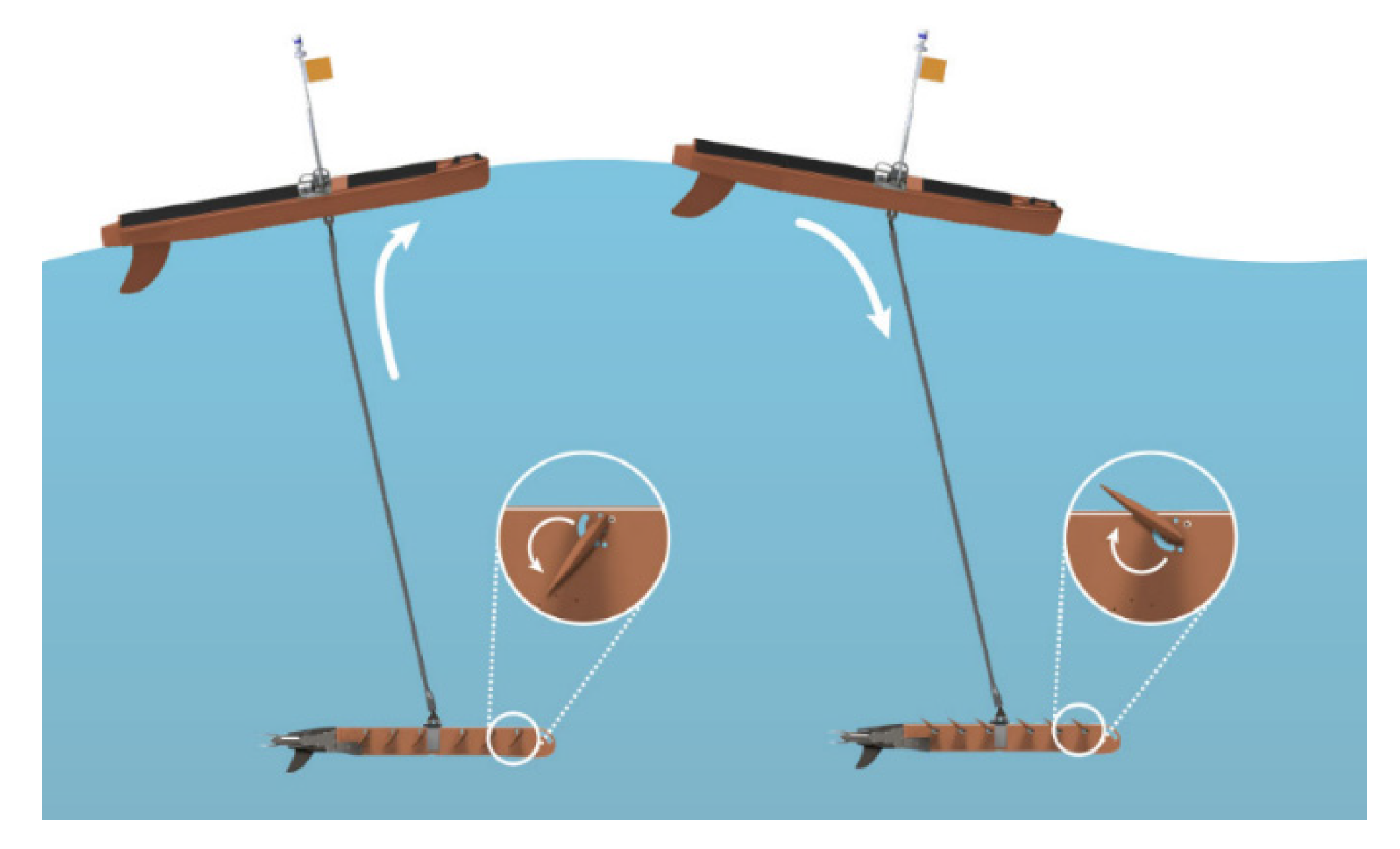
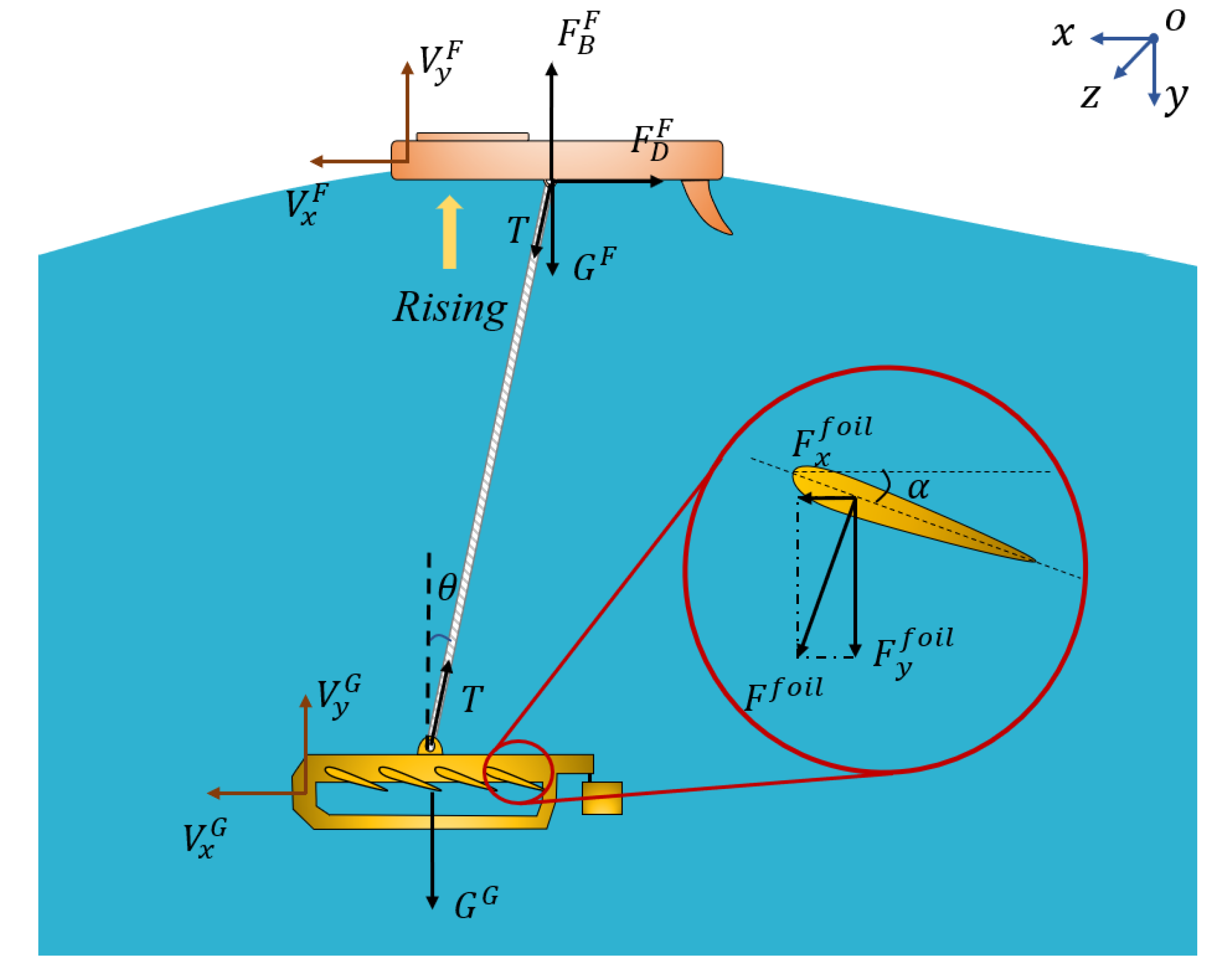
The wave glider float is always affected by surface waves and is a submerged glider. During the heave motion process, the wave glider rises and sinks with waves. At the same time, the cable is used to deliver force between the float and glider. The hydrodynamic force is generated by relative motion between hydrofoils and seawater, and a forward thrust is generated in the process. The principle of the wave glider operating is shown in Figure 3.
Nowadays, the study of the dynamics performance of wave gliders has attracted scholars’ attention for many years, and a great number of efforts have been made to analyze and optimize the dynamics performance of wave gliders.
Kraus [4] applied the Newton Euler method to establish a 6-DOF (degrees of freedom) realizable model of wave glider, which expanded the mathematical model from a traditional 2D model to 3D. Caiti et al. [5] presented a Lagrangian approach in designing a novel class of hybrid underwater wave gliders; this proposed vehicle was able to accomplish both surface and submarine assignments. Qi et al. [6] and Zhou et al. [7] simplified a multi-body dynamics model of UWGs (unmanned wave gliders) to a 2-DOF system based on Kane’s equations. These specific modeling methods are widely used by many researchers and provided much assistance for analyzing motion features of wave gliders.
Feng et al. [8] established a cable model of a wave glider by considering the connection characteristics such as a rigid rod, cable, multi-link chain and elastic rod. The results showed that the propulsion performance with different connection types of the wave glider is slightly different. Zhang and Xu [9] studied the motion relationship between the float and the submarine glider by MATLAB (Matrix Laboratory, a business software developed by The MathWorks, Inc. Natick, USA), and the cable connecting was divided into several segments. It is very helpful to model the cable. Wang [10] proposed a UWGs dynamic model after considering the influences of the flexible umbilical. It was found that this established model is reasonable when considering the longitudinal and rotary motions.
In order to predict the wave glider dynamics performance in head seas, Yang et al. [11] studied the tandem hydrofoils as a system by computational fluid dynamics (CFD) after considering passive eccentric rotation of hydrofoil. The results indicate that the surge force acting on the float and the passive eccentric rotation law of the hydrofoils have the major impact on the propulsion performance. The motion control approach of a wave glider mainly uses proportional-integral-derivative (PID) Control [12,13]. These research works provide the ideas of dynamic modeling of wave glider by identification algorithms.
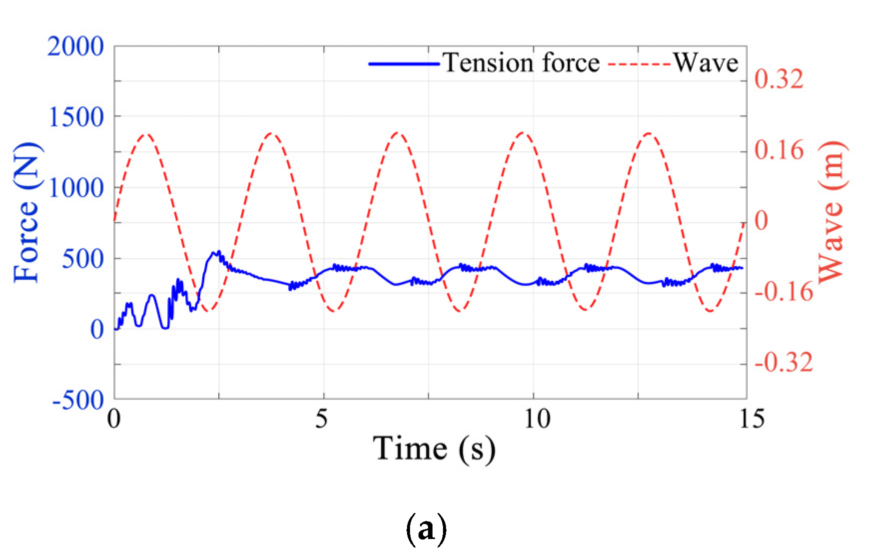
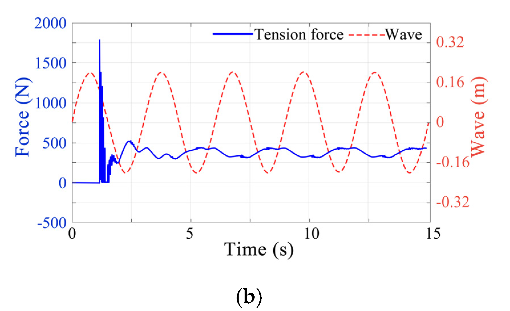
The results obtained above are of great significance for motion analysis and performance optimization of a wave glider. However, previous research did not investigate the deployment process, which may have potential security issues. Thrust is generated by the submerged glider when the wave glider is released and the force caused by the surrounding medium acts on the float. The flexible cable state changes from slack to tense during the deployment process. It should be emphasized that the forces acting on the float and submerged glider are extremely great when the cable reaches the maximum length, and the wave glider system will probably be damaged at that moment. In addition, instruments installed on the wave glider may fall off due to excessive impact. Therefore, it is necessary to select the optimal deployment method for avoiding the negative impact on a wave glider.
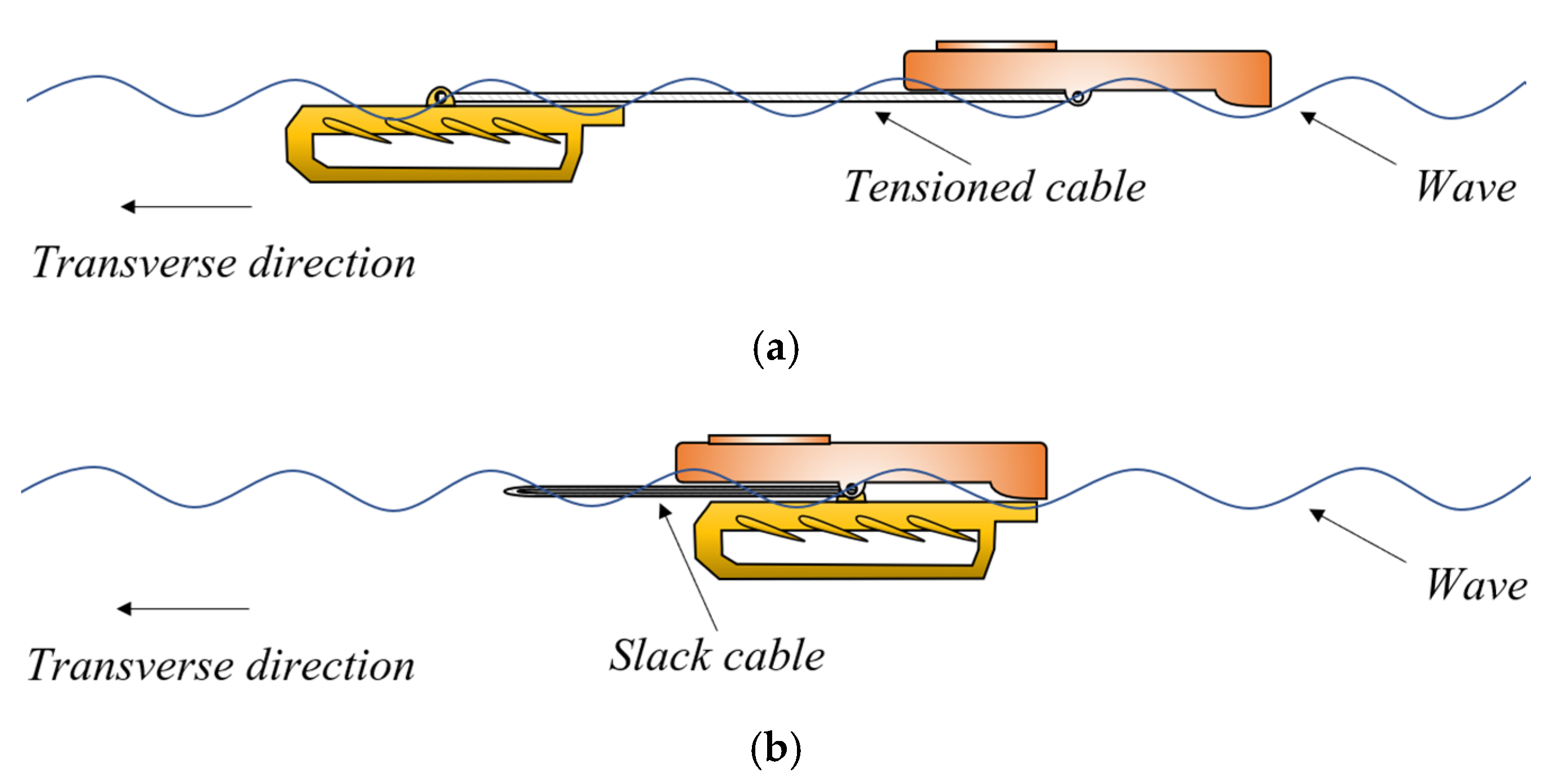
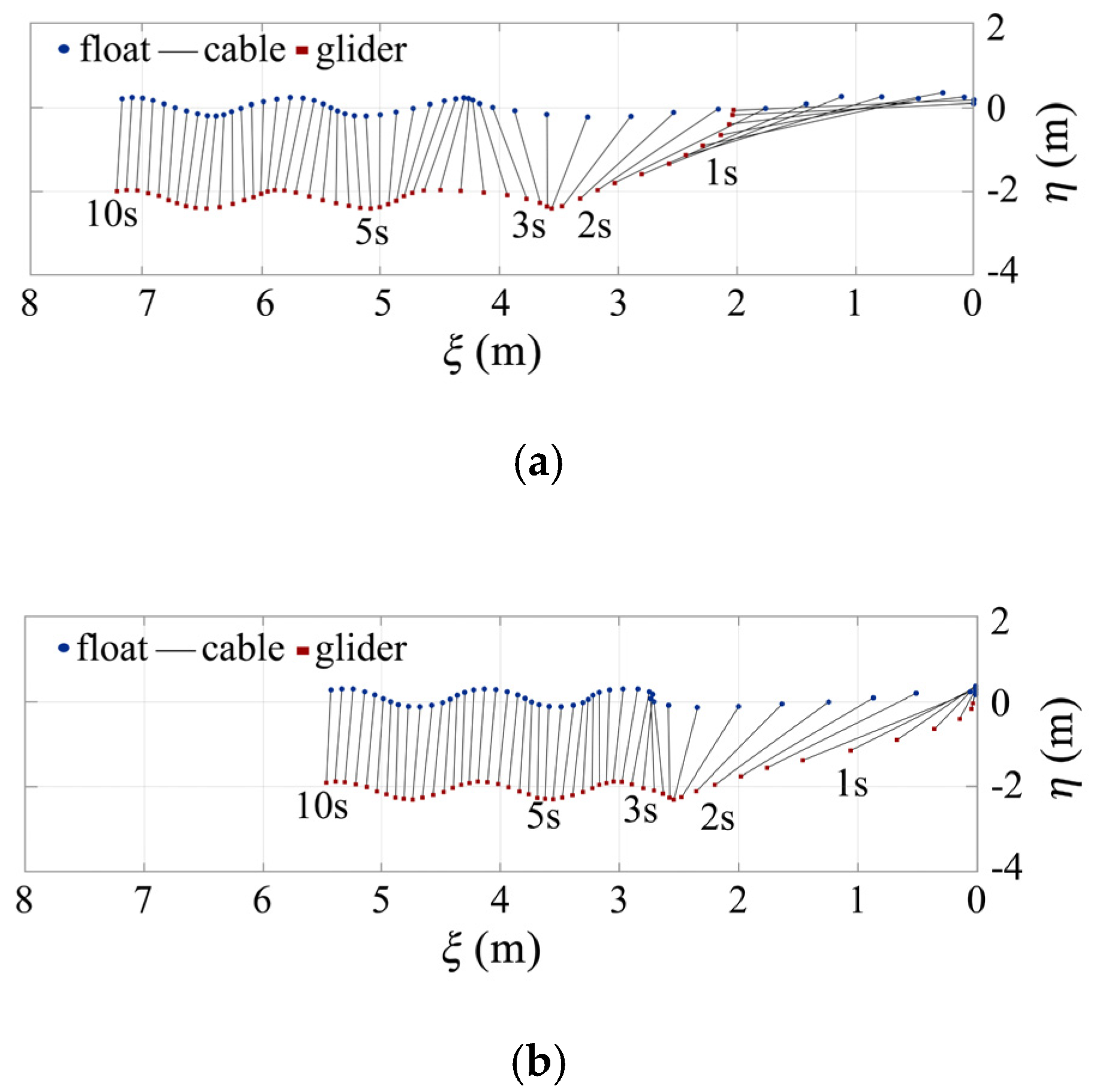
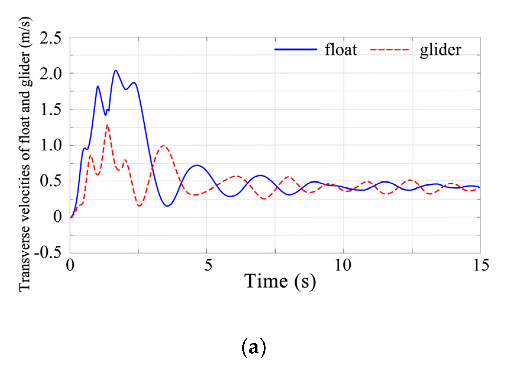
In a real-world application, two typical methods (Method 1 and Method 2) are widely used to deploy wave gliders into ocean environments. The specific deployment process of Method 1 is shown in 
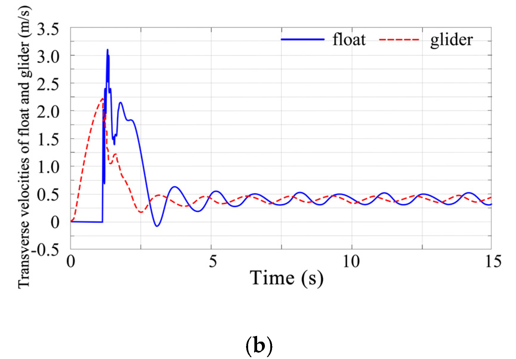
Figure 4a. Firstly, the wave glider is separated from two components (the float and the glider), which are connected by a tensioned cable. Then, these components will sink on account of the gravity effect. Hydrofoils rotate in degrees due to the hydrodynamic impact after contact with seawater. The wave glider system is subsequently propelled going forward by the hydrodynamic. Similarly, the float and glider are released at the same time, and the cable remains slack until the cable length is up to the maximum in Figure 4b. However, the deployment method of Method 2 is arranged up and down.
In this paper, the wave glider model is simplified in the vertical plane and the cable model is assumed as mass nodes connected with a massless spring. The motion equations of wave gliders are firstly established by a multibody dynamics method to comprehensively analyze the dynamic performance of two typical deployment methods, and the results will be obtained and compared by the numerical simulation method.

2. Multibody Dynamic Models of Wave Gliders

The motion of a wave glider is susceptible to the variety of surroundings because it always couples with different sea conditions. Therefore, it is extremely hard to establish a completely accurate model. In order to study the deployment methods discussed above, a simplified model is constructed to reflect the deployment situations reasonably, and the restrictions and hypothesis are proposed as follows:
  • Heave and sway motion are only considered for the float and glider, and the model is established in a vertical plane.
  • The mass center of the float and glider is located on the hinged joint. The cable has no effects on the wave glider system when it is slack.
  • The hydrodynamics parameters are calculated based on potential theory, thus, this model is not adapted to extreme sea states.
  • Concentrated forces are calculated to act on the wave glider system directly and the relative motion between seawater and the wave glider is neglected.
  • The vortexes and wakes caused by the hydrofoil’s rotation are neglected.
Cong et al. [14] performed the mathematical model to express an approximate heave motion of the wave by the wave energy spectrum theory and it is formulated as follows:
y ( x , t ) = A sin ( k x ω t + φ )
where A is half of the wave height, k is sequence number of the wave, ω is wave circular frequency, and φ is initial phase.
The corresponding coordinate systems of the wave glider are presented in Figure 5, which is the so-called earth-fixed frame as o x y . Force analysis of the wave glider is also shown in this figure. The surface float is regarded as an object with concentrated mass which is affected by the wave force without considering other external factors. The hydrofoils fixed on the glider provides active force for the system, and the rudder adjustment plays an important role in keeping the float and glider in a vertical plane. As shown in Figure 5, this figure presents the force condition, which acts on the wave glider with a wave rising process. The cable state transforms from slack to tense during the deployment process.
The velocities of the float v F and the glider v G are obtained as:
{ v F = v x F i + v y F ( j ) v G = v x G i + v y G ( j )
where i and j are the unites vector along the positive direction of the x-axis and y-axis, respectively. The absolute speed of the float, cable and glider is v # * , the right-superscript * is the object aimed to express, and the right-subscript # denotes a certain coordinate axis.
The location of the float and glider in an earth-fixed frame are formulated as follows:
ξ ˙ F = v x F         η ˙ F = v y F
ξ ˙ G = v x G         η ˙ G = v y G
where ξ F and   η F are, respectively, transverse and longitudinal coordinates of the float in the earth-fixed frame; ξ G and   η G are, respectively, transverse and longitudinal coordinates of the glider in the earth-fixed frame.
Therefore, the distance from float to glider is derived as:
l = ( ξ F ξ G ) 2 + ( η F η G ) 2
The active force acting on the float consists of gravity ( G F ), buoyancy ( F B F ), wave resistance ( F D F ) and tension force ( T ), which are expressed as follows:
{ F x F = ( T sin θ F D F ) i F y F = ( G F F B F + T cos θ ) j
The glider would keep sinking in still water because its density is almost 7.85 times than that of water, so the real buoyancy would not change the dynamic performance. Since it would make a negligible impact on the whole system, the wave glider buoyancy can be ignored. The active force on the glider includes the gravity ( G G ), hydrodynamic force on a single hydrofoil ( F f o i l ), and tension force ( T ), which can be written as follows:
{ F x G = ( n F f o i l sin α + T sin θ ) i F y G = ( G G + n F f o i l cos α T cos θ ) j
When a wave glider goes forward, the float is subject to water resistance in the horizontal direction. The transverse force hindering movement is simplified as follows:
F D F = 1 2 C D ρ S 1 F ( v x F ) 2 ( i )
where C D are drag coefficients, ρ is the density of seawater, S 1 F is the projected area of the immersed part in the transverse direction.
The float buoyancy is affected by mass and immersed volume. In addition, the wave motion equation is supplemented with the buoyancy equation to consider a continuously changed wave state. It can be expressed as follows:
F B F = ρ S 2 F ( y i n i t i a l y 1 + y ( x , t ) ) g ( j )
where S 2 F is the cross-sectional area of the float, y i n i t i a l is the initial draft, and y 1 is the variation of draft.
The hydrofoils fixed on the glider generate propulsive force for the system; the mode of F f o i l is as follows:
{ F f o i l = 1 2 C D ρ S f o i l ( v y G cos α v x G sin α ) 2 F f o i l = F x f o i l i + F y f o i l j
where S f o i l is total area of hydrofoils, α is the angle of attack, F x f o i l and F y f o i l are force components of the glider in a transverse and longitudinal direction, respectively. There are stop blocks located on the glider and rotation range of hydrofoils is limited as:
α 0 α α 0
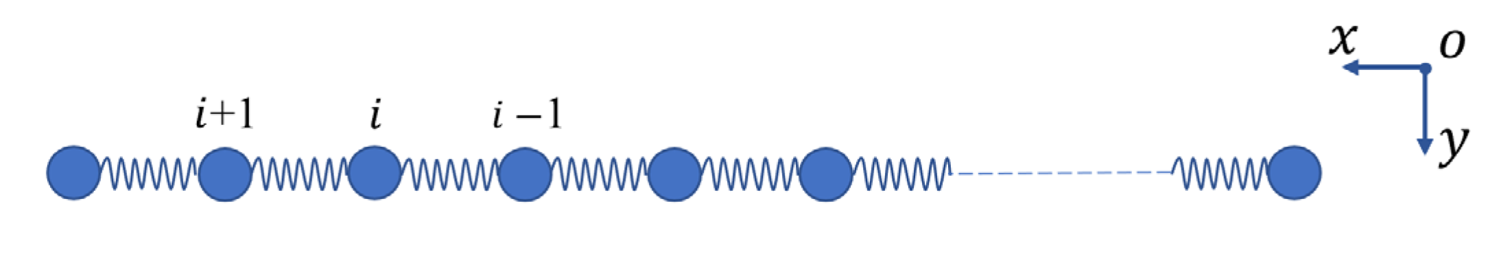
The cable state has a great impact on the dynamic performance of the wave glider system, and it will determine whether the float and glider are pulled by the cable. In the present work, the cable is discretized into several microelements to eliminate the impact of cable state on dynamic performance. Each element is treated as lumped masses which are connected with a massless spring (in Figure 6). This is a two-dimensional coordinate system, and each node of this simplified model is defined in the earth-fixed frame o x y [15].
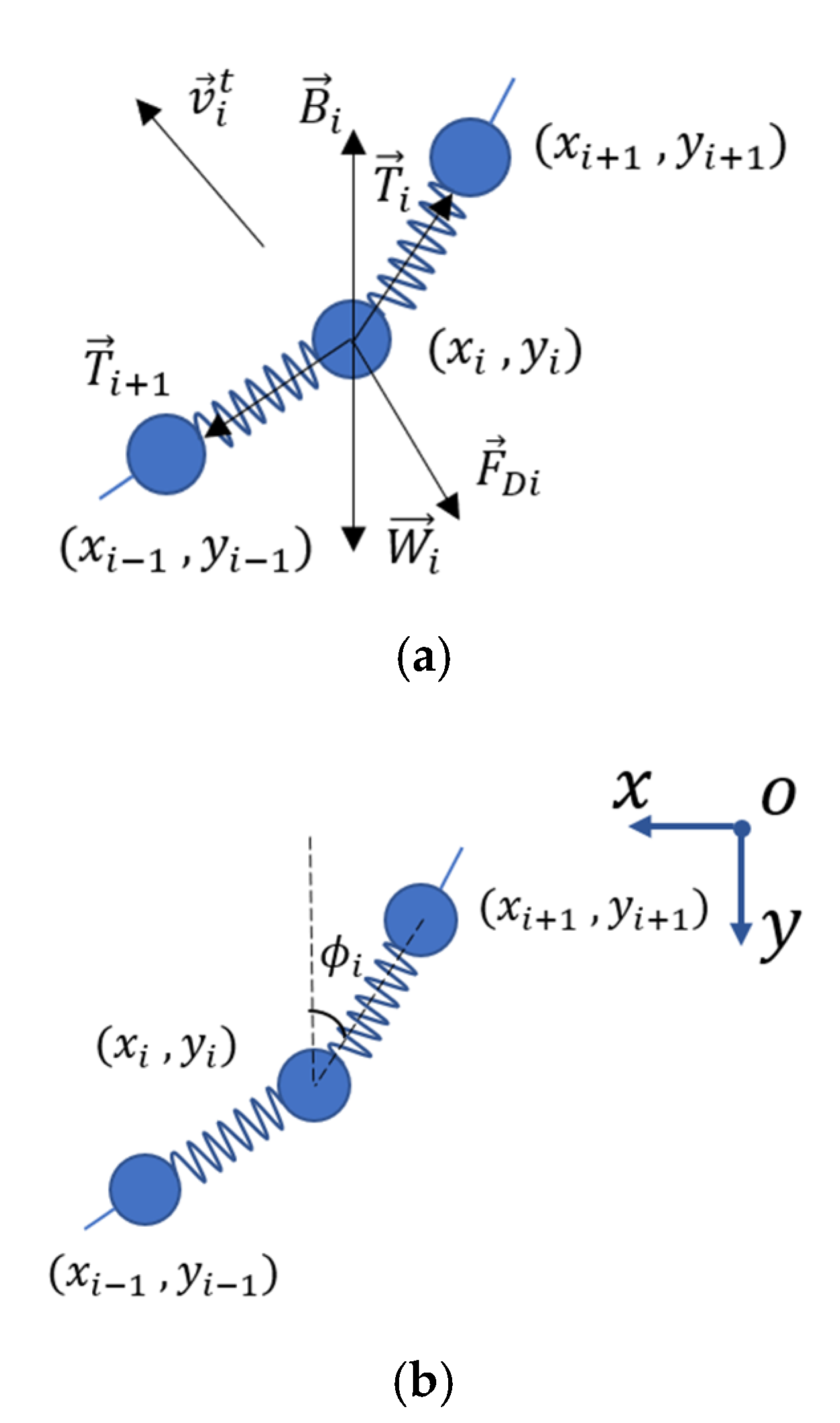
The forces acting on the cable respectively act on every single microelement during the deployment process. Force analysis of the cable is shown in Figure 7a, and the position of each node is shown in Figure 7b. Gravity ( G i t ), buoyancy ( F B i t ), tensile force ( T i ) and drag force ( F D i t ) are taken into consideration.
The 2D coupled model on node i is formulated as follows:
( m i t m i t ) ( ξ ¨ i t η ¨ i t ) = ( T i x + F D i x t T i y + F D i y t + G i t F B i t )
The cable model is established to express dynamic characteristics on a 2D plane, therefore, only transverse and longitudinal direction are considered. Where m i t is the node mass i , ξ i t and η i t are the node transverse and longitudinal displacement i , respectively.
T i is expressed as follows:
| T i 1 | = k i 1 ( l i 1 , i l i 1 , i )
| T i | = k i ( l i , i + 1 l i , i + 1 )
where k i is coefficient of tensile stiffness and its value depends on spring material. The value of k i can be expressed in a piecewise function:
k i = { k 0 l i , i + 1 > l i , i + 1 0 l i , i + 1 l i , i + 1
where l i , i + 1 is the initial length between node i and node i + 1 , l i , i + 1 is the length between node i , and node i + 1 is when the spring is under tension.
The transitive relation between two adjacent nodes can be written as follows:
T i x = T i sin ϕ i T i 1 sin ϕ i 1
T i y = T i cos ϕ i T i 1 cos ϕ i 1
The hinge joint approach is utilized to connect the float and glider by the cable. The float and glider are only subjected to unilateral tension force of the cable during the deployment process, and the components of tension forces on the glider are calculated as:
T 1 x = T 1 sin ϕ 1
T 1 y = T 1 cos ϕ 1
Similarly, the components of tension forces on the float are:
T n x = T n 1 sin ϕ n 1
T n y = T n 1 cos ϕ n 1
F D i x t and F D i y t are formulated as follows:
F D i x t = 1 2 C D ρ S x t ( v i x t ) 2 ( i )
F D i y t = 1 2 C D ρ S y t ( v i y t ) 2 ( j )
where S t is the cable immersed area, v i t is the mass point velocity at node i .
The cable gravity is kept constant during the deployment process, and the submerged cable volume is supposed to be unchangeable. They can be calculated by
G t = i = 1 n G i t
F B t = i = 1 n ρ g V i t

3. Simulation Analysis

The ocean environment is very complicated and varied in the real world. After considering the calculation cost and efficiency, the representative working condition with an amplitude of 0.2 m and the wave period of 3 s was selected as the deployment environment to investigate the dynamic performance. In this section, relative position of the float and glider is firstly presented. The effects of different deployment methods on velocities and tension force are respectively analyzed. The simulation performs in a 2D vertical plane. Hence, the inertia moment of the float and glider can be neglected. The main parameters of a wave glider system are shown in Table 1.

3.1. Displacement Analysis of the Wave Glider

The falling trajectory of a submerged glider and the forward moving trajectory of a float with different deployment methods are shown in Figure 8. The cable remains tense before laying in Figure 8a, and the float and glider are coincident. The float is dragged by the glider through a cable between them at 0 s. On the contrary, the cable is slack before laying in Figure 8b, and the mass center of the float as well as glider are almost coincident. The cable would be easily loosened when the glider falls faster than the float, and this process continues until the cable length is up to the maximum. The float has no horizontal displacement during this moment. Both of them will be stable after the fifth second. It is seen that Method 1 has a large displacement in 10 s, which is 7.3 m. On the contrary, Method 2 has a displacement of just 5.5 m at the same time. The trajectory after 5 s is not significantly different by comparing the two methods.
As we can see, Method 1 shows a larger displacement than Method 2; this may be because the float is dragged by the cable in all times for Method 1 and the wave energy can be fully utilized during this process. As for Method 2, the wave energy conversion efficiency is lower than Method 1 due to its deployment characteristics.

3.2. Velocity Analysis of the Wave Glider

In Figure 9, the fluctuation of velocity with respect to Method 1 and Method 2 is quite different within 5 s. The transverse velocity of the float using Method 1 reaches 2 m/s from 0 continuously as shown in Figure 9a, whereas Method 2 presents an abrupt change which reaches 3 m/s from 0, as shown in Figure 9b. The glider would accelerate without dragging the float for Method 2 in this process because the cable is slack before it reaches the limit length at 0–1.2 s. In addition, the change magnitude in float velocity is larger than the glider. The float and glider are decelerating after the peak velocity no matter what method is used. Then the velocity of the wave glider system fluctuates regularly. When the system is stable, the average velocity of the float and glider is the same for both Method 1 and Method 2, which is about 0.4 m/s.

3.3. Force Analysis of the Wave Glider during Process of Deployment

The tension forces of the hinged joint between cable and float were also calculated. The variations of tension forces over time for Method 1 and Method 2 are shown in Figure 10a,b, respectively. It can be seen that the maximum tension force increases from 500 N (Newton, International System of Units) (Method 1) to 1750 N (Method 2), which increases by 1250 N (up to 250%) because the time when the submerged glider provides active force for the system using Method 1 is earlier than that using Method 2. In the Method 2 deployment process, the cable is slack until the distance between the glider and the float is up to the cable length. In this process, the glider continues to accelerate until the cable is fully extended, then it will suddenly slow down due to the cable tension. Therefore, the cable will be under more tension in Method 2 than in Method 1.
Negative horizontal tension force appears at the time when the float is ahead of the glider (Figure 11a). Average horizontal tension force is not very different for both Method 1 and Method 2, which is about 5 N (Figure 11b). Figure 12 shows the hydrofoil thrust in the horizontal direction. As for Method 1, the force on hydrofoil presents a good continuity, whereas for Method 2 the force decreases suddenly at about 1.2 s.
It can be seen that the tension force is seriously sensitive to deployment methods. The cable tension of Method 1 is smaller due to its motion continuity. As a result, it is more beneficial to apply Method 1 into practice to improve the dynamic performance of the system and protect the structure.

4. Conclusions

In this paper, a 3-DOF dynamic model of a wave glider was established based on the multibody dynamic method. The dynamic characteristics of the deployment process were calculated by the numerical simulation method, and the dynamic responses of the wave glider were analyzed and compared under the different deployment methods. According to dynamic response, the following conclusions were drawn:
  • The displacement performance of two different methods was discussed. By analyzing deployment displacement curves, it can be seen that the wave glider system behaves unstably at the beginning of deployment, and then it tends to be stable after 5 s. Method 1 has a larger displacement than Method 2.
  • The velocity characteristics were obtained. Although the average velocity is not very different for each method, a sudden change of velocity will occur at 1.2 s when Method 2 is selected.
  • Deployment methods have quite an effect on tension force of the hinged joint between the cable and float. Method 2 suffers more serious tension than Method 1, which will lead to serious extra load on the structure of the wave glider. However, Method 1 performs more stably under the same conditions. Overall, Method 1 has smaller sudden impacts of the tension force and the best performance.
This paper investigated two different deployment methods which may provide a foundation for structural protection of the wave glider system. In the future, corresponding experimental testing should be carried out to further verify the numerical simulation in the present work.

Author Contributions

Conceptualization, Z.C.; investigation, G.L.; methodology, X.W., Z.C. and Z.Z.; software, X.W. and J.Z.; supervision, Z.C.; writing—original draft, X.W.; writing—review & editing, X.W., Z.C. and Z.F. All authors have read and agreed to the published version of the manuscript.

Funding

This research was funded by the National Natural Science Foundation of China, grant number 51875540; The Fundamental Research Funds for the Central Universities, grant number 201513053.

Conflicts of Interest

The authors declare no conflict of interest.

References

  1. Alaaeldeen, M.E.A.; Duan, W.Y. Overview on the development of autonomous underwater vehicles (AUVs). J. Ship Mech. 2016, 20, 768–787. [Google Scholar]
  2. Villareal, T.A.; Wilson, C. A comparison of the pac-X trans-pacific wave glider data and satellite data (MODIS, aquarius, TRMM and VIIRS). PLoS ONE 2014, 9. [Google Scholar] [CrossRef] [PubMed] [Green Version]
  3. Yang, F.M.; Shi, W.C.; Wang, D.Z. Systematic study on propulsive performance of tandem hydrofoils for a wave glider. Ocean Eng. 2019, 179, 361–370. [Google Scholar] [CrossRef] [Green Version]
  4. KRAUS, N.D. Wave glider dynamic modeling, parameter identification and simulation. Ph.D. Thesis, University of Hawaii, Honolulu, HI, USA, 2012. [Google Scholar]
  5. Caiti, A.; Calabró, V.; Grammatico, S.; Munafó, A.; Stifani, M. Lagrangian modeling of the underwater wave glider. In Proceedings of the OCEANS 2011 IEEE-Spain, Santander, Spain, 6–9 June 2011; 2011; pp. 1–6. [Google Scholar]
  6. Qi, Z.F.; Liu, W.X.; Jia, L.J.; Qin, Y.F.; Sun, X.J. Dynamic modeling and motion simulation for wave glider. Appl. Mech. Mater. 2013, 397, 285–290. [Google Scholar] [CrossRef]
  7. Zhou, C.L.; Wang, B.X.; Zhou, H.X.; Li, J.L.; Xiong, R. Dynamic modeling of a wave glider. Front. Inf. Technol. Electron. Eng. 2017, 18, 1295–1304. [Google Scholar] [CrossRef]
  8. Feng, Z.X.; Chang, Z.Y.; Zheng, Z.Q.; Wang, P.F. Effects of Connection Type between Surface Vessel and Submersible Propeller on Motion Performance of Wave Glider. Appl. Sci. 2018, 8, 2467. [Google Scholar] [CrossRef] [Green Version]
  9. Zhang, C.Y.; Xu, X.S. Research on Motion Relationship Between the Surface Boat and the Wave-Propelled Sub in Wave Glider System. J. Sichuan Ordnance 2018, 52, 127–132. [Google Scholar]
  10. Wang, L.F.; Li, Y.; Liao, Y.L.; Pan, K.W.; Zhang, W.X. Dynamics modeling of an unmanned wave glider with flexible umbilical. Ocean Eng. 2019, 180, 267–278. [Google Scholar] [CrossRef]
  11. Yang, F.M.; Shi, W.C.; Zhou, X.; Guo, B.; Wang, D.Z. Numerical investigation of a wave glider in head seas. Ocean Eng. 2018, 164, 127–138. [Google Scholar] [CrossRef] [Green Version]
  12. Shi, J.; Gong, W.; Qi, Z.F.; Jia, L.Y.; Zhang, F.; Qin, Y.F. Research of wave glider navigation control strategy based on multi-sensor. Transducer Microsyst. Technol. 2014, 33, 23–30. [Google Scholar]
  13. Wang, P.; Tian, X.L.; Lu, W.Y.; Hu, Z.H.; L, Y. Dynamic modeling and simulations of the wave glider. Appl. Math. Model. 2019, 66, 77–96. [Google Scholar] [CrossRef]
  14. Cong, B.; Cui, H.L.; Liu, Z. Modeling and Virtual Simulation in Random Ocean Waves. J. Xi’an Technol. Univ. 2009, 5. [Google Scholar]
  15. Wang, H.; Eberhard, P.; Lin, Z.Q. Modeling and simulation of closed loop multibody systems with bodies-joints composite modules. Multibody Syst. Dyn. 2010, 24, 389–411. [Google Scholar] [CrossRef]
Figure 1. A type of wave glider manufactured by Liquid Robotics Inc.
Jmse 08 00529 g001
Figure 2. Swimming with the wave glider.
Jmse 08 00529 g002
Figure 3. Working principle of the wave glider.
Jmse 08 00529 g003
Figure 4. Deployment method of wave glider (a) Method 1, (b) Method 2.
Jmse 08 00529 g004
Figure 5. Force analysis diagram of a wave glider.
Jmse 08 00529 g005
Figure 6. The simplified model of cable.
Jmse 08 00529 g006
Figure 7. (a) Force analysis on node i and (b) position of each nodes.
Jmse 08 00529 g007
Figure 8. Motion trajectory of a wave glider during the process of deployment of (a) Method 1 and (b) Method 2.
Jmse 08 00529 g008
Figure 9. Transverse velocities of float and glider (a) Method 1 and (b) Method 2.
Jmse 08 00529 g009aJmse 08 00529 g009b
Figure 10. Tension force of the hinged joint between cable and float (a) Method 1 and (b) Method 2.
Jmse 08 00529 g010aJmse 08 00529 g010b
Figure 11. Horizontal tension force to the hinged joint between cable and float: (a) comparison of Method 1 and Method 2; (b) enlarged force response curves.
Jmse 08 00529 g011
Figure 12. Hydrofoil thrust in horizontal direction.
Jmse 08 00529 g012
Table 1. Main parameters of a wave glider system.
ParametersValues
Mass of the float 41 kg
Mass of the glider50 kg
Float dimension 1.4   m × 0.52   m × 0.15   m
Underwater gravity of the glider 380 N
Area of hydrofoil600 cm2
Length of the cable2 m
Drag coefficients1.5
Spring stiffness106 N/m
Limit angle25°

