Experimental Validation and Comparison of Numerical Models for the Mooring System of a Floating Wave Energy Converter

 ,
,  , , ,
, , ,  ,
,  and
and 
Abstract
:1. Introduction
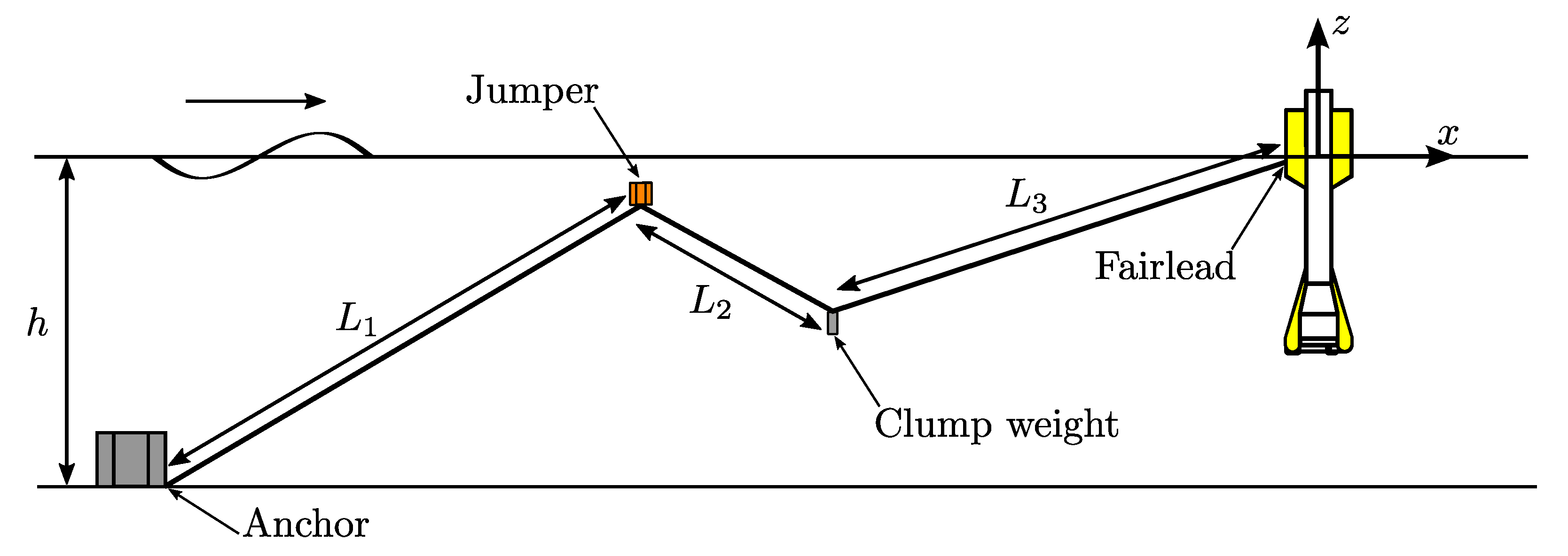
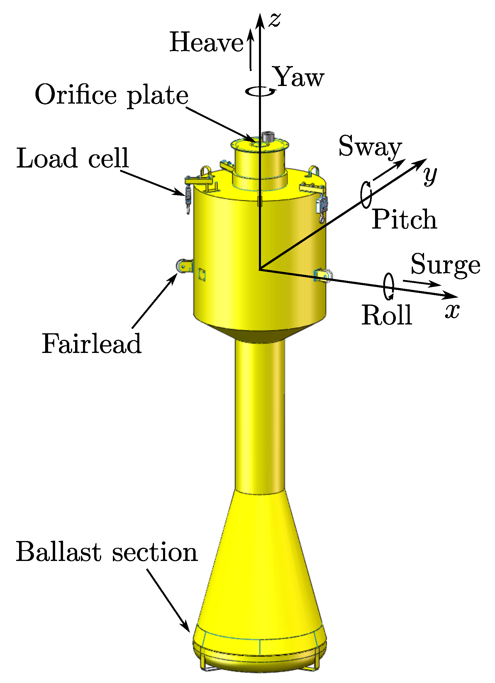
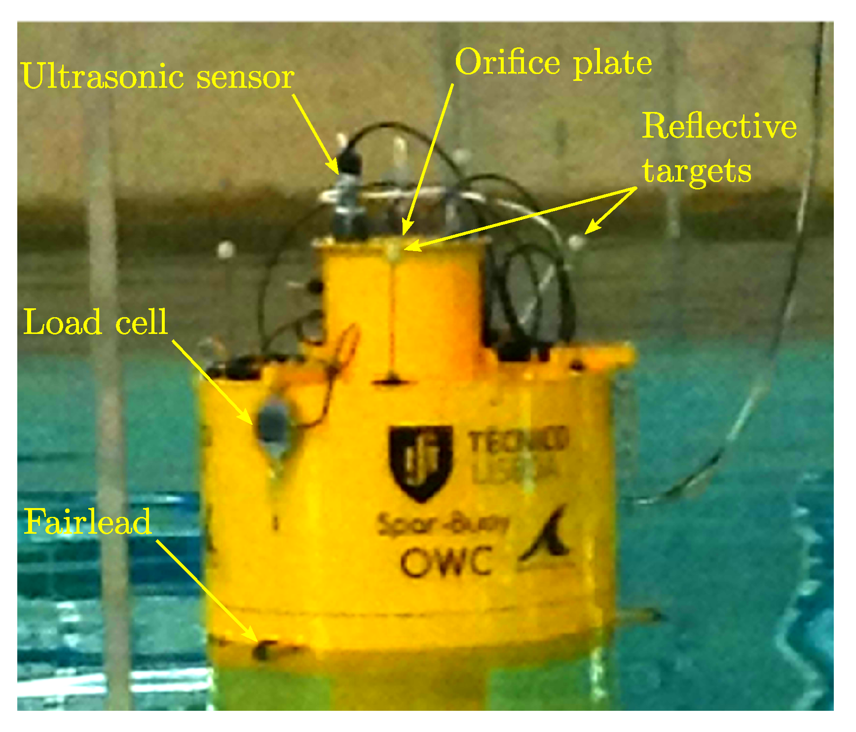
2. Experimental Set-Up
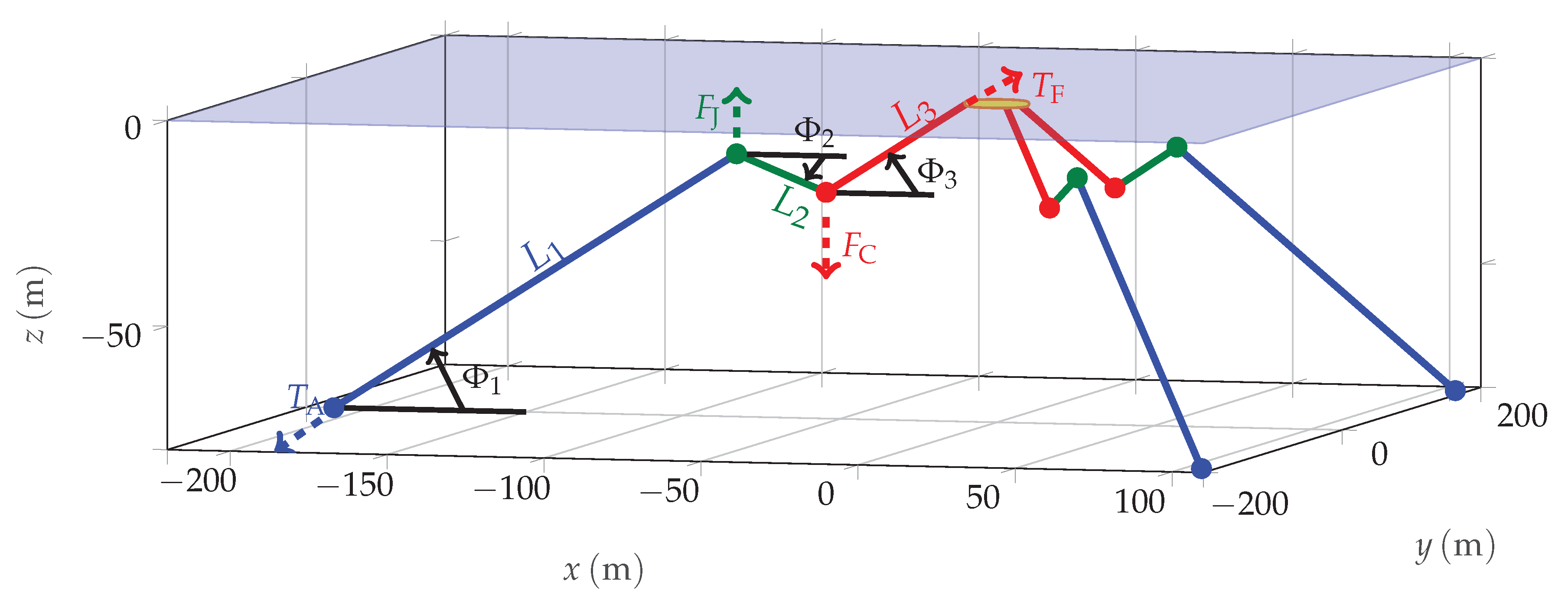
3. Mathematical Models of the Mooring System
3.1. QS Model
3.2. MoorDyn
- It creates a QS model that computes each node position, based on the provided input file.
- Then, dynamic relaxation is used to allow the system to settle to initial equilibrium, also including dynamic drag and acceleration forces.
- At each time step, MoorDyn calculates the tension at each fairlead and the motion (position, velocity and acceleration) of each node.
3.2.1. Input File
- Damping coefficient
- Bottom stiffness
3.2.2. QS Initial Phase
3.2.3. Dynamic Relaxation Phase
3.2.4. Simulation Phase
3.2.5. Scale
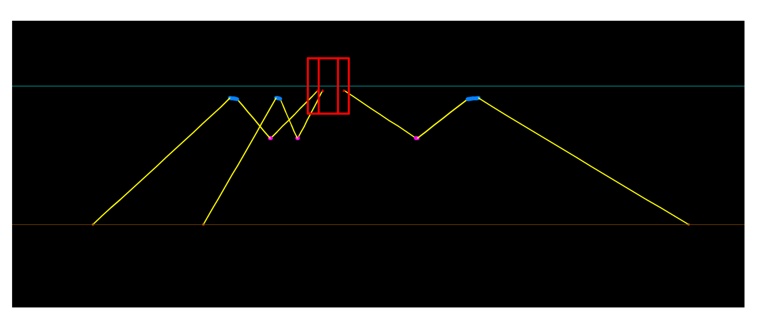
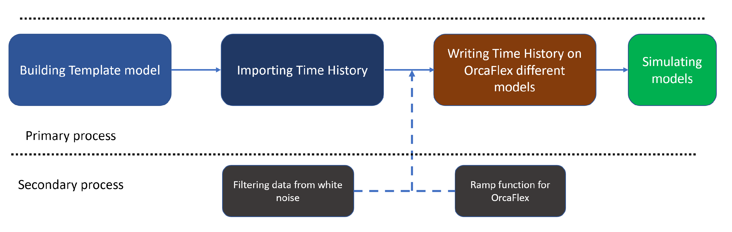
3.3. OrcaFlex
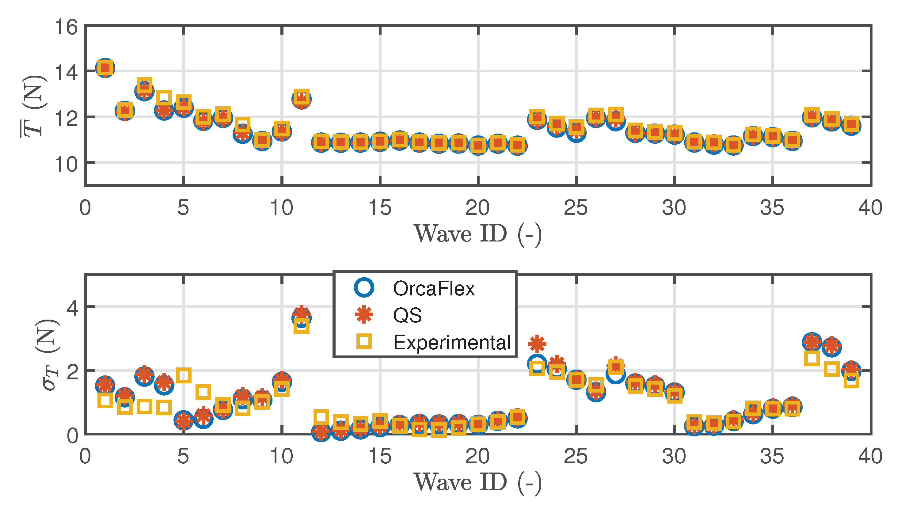
4. Comparison and Validation
5. Discussion
- Lines length (high sensitivity of the model).
- Lines stiffness (specially for taut, semi-taut mooring).
- Attachments properties (jumper and clump weight).
- Wave effects on mooring lines.
- Anchors position.
6. Conclusions
Author Contributions
Funding
Conflicts of Interest
References
- Astariz, S.; Iglesias, G. The economics of wave energy: A review. Renew. Sustain. Energy Rev. 2015, 45, 397–408. [Google Scholar] [CrossRef]
- McCombes, T.; Johnstone, C.; Holmes, B.; Myers, L.E.; Bahaj, A.; Heller, V.; Kofoed, J.; Finn, J.; Bittencourt, C. Assessment of Current Practice for Tank Testing of Small Marine Energy Devices; Technical Report; Aalborg University: Aalborg, Denmark, 2010. [Google Scholar]
- Ingram, D.; Smith, G.; Bittencourt-Ferreira, C.; Smith, H. Protocols for the Equitable Assessment of Marine Energy Converters; Technical Report; University of Edinburgh: Edinburgh, UK, 2011. [Google Scholar]
- Villate, J.L.; Ruiz-Minguela, P.; Berque, J.; Pirttimaa, L.; Cagney, D.; Cochrane, C.; Jeffrey, H. Strategic Research and Innovation Agenda for Ocean Energy; Technical Report; 2020; Available online: https://www.oceanenergy-europe.eu/wp-content/uploads/2020/05/ETIP-Ocean-SRIA.pdf (accessed on 27 July 2020).
- Kofoed, J.P.; Troch, P. Book of Abstracts. In Proceedings of the 2nd WECANet Annual Assembly, Porto, Portugal, 28–29 November 2019. [Google Scholar]
- Scotland, W.E. Cost Reduction in Supporting Infrastructure—Moorings and Foundations. 2018. Available online: https://library.waveenergyscotland.co.uk/other-activities/project-landscaping/phase-2/mooring-system/wes_ls06_er_moorings/ (accessed on 27 July 2020).
- Ma, K.T.; Luo, Y.; Kwan, T.; Wu, Y. Mooring design. In Mooring System Engineering for Offshore Structures; Elsevier: Amsterdam, The Netherlands, 2019; pp. 63–83. [Google Scholar] [CrossRef]
- DNV-OS-E301 Position Mooring. Available online: https://www.dnvgl.com/rules-standards/ (accessed on 24 July 2020).
- ISO. ISO 19901-7:2013—Petroleum and Natural Gas Industries—Specific Requirements for Offshore Structures—Part 7: Stationkeeping Systems for Floating Offshore Structures and Mobile Offshore Units. 2013. Available online: https://www.iso.org/standard/59298.html (accessed on 24 July 2020).
- Thomsen, J.B.; Ferri, F.; Kofoed, J.P.; Black, K. Cost optimisation of mooring solutions for large floating wave energy converters. Energies 2018, 11, 159. [Google Scholar] [CrossRef] [Green Version]
- Davidson, J.; Ringwood, J.V. Mathematical modelling of mooring systems for wave energy converters—A review. Energies 2017, 10, 666. [Google Scholar] [CrossRef] [Green Version]
- Giorgi, G.; Ringwood, J.V. Articulating parametric resonance for an OWC spar buoy in regular and irregular waves. J. Ocean Eng. Mar. Energy 2018, 4, 311–322. [Google Scholar] [CrossRef]
- Smith, R.J.; MacFarlane, C.J. Statics of a three component mooring line. Ocean Eng. 2001, 28, 899–914. [Google Scholar] [CrossRef]
- Bauduin, C.; Naciri, M. A contribution on quasi-static mooring line damping. J. Offshore Mech. Arct. Eng. ASME 2000, 122, 125–133. [Google Scholar] [CrossRef]
- Giorgi, G.; Gomes, R.P.F.; Bracco, G.; Mattiazzo, G. Numerical investigation of parametric resonance due to hydrodynamic coupling in a realistic wave energy converter. Nonlinear Dyn. 2020. [Google Scholar] [CrossRef]
- Wang, L.Z.; Guo, Z.; Yuan, F. Quasi-static three-dimensional analysis of suction anchor mooring system. Ocean Eng. 2010, 37, 1127–1138. [Google Scholar] [CrossRef]
- Nava, V.; Rajic, M.; Soares, C.G. Effects of the Mooring Line Configuration on the Dynamics of a Point Absorber. In Proceedings of the 32nd International Conference on Ocean, Offshore and Artic Engineering, Nantes, France, 9–14 June 2013. [Google Scholar]
- Aranha, J.A.; Pinto, M.O. Dynamic tension in risers and mooring lines: An algebraic approximation for harmonic excitation. App. Ocean Res. 2001, 23, 63–81. [Google Scholar] [CrossRef]
- Chai, Y.T.; Varyani, K.S.; Barltrop, N.D. Three-dimensional Lump-Mass formulation of a catenary riser with bending, torsion and irregular seabed interaction effect. Ocean Eng. 2002, 29, 1503–1525. [Google Scholar] [CrossRef]
- Chatjigeorgiou, I.K. A finite differences formulation for the linear and nonlinear dynamics of 2D catenary risers. Ocean Eng. 2008, 35, 616–636. [Google Scholar] [CrossRef]
- Montano, A.; Restelli, M.; Sacco, R. Numerical simulation of tethered buoy dynamics using mixed finite elements. Comput. Methods Appl. Mech. Eng. 2007, 196, 4117–4129. [Google Scholar] [CrossRef]
- ANSYS. Aqwa Theory Manual. 2013. Available online: https://cyberships.files.wordpress.com/2014/01/wb_aqwa.pdf (accessed on 8 May 2012).
- Orcina. OrcaFlex—Documentation, 10.1b Edition. 2020. Available online: https://www.orcina.com/releases/orcaflex-101/ (accessed on 24 July 2020).
- Hall, M. MoorDyn User’s Guide. 2015. Available online: http://www.matt-hall.ca/ (accessed on 24 July 2020).
- Palm, J. Mooring Dynamics for Wave Energy Applications. Ph.D. Thesis, Chalmers University of Technology, Gothenburg, Sweden, 2017. [Google Scholar]
- Harnois, V.; Weller, S.D.; Johanning, L.; Thies, P.R.; Le Boulluec, M.; Le Roux, D.; Soulé, V.; Ohana, J. Numerical model validation for mooring systems: Method and application for wave energy converters. Renew. Energy 2015, 75, 869–887. [Google Scholar] [CrossRef] [Green Version]
- Yang, S.H.; Ringsberg, J.W.; Johnson, E.; Hu, Z.Q.; Palm, J. A comparison of coupled and de-coupled simulation procedures for the fatigue analysis of wave energy converter mooring lines. Ocean Eng. 2016, 117, 332–345. [Google Scholar] [CrossRef] [Green Version]
- Palm, J.; Eskilsson, C.; Paredes, G.M.; Bergdahl, L. Coupled mooring analysis for floating wave energy converters using CFD: Formulation and validation. Int. J. Mar. Energy 2016, 16, 83–99. [Google Scholar] [CrossRef] [Green Version]
- Bhinder, M.A.; Karimirad, M.; Weller, S.; Debruyne, Y.; Guérinel, M.; Sheng, W. Modelling mooring line non-linearities (material and geometric effects) for a wave energy converter using AQWA, SIMA and Orcaflex. In Proceedings of the 11th European Wave and Tidal Energy Conference, Nantes, France, 6–11 September 2015; pp. 1–10. [Google Scholar]
- Vissio, G.; Passione, B.; Hall, M.; Raffero, M. Expanding ISWEC Modelling with a Lumped-Mass Mooring Line Model. In Proceedings of the 11th European Wave and Tidal Energy Conference, Nantes, France, 6–11 September 2015; pp. 1–9. [Google Scholar]
- Giorgi, G.; Gomes, R.P.; Henriques, J.C.; Gato, L.M.; Bracco, G.; Mattiazzo, G. Detecting parametric resonance in a floating oscillating water column device for wave energy conversion: Numerical simulations and validation with physical model tests. Appl. Energy 2020, 276. [Google Scholar] [CrossRef]
- Hall, M.; Goupee, A. Validation of a lumped-mass mooring line model with DeepCwind semisubmersible model test data. Ocean Eng. 2015, 104, 590–603. [Google Scholar] [CrossRef] [Green Version]
- Gomes, R.P.; Henriques, J.C.; Gato, L.M.; Falcão, A.F. Wave power extraction of a heaving floating oscillating water column in a wave channel. Renew. Energy 2016, 99, 1262–1275. [Google Scholar] [CrossRef]
- Correia da Fonseca, F.; Gomes, R.; Henriques, J.; Gato, L.; Falcão, A. Model testing of an oscillating water column spar-buoy wave energy converter isolated and in array: Motions and mooring forces. Energy 2016, 112, 1207–1218. [Google Scholar] [CrossRef]
- Bracco, G.; Casassa, M.; Giorcelli, E.; Giorgi, G.; Martini, M.; Mattiazzo, G.; Passione, B.; Raffero, M.; Vissio, G. Application of sub-optimal control techniques to a gyroscopic Wave Energy Converter. In Renewable Energies Offshore; Taylor & Francis Group: London, UK, 2014; pp. 265–269. [Google Scholar]
- Sirigu, S.A.; Bonfanti, M.; Begovic, E.; Bertorello, C.; Dafnakis, P.; Giorgi, G.; Bracco, G.; Mattiazzo, G. Experimental Investigation of Mooring System on a Wave Energy Converter in Operating and Extreme Wave Conditions. J. Mar. Sci. Eng. 2020, 8, 180. [Google Scholar] [CrossRef] [Green Version]
- Moura Paredes, G.; Palm, J.; Eskilsson, C.; Bergdahl, L.; Taveira-Pinto, F. Experimental investigation of mooring configurations for wave energy converters. Int. J. Mar. Energy 2016, 15, 56–67. [Google Scholar] [CrossRef]
- Giorgi, G.; Davidson, J.; Habib, G.; Bracco, G.; Mattiazzo, G.; Kalmár-nagy, T. Nonlinear Dynamic and Kinematic Model of a Spar-Buoy: Parametric Resonance and Yaw Numerical Instability. J. Mar. Sci. Eng. 2020, 8, 504. [Google Scholar] [CrossRef]
- Wendt, F.; Nielsen, K.; Yu, Y.H.; Bingham, H.; Eskilsson, C.; Kramer, B.; Babarit, A.; Bunnik, T.; Costello, R.; Crowley, S.; et al. Ocean Energy Systems wave energy modeling task: Modeling, verification, and validation of wave energy converters. J. Mar. Sci. Eng. 2019, 7, 379. [Google Scholar] [CrossRef] [Green Version]
- Ransley, E.; Yan, S.; Brown, S.; Graham, D.; Musiedlak, P.H.; Windt, C.; Ringwood, J.; Davidson, J.; Schmitt, P.; Wang, J.X.H.; et al. A blind comparative study of focused wave interactions with floating structures ({CCP-WSI Blind Test Series 3}). Int. J. Offshore Pol. Eng. 2020, 30, 1–10. [Google Scholar] [CrossRef] [Green Version]
- Giorgi, G.; Ringwood, J.V. Parametric motion detection for an oscillating water column spar buoy. In Proceedings of the 3rd International Conference on Renewable Energies Offshore RENEW, Lisbon, Portugal, 8–10 October 2018. [Google Scholar]
- Giorgi, G.; Ringwood, J.V. Articulating parametric nonlinearities in computationally efficient hydrodynamic models. In Proceedings of the 11th IFAC Conference on Control Applications in Marine Systems, Robotics, and Vehicles, Opatija, Croatia, 10–12 September 2018. [Google Scholar]
- Fontana, M.; Casalone, P.; Sirigu, S.A.; Giorgi, G. Viscous Damping Identification for a Wave Energy Converter Using CFD-URANS Simulations. J. Mar. Sci. Eng. 2020, 8, 355. [Google Scholar] [CrossRef]
- Sirigu, A.S.; Gallizio, F.; Giorgi, G.; Bonfanti, M.; Bracco, G.; Mattiazzo, G. Numerical and Experimental Identification of the Aerodynamic Power Losses of the ISWEC. J. Mar. Sci. Eng. 2020, 8, 49. [Google Scholar] [CrossRef] [Green Version]
- Genuardi, L.; Bracco, G.; Sirigu, S.A.; Bonfanti, M.; Paduano, B.; Dafnakis, P.; Mattiazzo, G. An application of model predictive control logic to inertial sea wave energy converter. In Mechanisms and Machine Science; Springer: Delft, The Netherland, 2019; Volume 73, pp. 3561–3571. [Google Scholar] [CrossRef]
- Bonfanti, M.; Bracco, G.; Dafnakis, P.; Giorcelli, E.; Passione, B.; Pozzi, N.; Sirigu, S.; Mattiazzo, G. Application of a passive control technique to the ISWEC: Experimental tests on a 1:8 test rig. In Proceedings of the NAV International Conference on Ship and Shipping Research, Trieste, Italy, 20–22 June 2018; Number 221499, pp. 60–70. [Google Scholar] [CrossRef]
- Masciola, M.; Robertson, A.; Jonkman, J.; Driscoll, F. Investigation of a FASTOrcaFlex Coupling Module for Integrating Turbine and Mooring Dynamics of Offshore Floating Wind Turbines. In Proceedings of the International Conference on Offshore Wind Energy and Ocean Energy, Rotterdam, The Netherlands, 2011. [Google Scholar]
- Wendt, F.; Robertson, A.; Jonkman, J.; Andersen, M.T. Verification and Validation of the New Dynamic Mooring Modules Available in FAST v8. In Proceedings of the International Ocean and Polar Engineering Conference (ISOPE), Rhodes, Greece, 26 June–1 July 2016. [Google Scholar]
- Gomes, R.P.F.; Henriques, J.C.; Gato, L.M.C.; Falcão, A.F. Hydrodynamic optimisation of an axisymmetric floating oscillating water column for wave energy conversion. Renew. Energy 2012, 44, 328–339. [Google Scholar] [CrossRef]
- Pozzi, N.; Bracco, G.; Passione, B.; Sirigu, S.A.; Mattiazzo, G. PeWEC: Experimental validation of wave to PTO numerical model. Ocean Eng. 2018, 167, 114–129. [Google Scholar] [CrossRef]
- Sirigu, S.A.; Bonfanti, M.; Passione, B.; Begovic, E.; Bertorello, C.; Dafnakis, P.; Bracco, G.; Giorcelli, E.; Mattiazzo, G. Experimental investigation of the hydrodynamic performance of the ISWEC 1:20 scaled device. In Proceedings of the NAV International Conference on Ship and Shipping Research (Number 221499), Trieste, Italy, 20–22 June 2018; pp. 551–560. [Google Scholar] [CrossRef]
- Giorgi, G.; Gomes, R.P.F.; Bracco, G.; Mattiazzo, G. The effect of mooring line parameters in inducing parametric resonance on the Spar-buoy oscillating water column wave energy converter. J. Mar. Sci. Eng. 2020, 8, 29. [Google Scholar] [CrossRef] [Green Version]
- Vicente, P.C.; Falcão, A.F.O.; Justino, P.A.P. Non-linear Slack-Mooring Modelling of a Floating Two-Body Wave Energy Converter. In Proceedings of the 9th European Wave and Tidal Energy Conference, Southampton, UK, 5–9 September 2011. [Google Scholar]
- Journee, J.M.J.; Massie, W.W. Offshore Hydromechanics, 1st ed.; Delft University of Technology: Delft, The Netherland, 2001. [Google Scholar]
- Thomsen, J.B.; Ferri, F.; Kofoed, J.P. Screening of available tools for dynamic mooring analysis of wave energy converters. Energies 2017, 10, 853. [Google Scholar] [CrossRef] [Green Version]
- MooDy User’s Manual—Mooring Dynamics. Available online: https://github.com/johannep/moodyAPI (accessed on 24 July 2020).
- ProteusDS Manual—DSA. Available online: https://prometheus.io/docs/ (accessed on 24 July 2020).
- Fackrell, S. Scholarship at UWindsor Scholarship at UWindsor Study of the Added Mass of Cylinders and Spheres Study of the Added Mass of Cylinders and Spheres. Ph.D. Thesis, University of Windsor, Windsor, ON, Canada, 2011. [Google Scholar]
- Paredes, G.M. Study of Mooring Systems for Offshore Wave Energy Converters. Ph.D. Thesis, Faculdade de Engenharia da Universidade do Porto, Porto, Portugal, 2016. [Google Scholar]


| Regular Waves | Irregular Waves | ||||
|---|---|---|---|---|---|
| Wave ID | (s) | (cm) | Wave ID | (s) | (cm) |
| 1 | 1.6 | 16.2 | 23 | 1.8 | 15.3 |
| 2 | 1.8 | 15.9 | 24 | 2.4 | 14.8 |
| 3 | 2.0 | 15.2 | 25 | 2.5 | 14.0 |
| 4 | 2.2 | 15.5 | 26 | 1.3 | 14.4 |
| 5 | 1.0 | 11.4 | 27 | 1.8 | 15.1 |
| 6 | 1.2 | 11.7 | 28 | 3.7 | 15.1 |
| 7 | 1.4 | 17.1 | 29 | 3.7 | 14.8 |
| 8 | 2.4 | 16.5 | 30 | 3.8 | 14.5 |
| 9 | 2.6 | 13.1 | 31 | 1.8 | 4.4 |
| 10 | 2.8 | 11.3 | 32 | 2.2 | 4.5 |
| 11 | 3.0 | 13.2 | 33 | 3.6 | 4.4 |
| 12 | 1.0 | 4.4 | 34 | 1.8 | 9.0 |
| 13 | 1.2 | 3.3 | 35 | 2.5 | 8.9 |
| 14 | 1.4 | 4.8 | 36 | 3.6 | 8.9 |
| 15 | 1.6 | 4.7 | 37 | 2.5 | 14.7 |
| 16 | 1.8 | 4.5 | 38 | 2.2 | 14.7 |
| 17 | 2.0 | 4.3 | 39 | 3.5 | 15.0 |
| 18 | 2.2 | 4.7 | |||
| 19 | 2.4 | 4.6 | |||
| 20 | 2.6 | 4.2 | |||
| 21 | 2.8 | 2.8 | |||
| 22 | 3.0 | 4.2 | |||
| Parameter | Small-Scale (1:32) | Full-Scale |
|---|---|---|
| Buoy diameter, (m) | ||
| OWC diameter, (m) | ||
| Total length (m) | ||
| Floater section draft (m) | ||
| Buoy draft, (m) | ||
| z-coordinate of CoB, (m) | ||
| z-coordinate of CoG, (m) | ||
| Metacentric height, (m) | ||
| Displaced volume, V (m) | ||
| Buoy mass, m (kg) |
| Parameter | Model-Scale (1:32) | Full-Scale |
|---|---|---|
| Line diameter, (mm) | 1 | 32 |
| Net line linear density, (kg m) | 0.03 | 34.82 |
| Jumper mass, (kg) | 0.12 | 4030.46 |
| Jumper density, (kg m) | 123.00 | 123.00 |
| Clump-weight mass, (kg) | 1.10 | 36,139.83 |
| Clump-weight density, (kg m) | 8097.50 | 8097.50 |
| Length of line anchor-jumper, (m) | 4.48 | 143.28 |
| Length of line jumper-clump-weight, (m) | 1.16 | 37.01 |
| Length of line fairlead-clump-weight, (m) | 1.58 | 50.40 |
| Anchor radius, (m) | 6.60 | 211.2 |
| Anchor z-coordinate, (m) | −2.50 | −80 |
| Fairlead radial coordinate, (m) | −0.29 | −9.28 |
| Fairlead z-coordinate, (m) | −0.08 | −2.58 |
| Software | Commercial Developer |
|---|---|
| Aqwa | ANSYS |
| OrcaFlex | Orcina |
| SESAM | DNV-GL |
| MoorDyn | - |
| Moody | - |
| Software | Type | Parallelization | Relative Computational Time s/s |
|---|---|---|---|
| OrcaFlex | Dynamic | yes | |
| MoorDyn | Dynamic | no | |
| In-house | Quasi-static | yes |
| Modes | Frequency (Hz) |
|---|---|
| Mode 1 | 0.3293 |
| Mode 2 | 0.32952 |
| Mode 3 | 0.32952 |
| Mode 4 | 0.35074 |
| Mode 5 | 0.35095 |
| Mode 6 | 0.35096 |
| Mode 7 | 0.63901 |
| ... | ... |
© 2020 by the authors. Licensee MDPI, Basel, Switzerland. This article is an open access article distributed under the terms and conditions of the Creative Commons Attribution (CC BY) license (http://creativecommons.org/licenses/by/4.0/).
Share and Cite
Paduano, B.; Giorgi, G.; Gomes, R.P.F.; Pasta, E.; Henriques, J.C.C.; Gato, L.M.C.; Mattiazzo, G. Experimental Validation and Comparison of Numerical Models for the Mooring System of a Floating Wave Energy Converter. J. Mar. Sci. Eng. 2020, 8, 565. https://doi.org/10.3390/jmse8080565
Paduano B, Giorgi G, Gomes RPF, Pasta E, Henriques JCC, Gato LMC, Mattiazzo G. Experimental Validation and Comparison of Numerical Models for the Mooring System of a Floating Wave Energy Converter. Journal of Marine Science and Engineering. 2020; 8(8):565. https://doi.org/10.3390/jmse8080565
Chicago/Turabian StylePaduano, Bruno, Giuseppe Giorgi, Rui P. F. Gomes, Edoardo Pasta, João C. C. Henriques, Luís M. C. Gato, and Giuliana Mattiazzo. 2020. "Experimental Validation and Comparison of Numerical Models for the Mooring System of a Floating Wave Energy Converter" Journal of Marine Science and Engineering 8, no. 8: 565. https://doi.org/10.3390/jmse8080565
APA StylePaduano, B., Giorgi, G., Gomes, R. P. F., Pasta, E., Henriques, J. C. C., Gato, L. M. C., & Mattiazzo, G. (2020). Experimental Validation and Comparison of Numerical Models for the Mooring System of a Floating Wave Energy Converter. Journal of Marine Science and Engineering, 8(8), 565. https://doi.org/10.3390/jmse8080565