Article

Wave Orbital Velocity Effects on Radar Doppler Altimeter for Sea Monitoring

by
Ferdinando Reale
*,
Eugenio Pugliese Carratelli
,
Angela Di Leo
and
Fabio Dentale
Department of Civil Engineering, University of Salerno, 84084 Fisciano, Italy
*
Author to whom correspondence should be addressed.
J. Mar. Sci. Eng. 2020, 8(6), 447; https://doi.org/10.3390/jmse8060447
Submission received: 22 May 2020 / Revised: 11 June 2020 / Accepted: 14 June 2020 / Published: 19 June 2020
(This article belongs to the Special Issue Radar Technology for Coastal Areas and Open Sea Monitoring)

Abstract

:
The orbital velocity of sea wave particles affects the value of sea surface parameters as measured by radar Doppler altimeters (also known as delay Doppler altimeter (DDA)). In DDA systems, the along-track resolution is attained by algorithms that take into account the Doppler shift induced by the component along the Earth/antenna direction of the satellite velocity, VS. Since the vertical component of the wave particle orbital velocity also induces an additional Doppler effect (in the following R-effect), an error arises on the positioning of the target on the sea surface. A numerical investigation shows that when the wavelength of sea waves is of the same order of magnitude of the altimeter resolution, the shape of the waveform might be significantly influenced by the R-effect. The phenomenon can be particularly important for the monitoring of long swells, such as those that often take place in the oceans.

1. Introduction

Radar altimetry is a widely acknowledged and largely diffused tool for open sea monitoring. Its basic principles are well known, and need not be described here, since they have been the object of extensive literature [1,2,3].
Conventional radar altimeters (low resolution mode (LRM)), with their along-track resolution on the order of a few kilometres, have indeed proven to be essential in monitoring sea parameters such as significant wave height (SWH) and sea surface height (SSH) from satellites such as ERS-1, ERS-2, Envisat, Jason-1, etc. They have thus become an essential tool in ocean forecasting, climate analysis, and sea level monitoring [4].
Recent developments have led to a widespread adoption of radar Doppler altimeters (also known as delay Doppler altimeter (DDA)), which provide a much higher along-track resolution (on the order of a few hundred metres); while this potentially improves the possibility of monitoring the ocean parameters, it also enhances some problems related to sea surface data analysis.
Over the years, a number of difficulties have indeed arisen in assessing how various physical effects may impact the reliability of the measurements. For instance, a well-known problem—common to both conventional and Doppler altimetry—is the so-called electromagnetic bias [5], through which the SWH influences the SSH; also, the presence of foam on the sea surface may influence both SWH and SSH measurements [6,7].
The possible influence of sea state on the oscillation of measured SSH was investigated by different authors [8,9,10], who showed that 10 Hz root mean square SSH is statistically linked to the value of SWH itself.
An aspect that recently was shown to be of considerable importance for DDA is the influence of very long waves upon the monitoring of SWH and SSH; the along-track resolution of DDA is indeed on the same order of, or even lower than, wavelength of the ocean swell.
Moreau et al. [11,12,13] compared eight months of CryoSat-2 data over long ocean swell and found that, on the one hand, the waveforms derived from DDA are dissimilar from those obtained through conventional altimetry, and on the other hand, the shape of such waveforms is considerably different from the usual shape. By investigating such shapes, they found that sometimes—but not always—the presence of swell is highlighted by a double peak in DDA measurements (Figure 1). It is worth noting that most SWH retrieving algorithms assume a Gaussian distribution of the instantaneous water height—which is not true in a swell dominated sea.
These results raise concerns about the potential impact of such ocean wave effects on the monitoring of sea state conditions.
The present paper deals with a related problem, i.e., the interference of wave orbital velocity on the DDA algorithm. Such an effect, first reported in 2016 by Reale et al. [14,15,16], was recently (2019) also tackled in [17,18,19,20]. In the following, after a brief recall of the principles of DDA, a numerical procedure is implemented to show the influence of such an effect on the DDA response, and, where possible, to confirm its presence on the basis of published results.

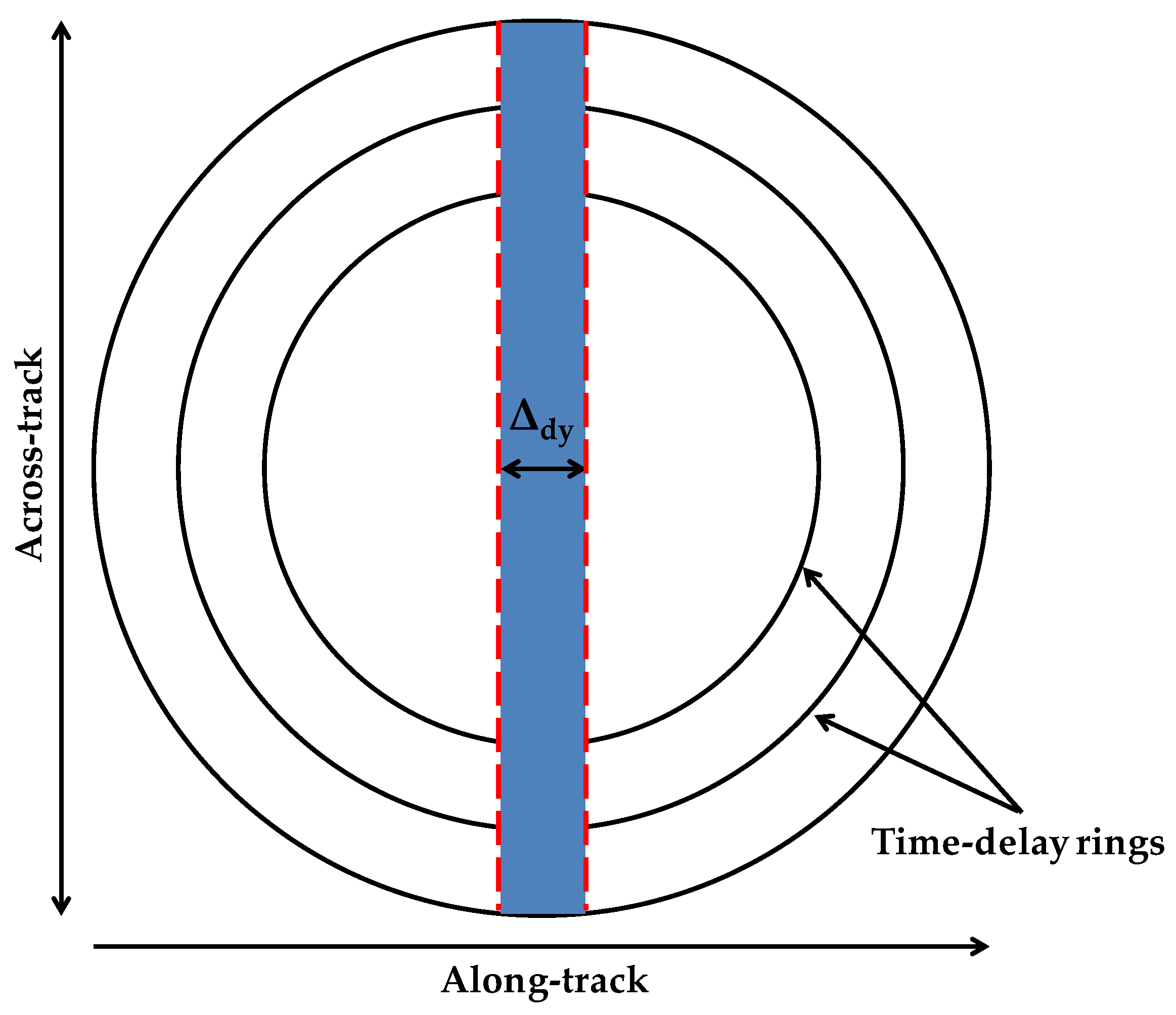
2. Materials and Methods

DDA is similar in concept to conventional radar altimetry, in that a power/time curve (in the following: “waveform”) of a reflected radio wave pulse is produced, and by analyzing such a curve, an accurate monitoring can be carried out of both SSH and SWH. In order to clarify the subject of the present paper, it is necessary to briefly recall main principles of DDA and its basic definitions, according to current literature [21,22,23,24].
DDA provides a decisive improvement of the resolution along the direction of the flight track (also known as along-track or azimuth direction) by taking into account the Doppler shift caused by the relative velocity of the satellite—or aircraft—borne antenna. The waveform is formed, in the same way as in conventional altimetry, by the variation in time of the illuminated sea surface (see Figure 2), but in DDA, the return signal is split into Δdy wide strips perpendicular to the along-track direction Y.
The resolution along the Y direction is given by the Doppler shift resolution fres, i.e., by the accuracy with which the altimeter can separate the return beam frequencies. Following [21,22], the Doppler frequency fd and the distance along Y from the Nadir are linked by the following two equations:
f d = 2 V S λ Y h ,
Y = λ h 2 V S f d ,
where Vs is the Earth/satellite relative velocity, h is the distance from the ground to the antenna, and λ is the electromagnetic wavelength. It is easy to see that the effect is governed by the projection Vc of Vs along the connection from the sea surface to the antenna, which can be taken to be approximately equal to VSY/h. A point (or a surface element on the sea) gives a contribution to the reflected intensity (and is therefore considered in the measurement procedure) only if its Doppler shift frequency fd is comprised between fres/2 and −fres/2, and therefore its velocity component Vc is comprised between VsΔdy/(2h) and −VsΔdy/(2h), Δdy being the nominal width of the resolution along Y (see Figure 3).
We have thus:
Δ d y = λ h f r e s 2 V S .
In a typical DDA altimeter, the footprint corresponds to an elongated strip on the surface, with an across-track resolution of 5–6 km and an along-track resolution of around 300 m. In presence of waves, the water surface is not still, and each water particle is affected—among others—by a vertical orbital velocity component VZ; such a component algebraically adds to the Vc velocity due to the antenna relative movement, thus introducing a further Doppler shift fR, indicated in the following as “R-effect” [14,16].
It is worth noting that a similar disturbance effect, sometimes known as “velocity bunching”, on imaging SAR radars has been discovered as far back as in the 1980s [25], and has been considered and studied ever since [26]. It constitutes a limit to the applications of SAR, but it was recently found that it can been used to extract further information about the wind and the sea state (cut-off effect, [27,28]).
Since the radial direction from the water surface to the antenna is nearly vertical, fR is given by following Equation (4) (Figure 4):
f R = 2 V Z λ .
The nearly vertical apparent velocity of a water particle with respect to the antenna is therefore VC+VSY/h, and its total Doppler frequency shift ft is given by Equation (5):
f t = f d + f R = 2 V S Y λ h + 2 V Z λ = 2 λ ( V S Y h + V Z ) .
If ft for a given point (red point in Figure 4) is greater than fres /2 or less than −fres/2, the point will be not taken into account, and the value of its instantaneous elevation η will not be considered by the algorithms, even if its geometrical position (position 1 in Figure 4) is located within the nominal width Δdy; conversely, a point located outside the nominal position (green point in Figure 4) will appear, due to the R-effect, to be located inside (position 2’ in Figure 4), and will be considered in all the statistics.
It is easy to see that a potential bias does exist, and it has to be evaluated; it remains to be seen whether the phenomenon is significant enough, i.e., if the order of magnitude of the R-effect is the same as that of the Vs induced Doppler, and if the error averages out in practical application.
Considering, for instance, the parameters of the CryoSat-2 satellite operating in SAR mode (see Table 1), and assuming, e.g., a 2 meter-high sinusoidal 225 meter-long wave in deep water (T ≈ 12 s), the vertical orbital velocity component VZ varies between −0.52 m/s and +0.52 m/s, while for a shorter and higher wave (H = 4 m; L = 125 m; T ≈ 9 s) the effect is more important (VZ varies between −1.41 m/s and +1.41 m/s).
Figure 5 shows, graphically, some comparisons between the orbital velocity induced Doppler frequency shift fR and the satellite velocity Doppler effect fd.
A more accurate assessment is thus necessary, and some numerical experiments described in the next paragraph help clarify the issue.

3. Simulation and Results

The consequences of R-effect on DDA measurement can only be assessed numerically; for this work, a conceptual model was used for the reconstruction of sea surface height from DDA. The examples provided here are relative to the CryoSat-2 satellite altimeter, with the parameters as reported in Table 1 above.
A computational procedure was thus implemented on an XY grid, whose side Lx is equal to the across-track resolution, and Ly is sufficiently long to include all the points whose apparent positions are located within the along-track resolution Δdy. The computational steps are called DX and DY, respectively.
The sea water instantaneous height η(X,Y), as well as its vertical velocity component VZ(X,Y), was computed on all the points in the grid. With reference to Figure 4, the Doppler frequency shift ft of a given point is given by Equation (5), so that its apparent position Yai is:
Y a i = Y i + ( f R + f d ) λ h 2 V S .
The strip will thus belong, or not, to the Doppler resolution strip Δdy, according to whether Δdy/2 < Yai < Δdy/2 or not.
The influence of wave induced Doppler shift can be first observed by considering the formation of waveforms; as stated above, R-effect changes the apparent position of reflected spots of the sea surface, so that the effective borders of the resolution zone are no longer simply given by Equation (2); this in turn will affect the waveform shape. In order to investigate this aspect, the points on the sea geometrically positioned in and around the nominal beam Δdy were relocated by taking the R-effect into account. By numerical computation, the distribution of distances between the antenna and the instantaneous simulated waveform (in the following: WF) can thus be constructed. This algorithm is simplified, since it neglects purely electromagnetic (e/m) effects, such as the antenna miss-pointing and the measurements noise, and it does not take into accounts the effects of the curvature of the Earth; it is therefore only meant to verify the effect that is being discussed here, which is purely geometrical and hydrodynamical.
The procedure was repeated twice, once by activating the R-effect, and once by ignoring it so that the simulated waveforms could be compared.

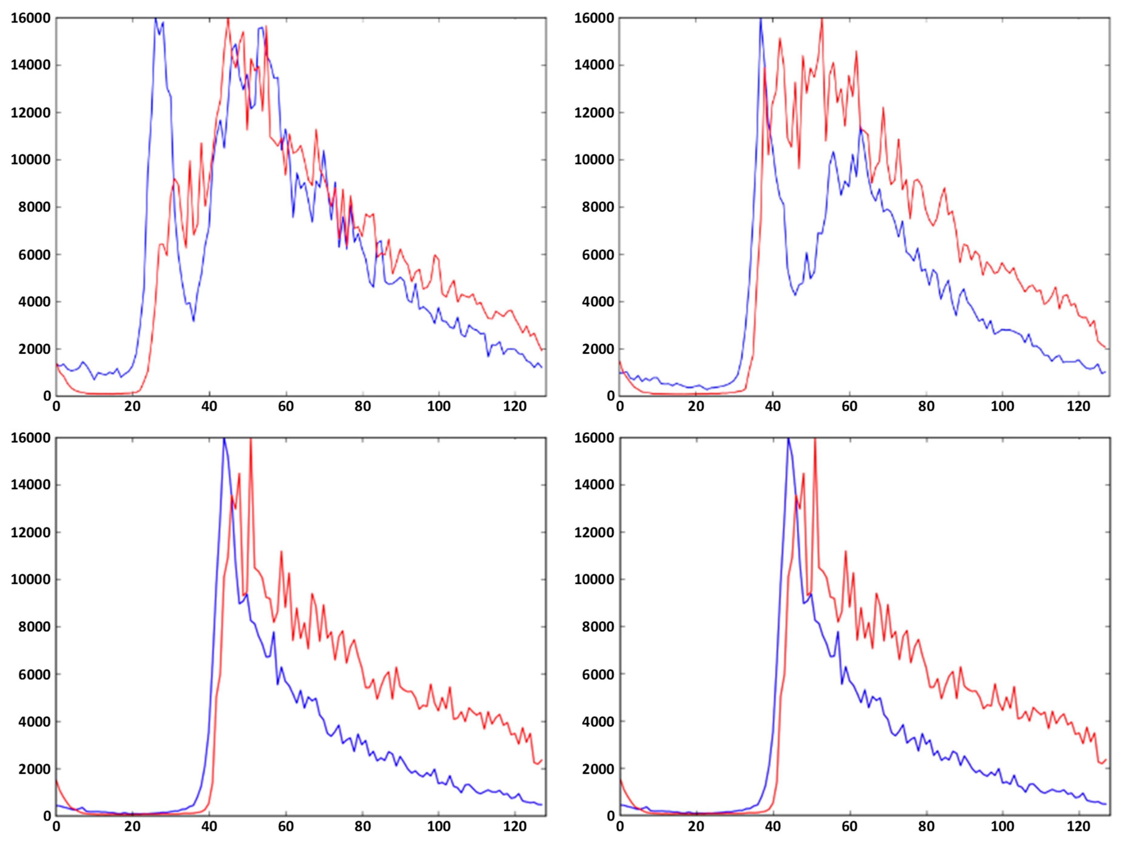
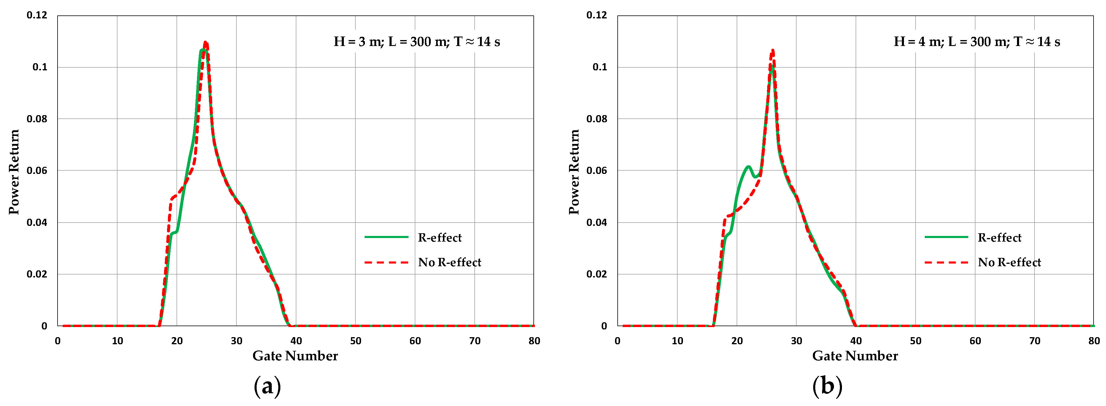
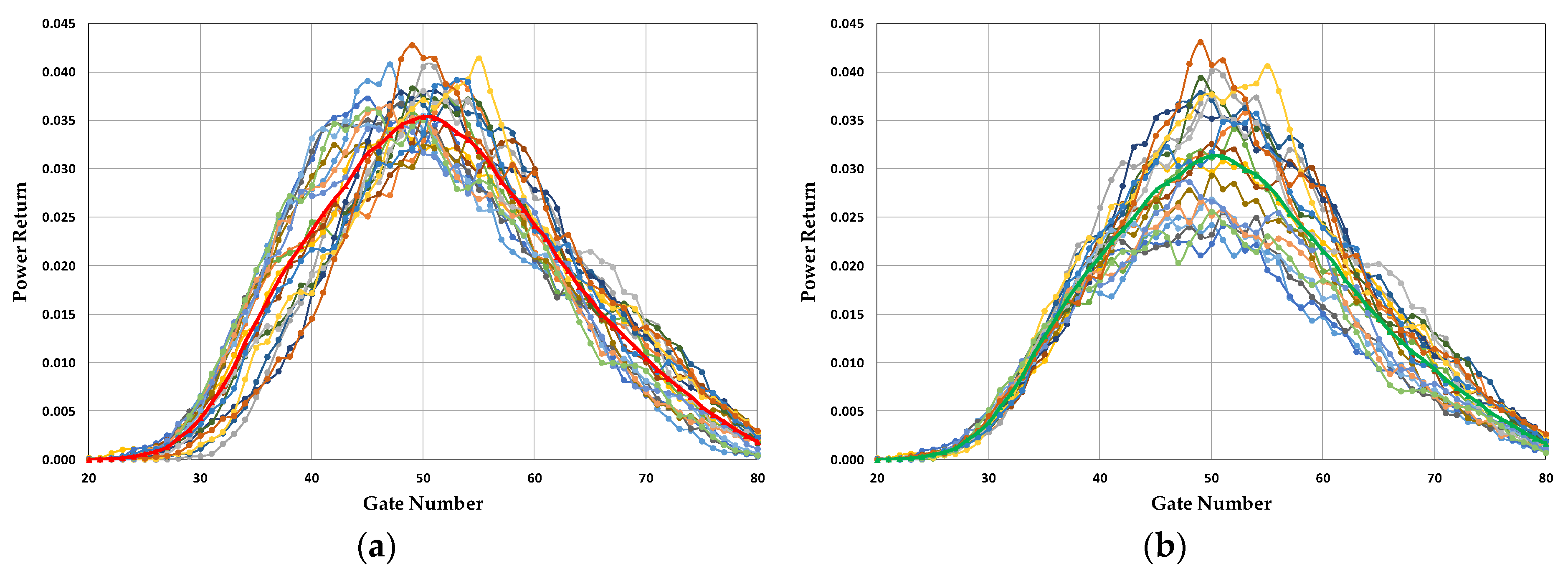
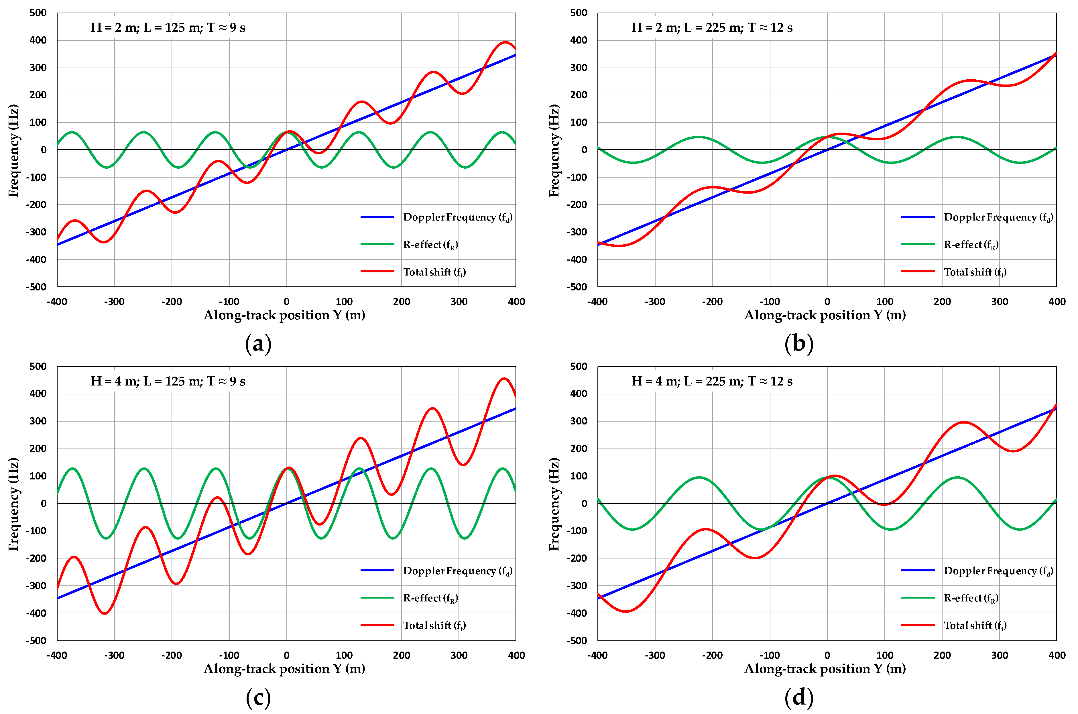
3.1. Single Waveforms

In the following, a few single WF results are reported for monochromatic waves, in order to highlight the basic aspects of the problem. The sea state is assumed to be made up of sine wave-trains in deep water, directed along the flight direction Y. The geometric (size and spatial resolution of the test area) computational parameters are reported in Table 2.
Figure 6 provides a comparison between the waveforms for a single swell wave-train aligned with satellite track (Y direction), computed with, and without, R-effect.
The difference between the two reconstructions is very small, to the point of being negligible: it is most likely that the positive effect (points geometrically outside the nominal Doppler strip moving into the resolution area) is balanced by the negative effect (points exiting the nominal strip).
Things change, sometimes significantly, when the interaction between two wave trains is considered. A common situation is the superimposition of two wave trains, as represented in the following, by adding a wave train of height H1 and a length L1 of a few hundred metres—such as can be expected from a long ocean swell—to a shorter one with height H2 and wavelength L2. Figure 7 shows some results.
The influence of the R-effect is clearly negligible in the case represented in Figure 7a, while it is relevant in the other examples. It is also useful to notice that some of the resulting waveforms bear a similarity to the shapes reported in [11,13] and represented in Figure 1. Similar tests carried out by varying the wavelength and the height of the two components consistently provide a pseudo waveform well different from the classical shape of a Gaussian sea, thus opening new possibilities to use high frequency DDA data to monitor the presence of very long swells, as already suggested in [11,12]. While it appears that the R-effect can, in certain circumstances, affect the formation of DDA response, it is however necessary, in order to get a more realistic appraisal, to take into account what happens when successive measurements are taken from different positions of the satellites, as well as when more realistic sea state is considered.

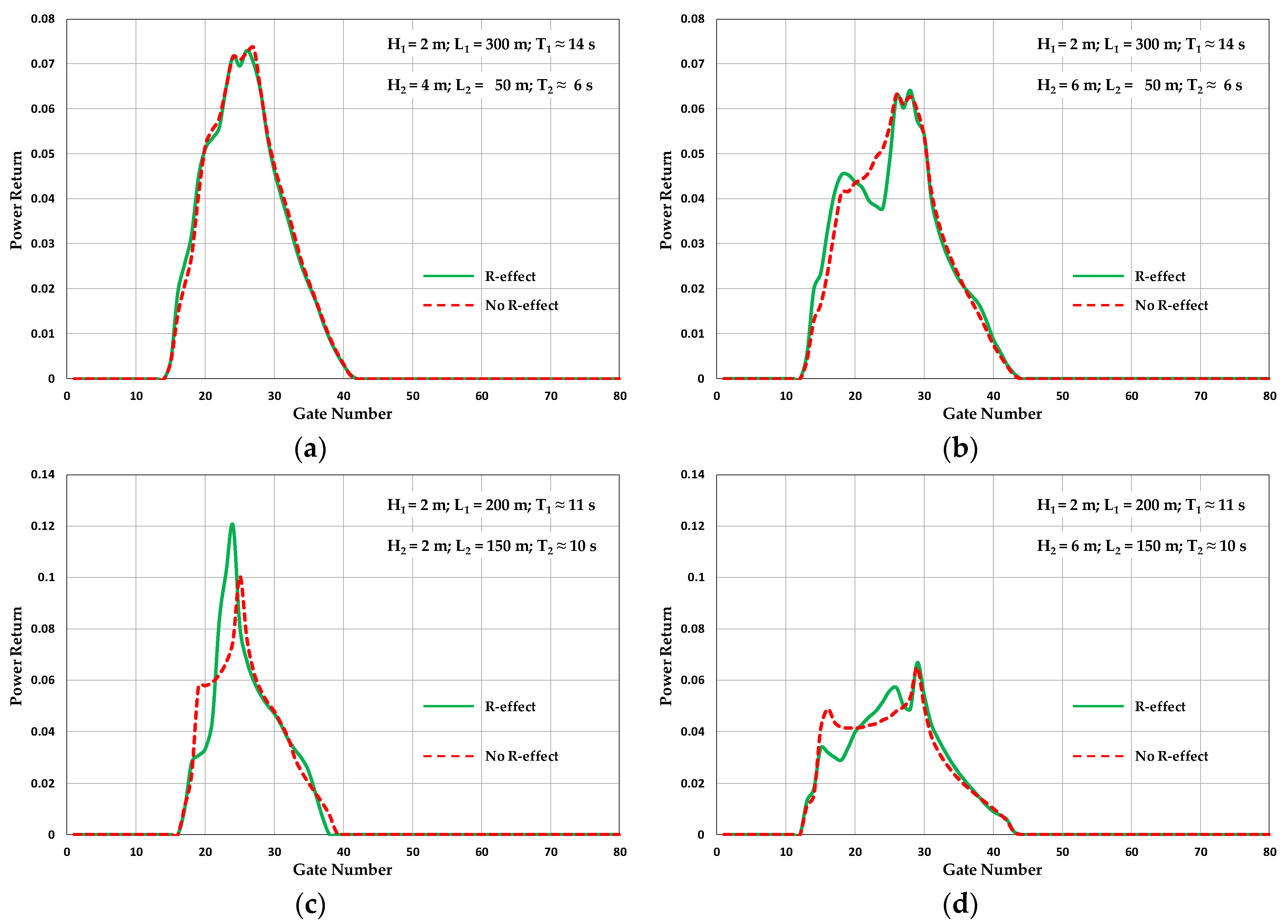
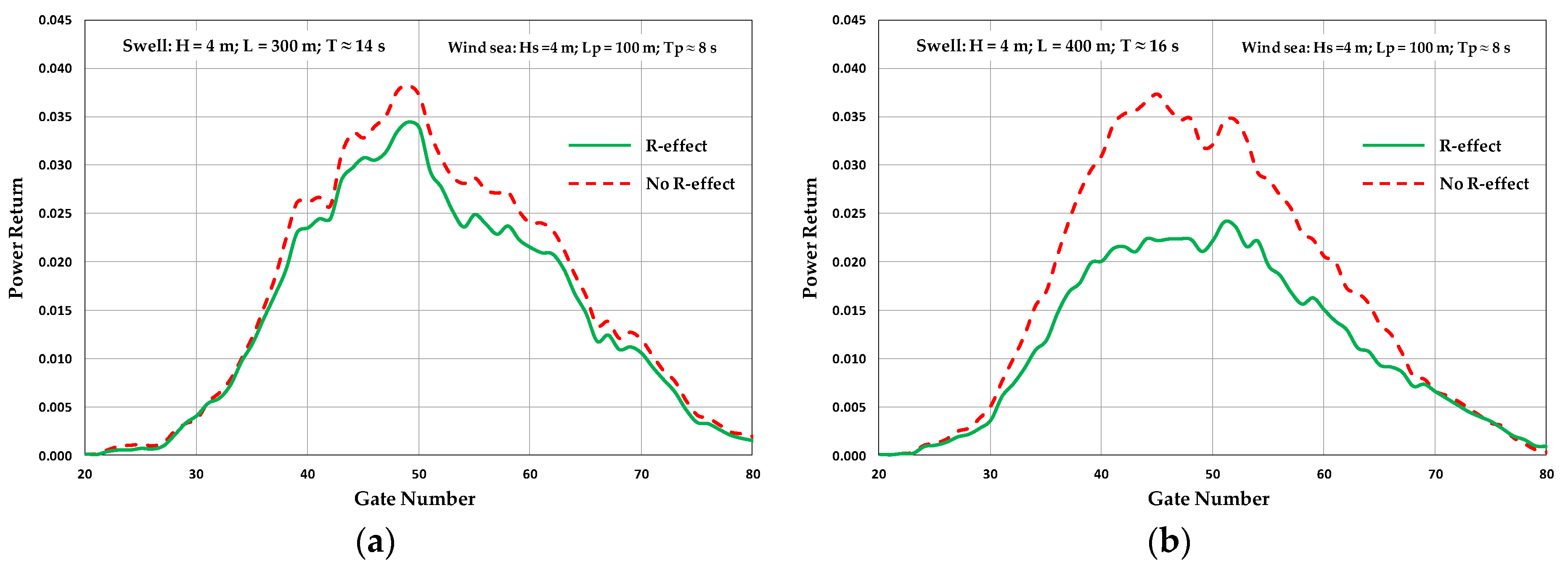
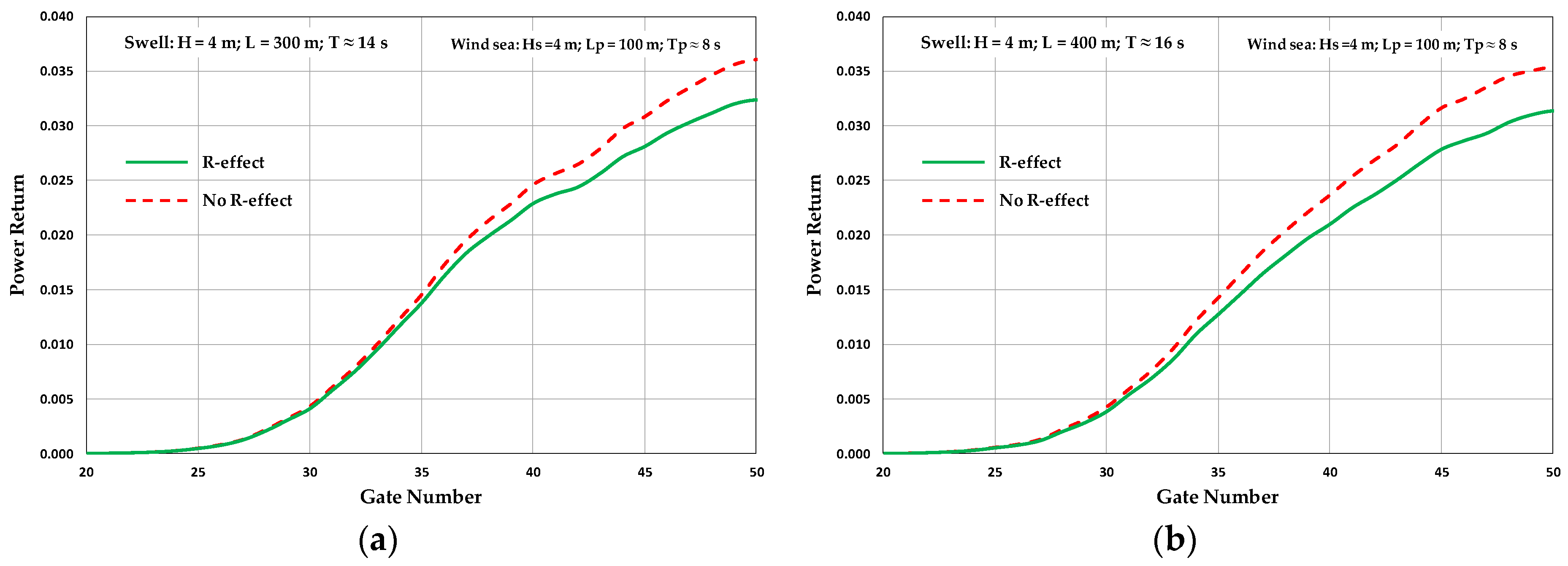
3.2. 20 Hz Data—Wind Sea/Swell Interaction

A common procedure in altimetric sea monitoring is to consider successive measurements at regular intervals, with 20 Hz being the usual standard. Since the satellite velocity is about 7 km/s, a 20 Hz sampling yields a 350 m interval, which is roughly equivalent to the nominal Doppler resolution. A computational algorithm with the following parameters (Table 3) was therefore set up to simulate this procedure.
In order to take into account the interaction between a long swell and a shorter wind sea, a composite sea state was fed into the simulation, based on a JONSWAP spectrum (significant wave height Hs, spreading parameter Sp = 80, and peak wavelength Lp) and a sinusoidal long wave (H, T). Typical results are shown in Figure 8.
The 20 single WFs are reported for both R and non-R-effect simulations. While of course each single waveform is different from the others, it appears that the dispersion of R-effect waveforms is much higher than the dispersion of non-R shapes; also, the comparison of single R and non-R WFs (Figure 9) yields considerable differences.
When average 20 Hz WFs are compared, a consistent difference is evident, the R-WF being less steep (Figure 10) in the leading edge.
The leading edge is actually of particular importance in the extraction algorithms for SWH, such as the ALES (Adaptive Leading Edge Subwaveform) retracker [29,30]. Even if this does not imply an error in the estimation of SWH, since all the algorithms are amply tested and calibrated with experimental data, it could still make sense to verify whether taking the effect into consideration could affect the results.

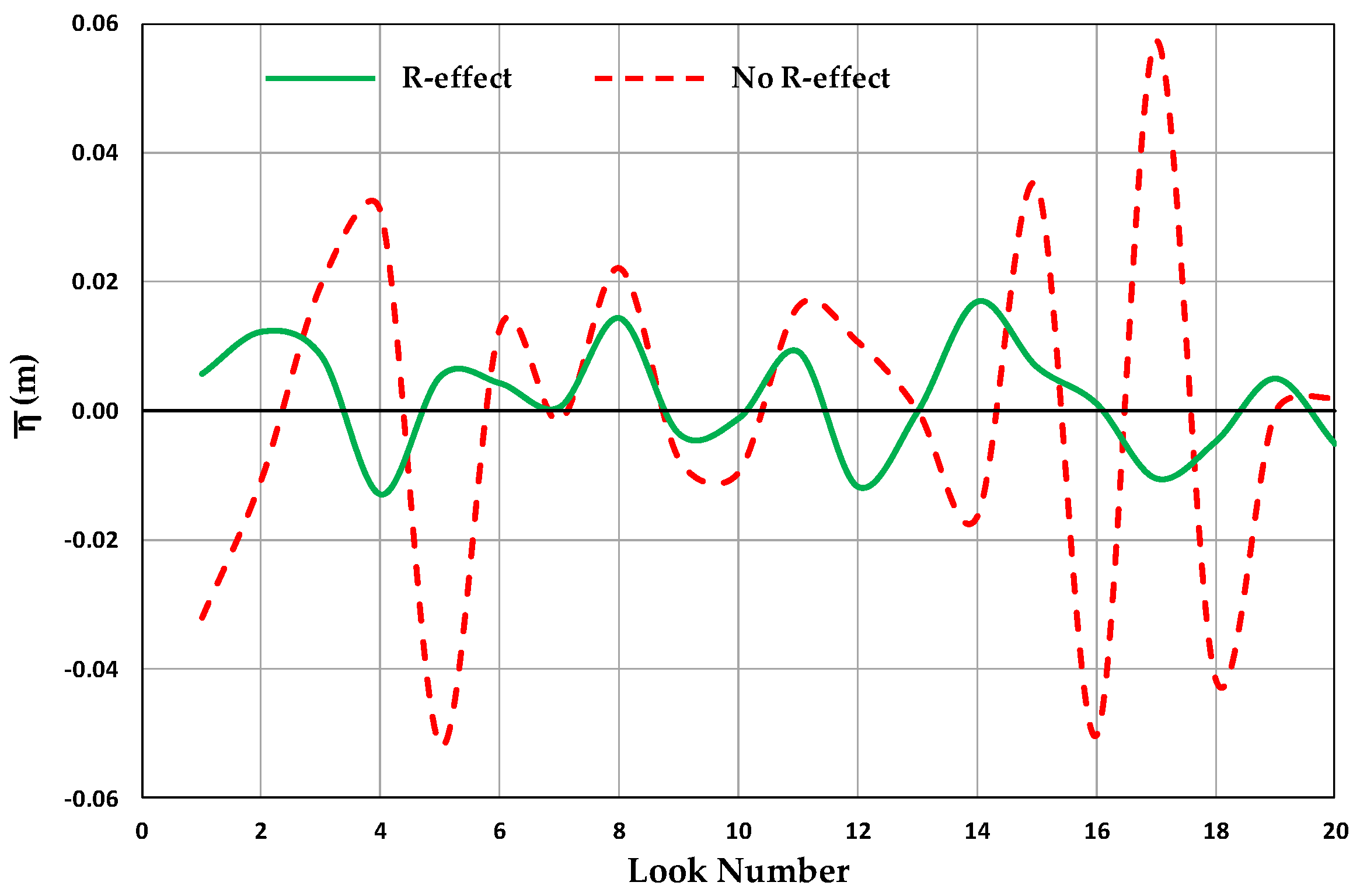
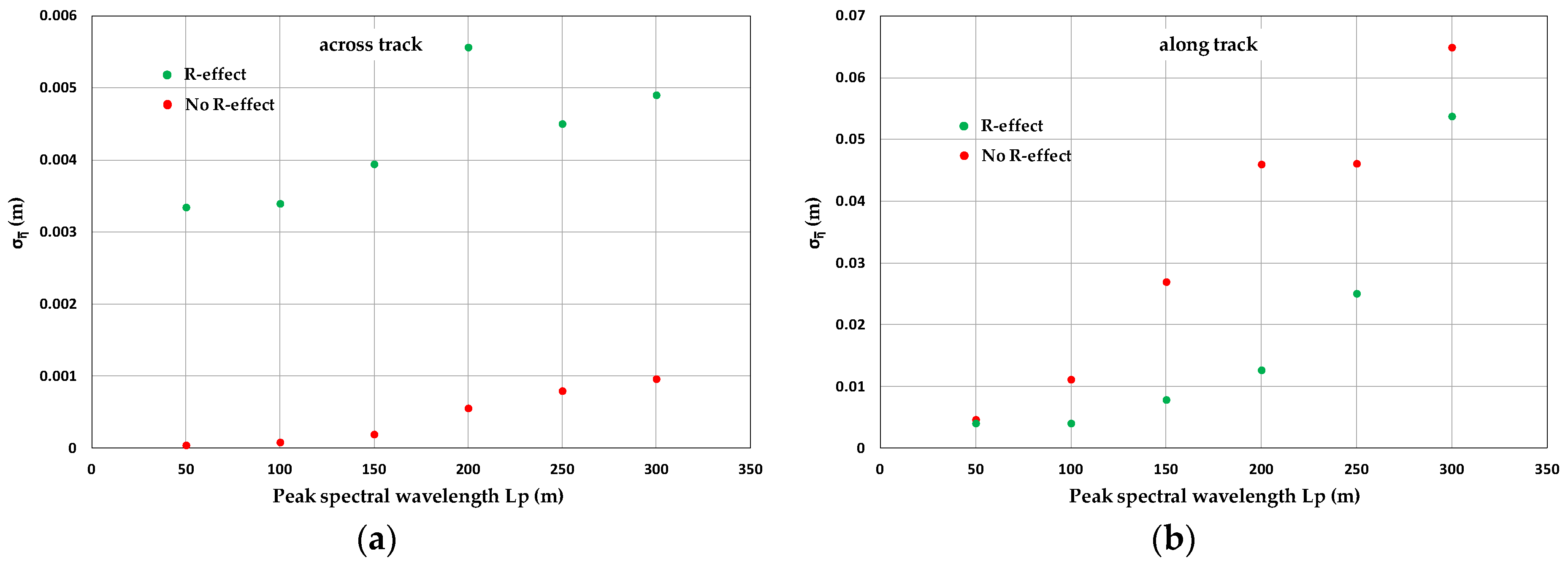
3.3. 20 Hz Data—Sea Surface Height

An important geophysical parameter obtained through satellite altimeter measurement is SSH; in particular, the 20 Hz standard deviation of SSH, also known—perhaps inappropriately—as “SSH error”, is often used as an index to evaluate the quality of this parameter. In order to investigate the possible mechanisms which govern this phenomenon, the simulation has been carried out as above, with a realistic JONSWAP wind sea state, providing 20 results per second. For each of the 20 measurements, the average value η ¯ of the sea surface height over each resolution strip was calculated, both by taking into account, and by neglecting, the R-effect. A typical result is reported in Figure 11.
The SSH errors, i.e., the standard deviations σ η ¯ of the η ¯ over a second (20 looks) can thus be calculated. Figure 12 yields the results for Hs = 4 m and various values of the peak spectral wavelength Lp, both for main wave direction perpendicular (across-track), and aligned (along-track), to the satellite flight direction.
The results are interesting, because they provide an entirely different picture according to whether R effect is taken into account or not. Along-track R results provide—for a 200 m peak wavelength—a σ η ¯ of about 5 mm, while non-R give a negligible value. The reverse is true for across-track results. This leads to the possibility that SSH oscillations, or at least parts of them, might be caused by an aliasing effect. Available experimental information by Fenoglio et al. [8,9], Huang et al. [31], and a simple model by Reale et al. [10] yield very scattered data with an average value of about 1 cm, and a dispersion of the same order of magnitude. Unfortunately, no information is provided in the current literature about the influence of the sea direction with respect to the satellite line of flight, and this is certainly an aspect which should be investigated.

4. Discussion and Conclusions

A number of numerical simulations were performed to evaluate the influence that the R-effect, i.e., the Doppler shift deriving from sea wave orbital movement, can have on the response of delay Doppler altimeters (DDA).
A schematic two-wavelength sea state was first considered; in this condition, the effect is occasionally present and visible in some single waveforms. Another numerical experiment was then carried out, by considering 20 Hz DDA simulated measurements on a more realistic sea state, based on a JONSWAP spectral wind sea superimposed to a long swell. The analysis of the results has shown a minor, but consistent, difference between R and non-R simulations of the 20 Hz averaged waveforms, as well as remarkable differences among some single waveforms; in particular, a complex shape waveform was occasionally found, bearing a similarity with experimental data by other researchers.
A further set of simulations, again based on a JONSWAP wind sea, have provided interesting results on the 20 Hz oscillation σ η ¯ of the SSH. For a sea state orthogonal to the satellite track, the SSH simulated values when the R-effect is considered show a σ η ¯ which could account, at least in part, for the results reported in the literature.
All the results seem to prove that the vertical orbital velocity component does actually influence DDA response; as per the practical importance, however, the conclusions must be more articulate. As per the evaluation of SWH, current algorithms, at least for wind sea states, should not be affected by any error caused by neglecting the R-effect, considering that they have generally been well tested against sea truth. Further detailed investigations should instead be carried on DDA-based monitoring of SWH in the situation where the sea state includes a long swell, and therefore the Gaussian distribution of the water heights does not hold.
Another aspect where the consideration of the R-effect could be meaningful is the analysis of SSH and of its oscillations σ η ¯ : on the one hand, the accuracy requirements of SSH monitoring are higher than those of SWH, on the other hand the behavior of σ η ¯ is a current, active research field. The effect could be exploited to extract further information on the sea state.
A further line of investigation should lead to an assessment of the possible limits of the resolution attainable in the future with satellite DDA.
The consequences of this work might prove to be of relevance, especially taking into account the new generation of sea monitoring satellites, such as Sentinel-3, which are greatly increasing the availability of DDA data over the oceans.

Author Contributions

Conceptualization: F.R. and E.P.C.; methodology: F.R., E.P.C., and F.D.; software: F.R., E.P.C., and A.D.L.; validation: A.D.L. and E.P.C.; formal analysis: E.P.C. and F.R.; writing—original draft preparation: F.R. and E.P.C.; writing—review and editing: A.D.L. and F.D.; supervision: F.D. and F.R. All authors have read and agreed to the published version of the manuscript.

Funding

This research was carried out with University of Salerno Institutional Funds, as well as with the support of CUGRI (University Consortium for Research on Major Hazards).

Acknowledgments

The authors are grateful to T. Moreau and P. Rieu for help and advice, as well as for authorizing the reproduction of the results reported in Figure 1. Thanks are also due to J. Benveniste and P. Cipollini for useful discussion and encouragement over the years, and to the anonymous reviewers for suggesting significant improvements of the approach. Work was partially carried out within ESA EO-Project 1172 “Remote Sensing of Wave Transformation”.

Conflicts of Interest

The authors declare no conflict of interest.

References

  1. Rodriguez, E. Altimetry for non-Gaussian oceans: Height biases and estimation of parameters. J. Geophys. Res. 1988, 93, 14107–14120. [Google Scholar] [CrossRef]
  2. Chelton, D.B.; Ries, J.C.; Haines, B.J.; Fu, L.-L.; Callahan, P.S. Satellite Altimetry. In Satellite Altimetry and Earth Sciences: A Handbook of Techniques and Applications, 1st ed.; Fu, L.-L., Cazenave, A., Eds.; Academic Press: San Diego, CA, USA, 2001; pp. 1–131. [Google Scholar]
  3. Martin-Puig, C.; Ruffini, G.; Marquez, J.; Cotton, P.D.; Srokosz, M.A.; Challenor, P.; Raney, K.; Benveniste, J. Theoretical Model of SAR Altimeter over Water Surfaces. In Proceedings of the IGARSS 2008—2008 IEEE International Geoscience and Remote Sensing Symposium, Boston, MA, USA, 7–11 July 2008; pp. 242–245. [Google Scholar] [CrossRef]
  4. Abdalla, S.; Dinardo, S.; Benveniste, J.; Janssen, P.A.E.M. Assessment of CryoSat-2 SAR mode wind and wave data. Adv. Space Res. 2018, 62, 1421–1433. [Google Scholar] [CrossRef]
  5. Gommenginger, C.P.; Srokosz, M.A. Sea state bias—20 years on. In Proceedings of the Symposium on 15 Years of Progress in Radar Altimetry, Venice, Italy, 13–18 March 2006; Danesy, D., Ed.; ESA-SP 614. ESA Publications Division: Noordwijk, The Netherlands, 2006. [Google Scholar]
  6. Reul, N.; Chapron, B. A model of sea-foam thickness distribution for passive microwave remote sensing applications. J. Geophys. Res. 2003, 108. [Google Scholar] [CrossRef] [Green Version]
  7. Reale, F.; Dentale, F.; Carratelli, E.P. Numerical Simulation of Whitecaps and Foam Effects on Satellite Altimeter Response. Remote Sens. 2014, 6, 3681–3692. [Google Scholar] [CrossRef] [Green Version]
  8. Fenoglio-Marc, L.; Dinardo, S.; Scharro, R.; Lucas, B.; Roland, A.; Dutour Sikiric, M.; Benveniste, J.; Becker, M. Validation of CryoSat-2 in SAR Mode data in the German Bight—Open Ocean. In Proceedings of the OSTST 2014 Meeting “New Frontiers of Altimetry”, Lake Constance, Germany, 28–31 October 2014. [Google Scholar]
  9. Fenoglio-Marc, L.; Dinardo, S.; Scharoo, R.; Roand, A.; Dutour Sikiric, M.; Lucas, B.; Becker, M.; Benveniste, J.; Weiss, R. The German Bight: A validation of CryoSat-2 altimeter data in SAR mode. Adv. Space Res. 2015, 55, 2641–2656. [Google Scholar] [CrossRef]
  10. Reale, F.; Dentale, F.; Pugliese Carratelli, E.; Fenoglio-Marc, L. Influence of Sea State on Sea Surface Height Oscillation from Doppler Altimeter Measurements in the North Sea. Remote Sens. 2018, 10, 1100. [Google Scholar] [CrossRef] [Green Version]
  11. Moreau, T.; Amarouche, L.; Thibaut, P.; Boy, F.; Picot, N. Investigation of swell impact on SAR-mode measurements. In Proceedings of the ESA Living Planet Symposium 2013, Edinburgh, Scotland, 9–13 September 2013. [Google Scholar]
  12. Moreau, T.; Tran, N.; Aublanc, J.; Tison, C.; Le Gac, S.; Boy, F. Impact of long ocean waves on wave height retrieval from SAR altimetry data. Adv. Space Res. 2018, 62, 1434–1444. [Google Scholar] [CrossRef]
  13. Moreau, T.; Labroue, S.; Thibaut, P.; Amarouche, L.; Boy, F.; Picot, N. Sensitivity of SAR mode Altimeter to swells: Attempt to explain sub-mesoscale structures (0.1-1km) seen from SAR. In Proceedings of the CryoSat Third User Workshop, Dresden, Germany, 12–14 March 2013. [Google Scholar]
  14. Reale, F.; Dentale, F.; Fenoglio-Marc, L.; Pugliese Carratelli, E. On the Effect of Wave Vertical Orbital Velocity on Doppler Radar Altimetry. In Proceedings of the 2016 EUMETSAT Meteorological Satellite Conference, Darmstadt, Germany, 26–30 September 2016. [Google Scholar]
  15. Reale, F.; Dentale, F.; Fenoglio-Marc, L.; Pugliese Carratelli, E.; Buchhaupt, C. Wave vertical orbital velocity effects on Doppler Altimeter waveform and SSH measurement. In Proceedings of the 2016 Ocean Surface Topography Science Team (OSTST) Meeting, La Rochelle, France, 1–4 November 2016. [Google Scholar]
  16. Reale, F.; Dentale, F.; Di Leo, A.; Pugliese Carratelli, E. Wave Orbital Velocity Effect on Doppler Radar Altimetry for off-Nadir Beams. In Proceedings of the EUMETSAT Meteorological Satellite Conference 2017, Rome, Italy, 2–6 October 2017. [Google Scholar]
  17. Boisot, O.; Amarouche, L.; Lalaurie, J.-C.; Guérin, C.-A. Dynamical Properties of Sea Surface Microwave Backscatter at Low-Incidence: Correlation Time and Doppler Shift. IEEE Trans. Geosci. Remote Sens. 2016, 54, 7385–7395. [Google Scholar] [CrossRef]
  18. Buchhaupt, C.; Fenoglio, L.; Kusche, J. An Investigation of the Impact of Vertical Water Particle Motions on Fully-Focused SAR Altimetry. In Proceedings of the 2019 Ocean Surface Topography Science Team Meeting, Chicago, IL, USA, 21–25 October 2019. [Google Scholar]
  19. Egido, A.; Ray, R. On the Effect of Surface Motion in SAR Altimeter Observations of the Open Ocean. In Proceedings of the 2019 Ocean Surface Topography Science Team Meeting, Chicago, IL, USA, 21–25 October 2019. [Google Scholar]
  20. Buchhaupt, C. Model Improvement for SAR Altimetry. Ph.D. Thesis, Technischen Universität Darmstadt, Darmstadt, Germany, 27 August 2019. [Google Scholar]
  21. Halimi, A.; Mailhes, C.; Tourneret, J.-Y.; Boy, F.; Picot, N.; Thibaut, P. An analytical model for Doppler altimetry and its estimation algorithm. In Proceedings of the 2012 Ocean Surface Topography Science Team Meeting, Venice, Italy, 22–29 September 2012. [Google Scholar]
  22. Halimi, A.; Mailhes, C.; Tourneret, J.-Y.; Thibaut, P.; Boy, F. A Semi-Analytical Model for Delay/Doppler Altimetry and Its Estimation Algorithm. IEEE Trans. Geosci. Remote Sens. 2014, 52, 4248–4258. [Google Scholar] [CrossRef] [Green Version]
  23. Ray, C.; Martin-Puig, C.; Clarizia, M.P.; Ruffini, G.; Dinardo, S.; Gommenginger, C.; Benveniste, J. SAR Altimeter Backscattered Waveform Model. IEEE Trans. Geosci. Remote Sens. 2015, 53, 911–919. [Google Scholar] [CrossRef]
  24. Boy, F.; Desjonquères, J.; Picot, N.; Moreau, T.; Raynal, M. CryoSat-2 SAR-Mode Over Oceans: Processing Methods, Global Assessment, and Benefits. IEEE Trans. Geosci. Remote Sens. 2017, 55, 148–158. [Google Scholar] [CrossRef]
  25. Hasselmann, K.; Raney, R.K.; Plant, W.J.; Alpers, W.; Shuchman, R.A.; Lyzenga, D.R.; Rufenach, C.L.; Tucker, M.J. Theory of synthetic aperture radar ocean imaging: A MARSEN view. J. Geophys. Res. 1985, 90, 4659–4686. [Google Scholar] [CrossRef]
  26. Pugliese Carratelli, E.; Dentale, F.; Reale, F. Reconstruction of SAR wave image effects through pseudo random simulation. In Proceedings of the Envisat Symposium, Montreux, Switzerland, 23–27 April 2007. European Space Agency, (Special Publication) ESA SP, (SP-636). [Google Scholar]
  27. Benassai, G.; Migliaccio, M.; Montuori, A. Sea wave numerical simulations with COSMO-SkyMed SAR data. J. Coastal Res. 2013, 65, 660–665. [Google Scholar] [CrossRef]
  28. Migliaccio, M.; Montuori, A.; Nunziata, F. X-band Azimuth cut-off for wind speed retrieval by means of COSMO-SkyMed SAR data. In Proceedings of the 2012 IEEE/OES Baltic International Symposium (BALTIC), Klaipeda, Lithuania, 8–10 May 2012. [Google Scholar]
  29. Schlembach, F.; Passaro, M.; Quartly, G.D.; Kurekin, A.; Nencioli, F.; Dodet, G.; Piollé, J.-F.; Ardhuin, F.; Bidlot, J.; Schwatke, C.; et al. Round Robin Assessment of Radar Altimeter Low Resolution Mode and Delay-Doppler Retracking Algorithms for Significant Wave Height. Remote Sens. 2020, 12, 1254. [Google Scholar] [CrossRef] [Green Version]
  30. Passaro, M.; Cipollini, P.; Vignudelli, S.; Quartly, G.D.; Snaith, H.M. ALES: A multi-mission adaptive subwaveform retracker for coastal and open ocean altimetry. Remote Sens. Environ. 2014, 145, 173–189. [Google Scholar] [CrossRef] [Green Version]
  31. Huang, Z.; Wang, H.; Luo, Z.; Shum, C.K.; Tseng, K.-H.; Zhong, B. Improving Jason-2 Sea Surface Heights within 10 km Offshore by Retracking Decontaminated Waveforms. Remote Sens. 2017, 9, 1077. [Google Scholar] [CrossRef]
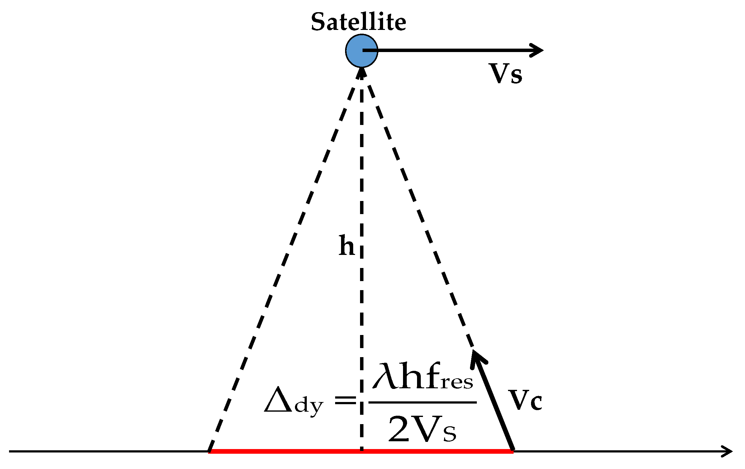
Figure 1. Experimental waveforms both in delay Doppler altimeter (DDA) mode (blue line) and conventional altimeter mode (red line) for various swell events detected by CryoSat-2 altimeter (track 681, cycle 030) as reported in [11].
Jmse 08 00447 g001
Figure 2. Doppler resolution strip along-track (from ESA CryoSat-2 Product Handbook - Baseline D 1.0 - C2-LI-ACS-ESL-5319).
Jmse 08 00447 g002
Figure 3. Along-track resolution as determined by antenna velocity relative to the Earth.
Jmse 08 00447 g003
Figure 4. Effect of particle vertical velocity on the apparent position of an elementary surface area. The red point, positioned in 1, has a positive vertical velocity component VZ1, which adds to its Vc; it therefore appears to be farther (position 1’) from the nadir; the green point, positioned in 2, has a negative VZ2; it therefore looks closer (position 2’).
Jmse 08 00447 g004
Figure 5. Along-track Doppler frequency shift values for different sinusoidal waves: (a) wave height H = 2 m, wavelength L = 125 m, wave period T ≈ 9 s; (b) H = 2 m, L = 225 m, T ≈ 12 s; (c) H = 4 m, L = 125 m, T ≈ 9 s; (d) H = 2, L = 225 m, T ≈ 12 s.
Jmse 08 00447 g005
Figure 6. Simulated waveform with (solid green line), and without (dashed red line), R-effect for two different single sine wave trains: (a) wave height H = 3 m, wavelength L = 300 m, wave period T ≈ 14 s; (b) H = 4 m, L = 300 m, T ≈ 14 s.
Jmse 08 00447 g006
Figure 7. Simulated waveform with (solid green line), and without (dashed red line), R-effect when a longer sinusoidal wave train (wave height H, wavelength L1) is superimposed to a shorter one (wave height H2 and wavelength L2): (a) H2 = 4 m, L2 = 50 m; (b) H2 = 6 m, L2 = 50 m. (c) H2 = 2 m, L2 = 150 m; (d) H2 = 6 m, L2 = 150 m.
Jmse 08 00447 g007
Figure 8. Simulated waveforms on a 20 Hz sample for sinusoidal wave train (wave height H = 4 m, T = 16 s) superimposed to a JONSWAP sea (significant wave height Hs = 4 m; peak period Tp = 8 s): (a) without R-effect (red curve represents the average value); (b) with R-effect (green curve represents the average value).
Jmse 08 00447 g008
Figure 9. Simulated single waveforms with (solid green line), and without (dashed red line), R-effect for swell superimposed to a wind sea: (a) JONSWAP significant wave height Hs = 4 m, peak wave period Tp = 8 s; swell wave height H = 4 m, period T = 14 s; (b) JONSWAP significant wave height Hs = 4 m, peak wave period Tp = 8 s; swell wave height H = 4 m, period T = 16 s.
Jmse 08 00447 g009
Figure 10. Comparison between averaged 20 Hz WF with (green line), and without (dashed red line), R-effect for swell superimposed to a wind sea: (a) JONSWAP significant wave height Hs = 4 m, peak wave period Tp = 8 s; swell wave height H = 4 m, period T = 14 s; (b) JONSWAP significant wave height Hs = 4 m, peak wave period Tp = 8 s; swell wave height H = 4 m, period T = 16 s.
Jmse 08 00447 g010
Figure 11. Sea surface height average values η ¯ by taking in account (solid green line), and by neglecting (dashed red line), the R-effect.
Jmse 08 00447 g011
Figure 12. Standard deviation values σ η ¯ as a function of peak spectral wavelength Lp by considering (green diamonds), and by neglecting (red circles), R-effect: (a) main wave direction across satellite track; (b) main wave direction along satellite track.
Jmse 08 00447 g012
Table 1. Main parameters of CryoSat-2 altimeter in DDA mode.
ParameterValue
Satellite Height h700,000 m
Satellite Velocity VS7000 m/s
Electromagnetic Wavelength λ0.0221 m
Frequency Resolution fres312.5 Hz
Nominal Space Resolution Δdy360.1 m
Table 2. Main parameters of the single measurement numerical simulations
Parameters of the SimulationsValue
Size of test area in across-track (X) direction Lx6000 m
Size of test area in along-track (Y) direction Ly1000 m
Computational grid along the across-track (X) direction DX1 m
Computational grid along the track (Y) direction DY1 m
Resolution of distance between antenna and sea surface0.47 m
Table 3. Main parameters of the multi-look 20 Hz numerical simulations.
Parameters of the SimulationsValue
Size of test area in across-track (X) direction Lx6000 m
Size of test area in along-track (Y) direction Ly6000 m
Computational grid along the across-track (X) direction DX5 m
Computational grid along the track (Y) direction DY5 m
Resolution of distance between antenna and sea surface0.35 m
Number of measurements in a second20 Hz

