Lidar Observations of the Swash Zone of a Low-Tide Terraced Tropical Beach under Variable Wave Conditions: The Nha Trang (Vietnam) COASTVAR Experiment

 , ,
, ,  ,
,  , , and
Abstract
Highlights
- Nine-day detailed swash hydro-morphodynamic measurements of wave induced erosion and recovery on a tropical beach (Nha Trang, Vietnam) with a Lidar.
- The wave height measured on the lower foreshore and active slope are key parameters to predict vertical run-up on this type of intermediate beach.
- Tide induces a strong modulation of wave action and drives large intra- and daily changes on the swash zone.
1. Introduction
2. Methods
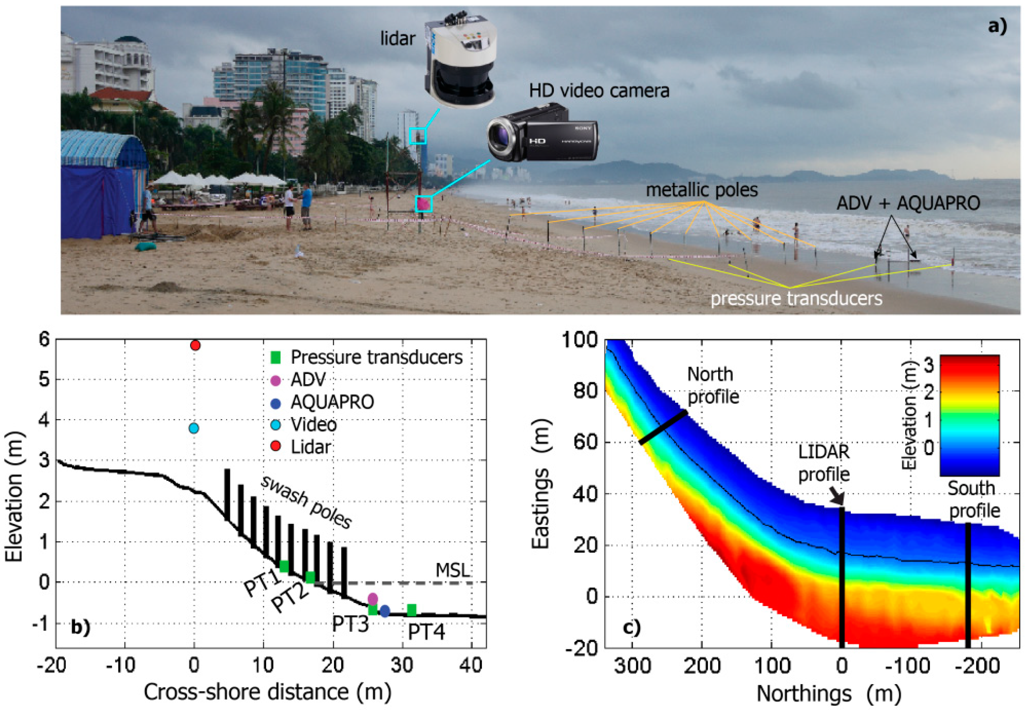
2.1. Study Area
2.2. Experimental Set-up
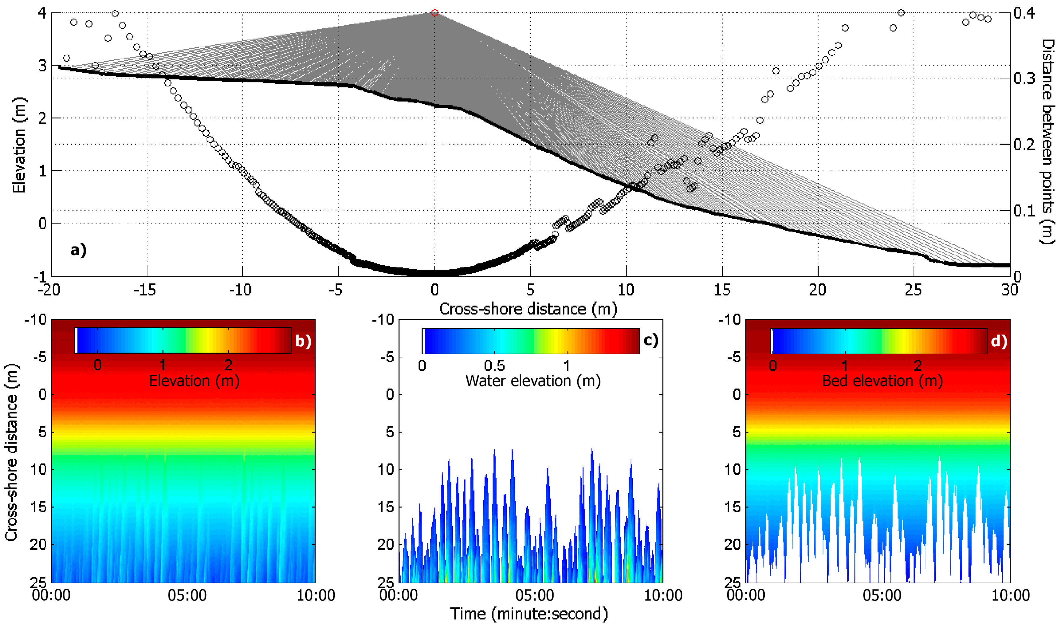
2.3. Two-Dimensional Lidar
3. Results
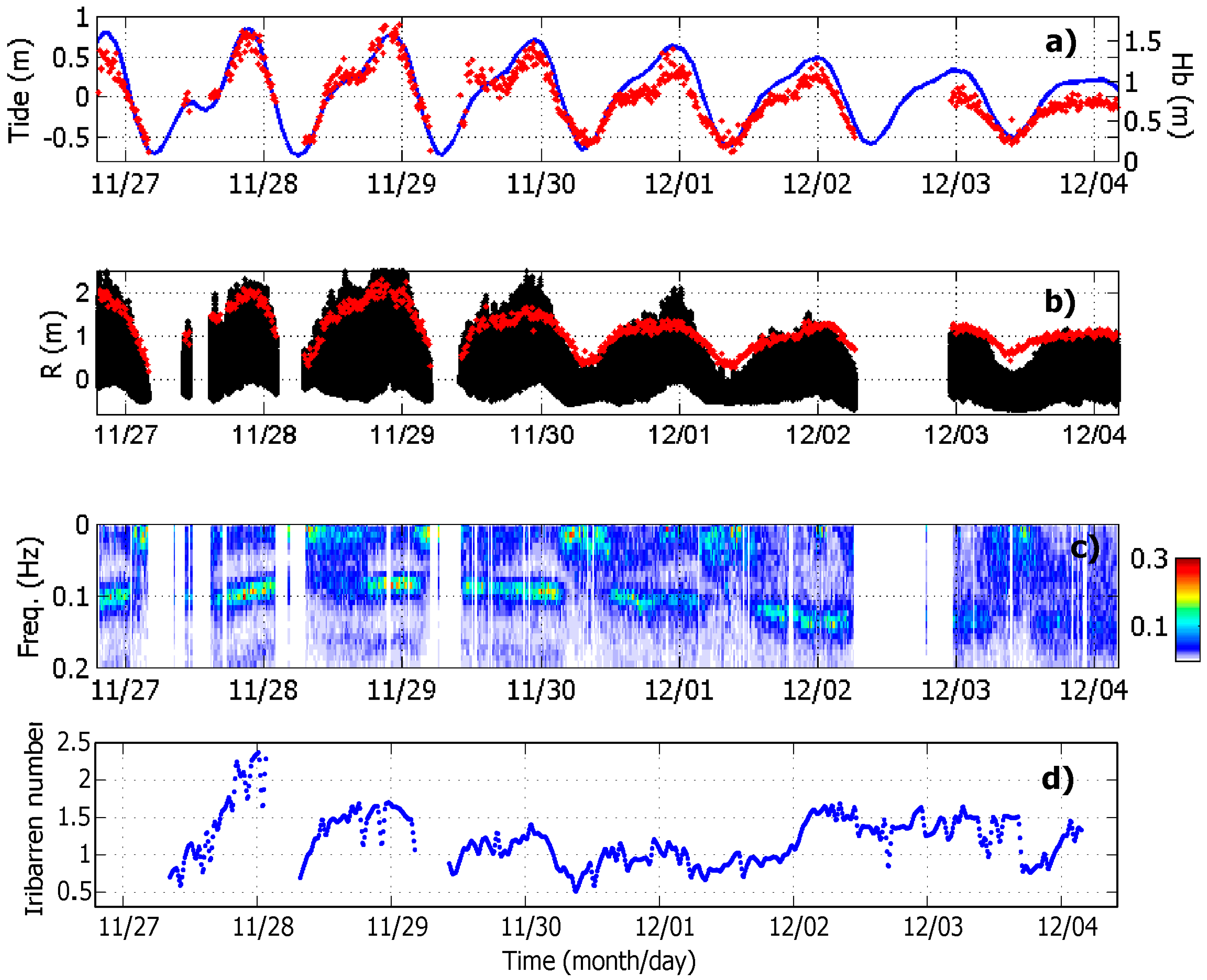
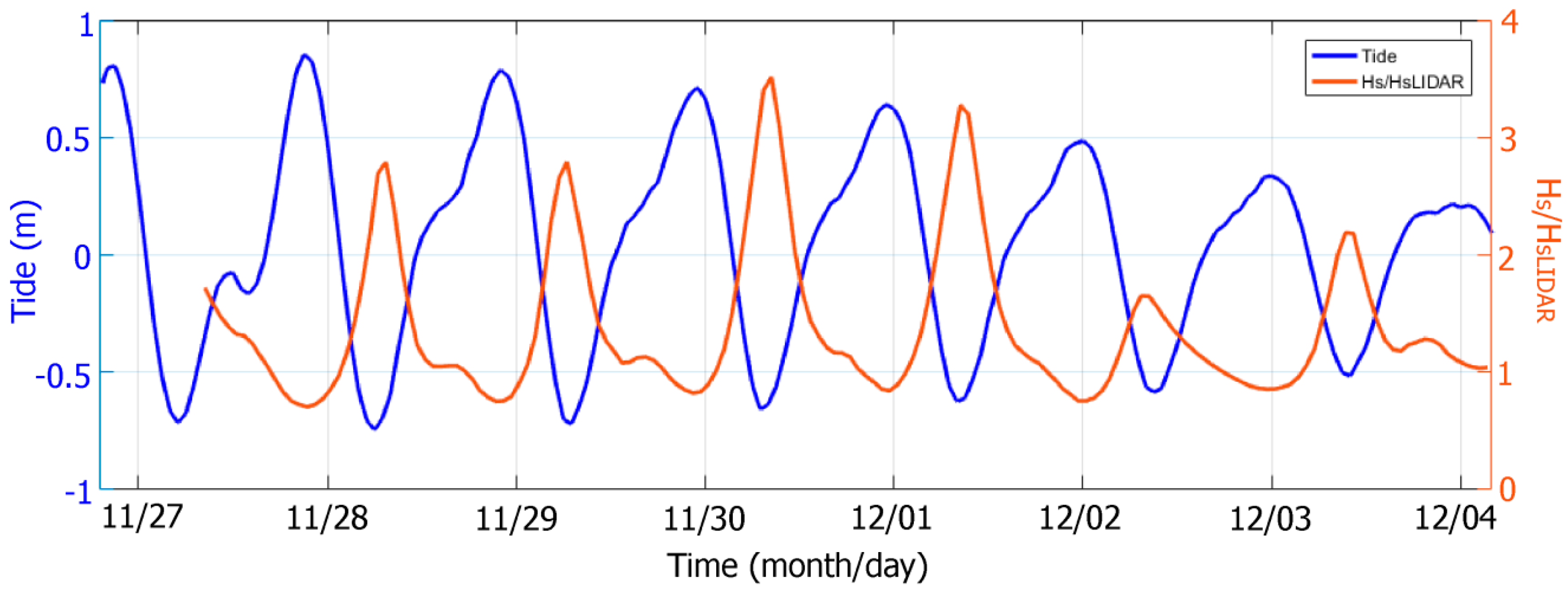
3.1. Offshore Wave Forcing
3.2. Wave Characteristics and Run-up Observed from the Lidar
3.3. Daily Morphological Evolution
3.4. Intra-Tidal Morphological Evolution
3.5. Morphological Evolution and Hydrodynamic Forcing
4. Discussion
4.1. Tidal Modulation of Waves and Run-Up Heights
4.2. Upper-Beach Erosion and Recovery
4.2.1. Daily Evolution
4.2.2. Intra-Tidal Profile Evolution
5. Conclusions
Author Contributions
Funding
Acknowledgments
Conflicts of Interest
References
- Schepper, R.; De Vries, S.; Reniers, A.; Katsman, C.; Almar, R.; Bergsma, E.; Davidson, M. Multi-timescale shoreline modelling. Coast. Sediments 2019, 2200–2210. [Google Scholar] [CrossRef]
- Raubenheimer, B.; Guza, R. Observations and predictions of run-up. J. Geophys. Res. Ocean. 1996, 101, 25575–25587. [Google Scholar] [CrossRef]
- Ruggiero, P.; Holman, R.A.; Beach, R. Wave run-up on a high-energy dissipative beach. J. Geophys. Res. Ocean. 2004, 109. [Google Scholar] [CrossRef]
- Wright, L.; Short, A.D. Morphodynamic variability of surf zones and beaches: A synthesis. Mar. Geol. 1984, 56, 93–118. [Google Scholar] [CrossRef]
- Miles, J.; Russell, P. Dynamics of a reflective beach with a low tide terrace. Cont. Shelf Res. 2004, 24, 1219–1247. [Google Scholar] [CrossRef]
- Almar, R.; Almeida, P.; Blenkinsopp, C.; Catalán, P. Surf-swash interactions on a low-tide terraced beach. J. Coast. Res. 2016, 75, 348–352. [Google Scholar] [CrossRef]
- Aagaard, T.; Greenwood, B.; Hughes, M. Sediment transport on dissipative, intermediate and reflective beaches. Earth Sci. Rev. 2013, 124, 32–50. [Google Scholar] [CrossRef]
- Aagaard, T.; Hughes, M.G. Breaker turbulence and sediment suspension in the surf zone. Mar. Geol. 2010, 271, 250–259. [Google Scholar] [CrossRef]
- Puleo, J.; Beach, R.; Holman, R.A.; Allen, J. Swash zone sediment suspension and transport and the importance of bore-generated turbulence. J. Geophys. Res. Ocean. 2000, 105, 17021–17044. [Google Scholar] [CrossRef]
- Petti, M.; Longo, S. Turbulence experiments in the swash zone. Coast. Eng. 2001, 43, 1–24. [Google Scholar] [CrossRef]
- Shen, M.; Meyer, R. Climb of a bore on a beach Part 3. Run-up. J. Fluid Mech. 1963, 16, 113–125. [Google Scholar] [CrossRef]
- Hughes, M.G.; Moseley, A.S. Hydrokinematic regions within the swash zone. Cont. Shelf Res. 2007, 27, 2000–2013. [Google Scholar] [CrossRef]
- Power, H.; Holman, R.; Baldock, T. Swash zone boundary conditions derived from optical remote sensing of swash zone flow patterns. J. Geophys. Res. Ocean. 2011, 116. [Google Scholar] [CrossRef]
- Almar, R.; Blenkinsopp, C.; Almeida, L.; Cienfuegos, R.; Catalán, P. A new remote predictor of wave reflection based on run-up asymmetry. Estuar. Coast. Shelf Sci. 2018, 217, 1–8. [Google Scholar] [CrossRef]
- Masselink, G.; Puleo, J.A. Swash-zone morphodynamics. Cont. Shelf Res. 2006, 26, 661–680. [Google Scholar] [CrossRef]
- Hardisty, J.; Collier, J.; Hamilton, D. A calibration of the Bagnold beach equation. Mar. Geol. 1984, 61, 95–101. [Google Scholar] [CrossRef]
- Kulkarni, C.D.; Levoy, F.; Monfort, O.; Miles, J. Morphological variations of a mixed sediment beachface (Teignmouth, UK). Cont. Shelf Res. 2004, 24, 1203–1218. [Google Scholar] [CrossRef]
- Strahler, A.N. Tidal cycle of changes in an equilibrium beach, Sandy Hook, New Jersey. J. Geol. 1966, 74, 247–268. [Google Scholar] [CrossRef]
- Austin, M.J.; Buscombe, D. Morphological change and sediment dynamics of the beach step on a macrotidal gravel beach. Mar. Geol. 2008, 249, 167–183. [Google Scholar] [CrossRef]
- Masselink, G.; Li, L. The role of swash infiltration in determining the beachface gradient: A numerical study. Mar. Geol. 2001, 176, 139–156. [Google Scholar] [CrossRef]
- Turner, I.L.; Russell, P.E.; Butt, T. Measurement of wave-by-wave bed-levels in the swash zone. Coast. Eng. 2008, 55, 1237–1242. [Google Scholar] [CrossRef]
- Ibaceta, R.; Almar, R.; Lefebvre, J.P.; Mensah-Senoo, T.; Layrea, W.S. High frequency monitoring of swash hydro-morphodynamics on a reflective beach (Grand Popo, Benin): A new method. In Proceedings of the 34th Conference on Coastal Engineering, Seoul, Korea, 15–20 June 2014. [Google Scholar]
- Ibaceta, R.; Almar, R.; Catalán, P.A.; Blenkinsopp, C.E.; Almeida, L.P.; Cienfuegos, R. Assessing the Performance of a Low-Cost Method for Video-Monitoring the Water Surface and Bed Level in the Swash Zone of Natural Beaches. Remote Sens. 2018, 10, 49. [Google Scholar] [CrossRef]
- Brodie, K.L.; Raubenheimer, B.; Elgar, S.; Slocum, R.K.; McNinch, J.E. Lidar and pressure measurements of inner-surfzone waves and setup. J. Atmos. Ocean. Technol. 2015, 32, 1945–1959. [Google Scholar] [CrossRef]
- Martins, K.; Blenkinsopp, C.E.; Zang, J. Monitoring individual wave characteristics in the inner surf with a 2-dimensional laser scanner (Lidar). J. Sens. 2016, 2016, 7965431. [Google Scholar] [CrossRef]
- Martins, K.; Blenkinsopp, C.E.; Power, H.E.; Bruder, B.; Puleo, J.A.; Bergsma, E.W.J. High-resolution monitoring of wave transformation in the surf zone using a Lidar scanner array. Coast. Eng. 2017, 128, 37–43. [Google Scholar] [CrossRef]
- Blenkinsopp, C.; Mole, M.; Turner, I.; Peirson, W. Measurements of the time-varying free-surface profile across the swash zone obtained using an industrial LIDAR. Coast. Eng. 2010, 57, 1059–1065. [Google Scholar] [CrossRef]
- Vousdoukas, M.; Kirupakaramoorthy, T.; Oumeraci, H.; De La Torre, M.; Wübbold, F.; Wagner, B.; Schimmels, S. The role of combined laser scanning and video techniques in monitoring wave-by-wave swash zone processes. Coast. Eng. 2014, 83, 150–165. [Google Scholar] [CrossRef]
- Almeida, L.; Masselink, G.; Russell, P.; Davidson, M. Observations of gravel beach dynamics during high energy wave conditions using a laser scanner. Geomorphology 2015, 228, 15–27. [Google Scholar] [CrossRef]
- Martins, K.; Blenkinsopp, C.E.; Deigaard, R.; Power, H.E. Energy Dissipation in the Inner Surf Zone: New Insights from Lidar-Based Roller Geometry Measurements. J. Geophys. Res. Ocean. 2018, 123, 3386–3407. [Google Scholar] [CrossRef]
- Bergsma, E.W.J.; Blenkinsopp, C.E.; Martins, K.; Almar, R.; de Almeida, L.P.M. Bore collapse and wave run-up on a sandy beach. Cont. Shelf Res. 2019, 174, 132–139. [Google Scholar] [CrossRef]
- O’Dea, A.; Brodie, K.L.; Hartzell, P. Continuous Coastal Monitoring with an Automated Terrestrial Lidar Scanner. J. Mar. Sci. Eng. 2019, 7, 37. [Google Scholar] [CrossRef]
- Almar, R.; Blenkinsopp, C.; Almeida, L.P.; Bergsma, E.W.; Catalan, P.A.; Cienfuegos, R.; Viet, N.T. Complex intertidal beach profile estimation from reflected wave measurements. Coast. Eng. 2019, 151, 58–63. [Google Scholar] [CrossRef]
- Almar, R.; Marchesiello, P.; Almeida, L.P.; Thuan, D.H.; Tanaka, H.; Viet, N.T. Shoreline Response to a Sequence of Typhoon and Monsoon Events. Water 2017, 9, 364. [Google Scholar] [CrossRef]
- Lefebvre, J.P.; Almar, R.; Viet, N.T.; Thuan, D.H.; Binh, L.T.; Ibaceta, R.; Duc, N.V. Contribution of swash processes generated by low energy wind waves in the recovery of a beach impacted by extreme events: Nha Trang, Vietnam. J. Coast. Res. 2014, 70, 663–668. [Google Scholar] [CrossRef]
- Mau, L.D. Overview of Natural Geographical Conditions of Nha Trang Bay; Technical Report; Nha Trang Institute of Oceanography: Nha Trang, Vietnam, 2014. [Google Scholar]
- Almeida, L.; Almar, R.; Meyssignac, B.; Viet, N. Contributions to Coastal Flooding Events in Southeast of Vietnam and their link with Global Mean Sea Level Rise. Geosciences 2018, 8, 437. [Google Scholar] [CrossRef]
- Thuan, D.H.; Binh, L.T.; Viet, N.T.; Hanh, D.K.; Almar, R.; Marchesiello, P. Typhoon impact and recovery from continuous video monitoring: A case study from Nha Trang Beach, Vietnam. J. Coast. Res. 2016, 75, 263–267. [Google Scholar] [CrossRef]
- Hanh, P.T.T.; Furukawa, M. Impact of sea level rise on coastal zone of Vietnam. Bull. Coll. Sci. Univ. 2007, 84, 45. [Google Scholar]
- Andriolo, U.; Almeida, L.P.; Almar, R. Coupling terrestrial Lidar and video imagery to perform 3D intertidal beach topography. Coast. Eng. 2018, 140, 232–239. [Google Scholar] [CrossRef]
- Battjes, J.A. Surf similarity. In Proceedings of the 14th International Conference on Coastal Engineering, Copenhagen, Denmark, 24–28 June 1974. [Google Scholar]
- Brodie, K.L.; Slocum, R.K.; McNinch, J.E. New insights into the physical drivers of wave run-up from a continuously operating terrestrial laser scanner. In Proceedings of the 2012 Oceans—IEEE, Hampton Roads, VA, USA, 14–19 October 2012. [Google Scholar]
- Waddell, E. Dynamics of Swash and Implication to Beach Response; Technical Report; Louisiana State University, Coastal Studies Institute: Baton Rouge, LA, USA, 1973. [Google Scholar]
- Stockdon, H.F.; Holman, R.A.; Howd, P.A.; Sallenger, A.H. Empirical parameterization of setup, swash, and run-up. Coast. Eng. 2006, 53, 573–588. [Google Scholar] [CrossRef]
- Hunt, I.A. Design of sea walls and bkeakwaters. J. Waterw. Ports Ocean Eng. 1959, 85, 123–152. [Google Scholar]
- Holman, R.A. Extreme value statistics for wave run-up on a natural beach. Coast. Eng. 1986, 9, 527–544. [Google Scholar] [CrossRef]
- Gomes da Silva, P.; Medina, R.; González, M.; Garnier, R. Wave reflection and saturation on natural beaches: The role of the morphodynamic beach state in incident swash. Coast. Eng. 2019, 153, 103540. [Google Scholar] [CrossRef]
- Guedes, R.M.C.; Bryan, K.R.; Coco, G.; Holman, R. The effects of tides on swash statistics on an intermediate beach. J. Geophys. Res. Ocean. 2011, 116. [Google Scholar] [CrossRef]
- Gomes da Silva, P.; Coco, G.; Garnier, R.; Klein, A.H.F. On the prediction of run-up, setup and swash on beaches. Earth Sci. Rev. 2020, 204, 103148. [Google Scholar] [CrossRef]
- Khoury, A.; Jarno, A.; Marin, F. Experimental study of run-up for sandy beaches under waves and tide. Coast. Eng. 2019, 144, 33–46. [Google Scholar] [CrossRef]
- Blenkinsopp, C.E.; Matias, A.; Howe, D.; Castelle, B.; Marieu, V.; Turner, I.L. Wave runup and overwash on a prototype-scale sand barrier. Coast. Eng. 2016, 113, 88–103. [Google Scholar] [CrossRef]
- Hine, A.C. Mechanisms of berm development and resulting beach growth along a barrier spit complex. Sedimentology 1979, 26, 333–351. [Google Scholar] [CrossRef]
- Weir, F.M.; Hughes, M.G.; Baldock, T.E. Beach face and berm morphodynamics fronting a coastal lagoon. Geomorphology 2006, 82, 331–346. [Google Scholar] [CrossRef]
- Poate, T.; Masselink, G.; Davidson, M.; McCall, R.; Russell, P.; Turner, I. High frequency in-situ field measurements of morphological response on a fine gravel beach during energetic wave conditions. Mar. Geol. 2013, 342, 1–13. [Google Scholar] [CrossRef]
- Grant, U.S. Influence of the water table on beach aggradation and degradation. J. Mar. Res. 1948, 7, 655–660. [Google Scholar]
- Duncan, J.R. The effects of water table and tide cycle on swash-backwash sediment distribution and beach profile development. Mar. Geol. 1964, 2, 186–197. [Google Scholar] [CrossRef]
- Brocchini, M.; Baldock, T. Recent advances in modeling swash zone dynamics: Influence of surf-swash interaction on nearshore hydrodynamics and morphodynamics. Rev. Geophys. 2008, 46. [Google Scholar] [CrossRef]


| Parameter | High-Tide | Mid-Tide | Low-Tide | |||
|---|---|---|---|---|---|---|
| r2 | RMSE (m) | r2 | RMSE (m) | r2 | RMSE (m) | |
| (HsLo)0.5 | 0.68 | 1.01 | 0.35 | 1.3 | 0.3 | 1.5 |
| tanβ(HsLo)0.5 | 0.85 | 0.2 | 0.64 | 0.19 | 0.65 | 0.13 |
| tanβ(HsLIDARLo)0.5 | 0.88 | 0.2 | 0.77 | 0.16 | 0.83 | 0.07 |
© 2020 by the authors. Licensee MDPI, Basel, Switzerland. This article is an open access article distributed under the terms and conditions of the Creative Commons Attribution (CC BY) license (http://creativecommons.org/licenses/by/4.0/).
Share and Cite
Almeida, L.P.; Almar, R.; Blenkinsopp, C.; Senechal, N.; Bergsma, E.; Floc’h, F.; Caulet, C.; Biausque, M.; Marchesiello, P.; Grandjean, P.; et al. Lidar Observations of the Swash Zone of a Low-Tide Terraced Tropical Beach under Variable Wave Conditions: The Nha Trang (Vietnam) COASTVAR Experiment. J. Mar. Sci. Eng. 2020, 8, 302. https://doi.org/10.3390/jmse8050302
Almeida LP, Almar R, Blenkinsopp C, Senechal N, Bergsma E, Floc’h F, Caulet C, Biausque M, Marchesiello P, Grandjean P, et al. Lidar Observations of the Swash Zone of a Low-Tide Terraced Tropical Beach under Variable Wave Conditions: The Nha Trang (Vietnam) COASTVAR Experiment. Journal of Marine Science and Engineering. 2020; 8(5):302. https://doi.org/10.3390/jmse8050302
Chicago/Turabian StyleAlmeida, Luís Pedro, Rafael Almar, Chris Blenkinsopp, Nadia Senechal, Erwin Bergsma, France Floc’h, Charles Caulet, Melanie Biausque, Patrick Marchesiello, Philippe Grandjean, and et al. 2020. "Lidar Observations of the Swash Zone of a Low-Tide Terraced Tropical Beach under Variable Wave Conditions: The Nha Trang (Vietnam) COASTVAR Experiment" Journal of Marine Science and Engineering 8, no. 5: 302. https://doi.org/10.3390/jmse8050302
APA StyleAlmeida, L. P., Almar, R., Blenkinsopp, C., Senechal, N., Bergsma, E., Floc’h, F., Caulet, C., Biausque, M., Marchesiello, P., Grandjean, P., Ammann, J., Benshila, R., Thuan, D. H., Gomes da Silva, P., & Viet, N. T. (2020). Lidar Observations of the Swash Zone of a Low-Tide Terraced Tropical Beach under Variable Wave Conditions: The Nha Trang (Vietnam) COASTVAR Experiment. Journal of Marine Science and Engineering, 8(5), 302. https://doi.org/10.3390/jmse8050302