Shoaling Waves Interacting with an Orthogonal Current

Abstract

In the present work, an experimental investigation on the hydrodynamics of shoaling waves superposed on a steady orthogonal current is carried out. An experimental campaign in a wave tank has been performed, with waves and current interacting at a right angle over a sloping planar beach. Velocity data have been gathered during the experiments in order to investigate mean, phase and turbulent flow. A detailed preliminary analysis of the time- and space-variability of the experiments is presented. Results show that a complex interaction between waves and current occurs as the wave shoals, in terms of sheer production, momentum transfer and turbulent mixing. Superposition of waves determines a shear increase at the bottom due to an enhanced turbulence mixing, nonetheless as depth decreases and the current velocity consequently increases, shoaling waves may be less efficient in enhancing shear at the bottom. Moreover, the superposition of waves determines the current to oscillate around its mean velocity value. Nevertheless, as wave shoals and simultaneously current velocity increases with decreasing depth, waves and current oscillatory motion experience a phase lag, as a response of the larger momentum of the current to the changing of the shoaling waves acceleration distribution along the wave phase. Moreover, the turbulent bursting events of the combined flow in proximity of the bed have been investigated by means of quadrant analysis, showing an increase of the turbulent ejections and sweeps due to the superposition of the shoaling waves.

1. Introduction

Waves and currents are generally simultaneously present in coastal environments. It is widely known that the superposition of waves significantly alters the mean current flow hydrodynamics, moreover, their combined flow drives important coastal processes such as sediment transport. Wave-current interaction (WCI) has been experimentally investigated considering waves following and opposing the current direction [1,2,3], in the presence of nonlinear waves [4,5] in the presence of rough beds or fixed bedforms [6,7].

Progress has also been made in the development of theoretical [8,9,10,11,12,13] and numerical models [14,15,16] of WCI. Most of the existing models have been validated through laboratory experiments on collinear waves and currents, despite WCI in the nearshore usually occurs with a near-orthogonal angle. Indeed, due to difficulties in the physical modeling, experimental data on wave-current interaction at a right angle are relatively scarce. Moreover, although WCI generally occurs on sloping sandy beaches, to the authors knowledge, the existing studies have considered horizontal bottom, with very few exceptions [17]. Musumeci et al. [18] investigated orthogonal WCI over sand and gravel bottoms in a 3D tank, showing that the apparent bottom roughness may be increased due to waves, depending on the turbulent regime in the wave bottom boundary layer. Moreover, an oscillatory flow out of phase with respect to the wave velocity has been observed in the current direction in the presence of combined flows. Faraci et al. [19] investigated combined waves and currents over fixed ripples through numerical and laboratory tests. Results showed that the presence of ripples acts as a macroroughness, inducing turbulence to intensify and current apparent roughness to increase. Fernando et al. [13] carried out experiments on WCI at a right angle in a wave basin over a movable horizontal bed and compared results with theoretical nonlinear models of wave-current combined flow. Results showed that for the larger wave heights none of the models was able to properly reconstruct the observed velocity profile, whereas for smaller wave heights most of the models are in good agreement with the observations. Faraci et al. [20] gathered near-bed velocity statistics of WCI at a right angle over different roughness elements: sand, gravel and ripples. The probability density function of near-bed velocities showed a Gaussian distribution for the current only case, whereas a double peak distribution was observed in the combined flow. Characteristics of the double peak are strictly related to the wave kinematics such as wave steepness and relative water depth. An investigation on turbulent flow was also carried out, showing an alteration of near-bed high order velocity statistics, such as skewness and kurtosis, due to the effects of the oscillatory flow on the current. Lim and Madsen [21] investigated WCI with different angles of attack (60°, 90° and 120°) over a ceramic marble bottom, and compared the velocity profile at the bottom boundary layer with the one modeled by the Grant and Madsen [8] model. Results showed that, when the angle is large, the Grant and Madsen model tends to over-predict wave influence on current. Moreover, the presence of nonlinear waves may induce a veering of the current from its main direction due to turbulence asymmetry.

Despite the amount of effort in investigating WCI, the phenomenon is not yet well understood and some critical issues remain. The effects of nonlinear waves and asymmetric velocity distribution in both near-bed mean and turbulent flow have not been examined extensively. The presence of a sloping bottom determines wave characteristics and the related flow field to be altered significantly as waves shoal towards the shore [22,23]. The modeling of WCI needs improvement, since some of the existing models may overestimate the effect of waves on the current at the bottom boundary layer when waves and currents interact at a right angle. Moreover, the influence of coastal hydrodynamic processes, such as the presence of shoaling waves or undertow over sloping beaches, have not been studied extensively in the context of WCI.

The present work investigates WCI at a right angle over a sloping bed by means of a laboratory investigation in a wave tank. Wave-current combined flow is investigated in the presence of shoaling waves, focusing on their effects on the mean and turbulent flow. The flow field has been characterized, inside and outside the bottom boundary layer. In particular, the flow has been analyzed at different locations of the tank, in order to observe how the flow field is altered by the presence of the slope. Both surface elevation and 3D velocity measurements have been recovered. Bottom boundary layer dynamics has been analyzed, since here turbulence shear stresses are altered by the combined flow and the flow-bed interaction occurs. Both mean and phase-averaged flow are analyzed. In addition, the work investigates turbulent flow by means of quadrant analysis, in order to observe the behavior of turbulent ejections and sweeps in the wave-current combined flow. The work is organized as follows: In Section 2 the experimental setup and plan of experiments are described in detail, in Section 3 results of data analysis of the velocity data are shown, a concluding section discusses the results and closes the work.

2. Experiments

The experimental campaign has been performed in a wave tank (18.00 × 3.40 × 1.00 m) at the Hydraulic Laboratory of the University of Catania (Italy). At the offshore side, a flap-type wavemaker generates regular waves; at the onshore side, a gravel beach acts as a wave reflection absorber. A recirculation system generates a steady current, which crosses the wavefield at a right angle. The current is driven by a submerged pump through a series of channels in order to reduce turbulence. The current then enters into (out of) the tank through a 2.5 m wide inlet (outlet). Inlet and outlet sections are precisely mirrored. The corners of the inlet and of the outlet are shaped in such a way as to minimize effects of wave diffraction within the measurement area. Additionally, passive wave absorbers at the outlet walls minimize wave reflections. Waves are generated over a horizontal bottom (water depth $h_0$ = 0.30 m) 7.50 m long in the wave direction, and then shoal on an 8.00 m long 1:25 fixed plane beach. Surface elevation is measured by means of five resistive wave gauges (WG), 4 of which have been deployed at a specific distance in order to compute wave reflection coefficient by means of the four-probes method by Faraci et al. [24]. Wave tank and experimental setup are shown in Figure 1a.

Instantaneous velocities $\widehat{u}$, $\widehat{v}$ and $\widehat{w}$, in the x (current-), y (wave-) and z (vertical upward-) direction respectively, have been measured by means of a Nortek Vectrino+ Acoustic Doppler Velocimeter (ADV). The origin of the reference system is located at the current inlet section, on the hydraulic right side. Current and wave directions are also referred to within the text as streamwise and crosswise directions respectively. Sampling frequency is 40 Hz for the WGs and 100 Hz for the ADV. Experiments in the presence of current only (CO) and waves plus current (WC) have been carried out. Preliminary experiments in the presence of sole waves have been performed to characterize the wave motion. Results showed a wave velocity vertical distribution which resembles well-known shoaling wave velocity profiles [25]. However, such tests have been carried out with the current inlet and outlet being closed, thus with boundary conditions not easily comparable with the wave plus current experimental setup. Therefore, they have been disregarded in the present analysis. Different mean current velocity (U = 0.06, 0.11 and 0.14 m/s) and one wave condition (wave height H = 0.085 m, wave period T = 1 s) have been considered. U is computed by dividing the flow discharge of the current recirculation system by the area of the inlet section.

Table 1. Hydrodynamic conditions for all Tests: current only (CO) or waves plus current (WC), coordinates of the location of the Acoustic Doppler Velocimeter (ADV), local water depth h, mean current velocity U, wave height H and wave period T.

Tests	Condition	ADV Position	x [m]	y [m]	h [m]	U [m/s]	H [m]	T [s]
1	CO	CC	2.50	1.00	0.26	0.06	-	-
2	CO	CC	2.50	1.00	0.26	0.11	-	-
3	CO	CC	2.50	1.00	0.26	0.14	-	-
4	CO	US	2.25	1.00	0.26	0.11	-	-
5	CO	DS	2.75	1.00	0.26	0.11	-	-
6	CO	SH	2.50	1.50	0.24	0.11	-	-
7	CO	SE	2.50	0.50	0.28	0.11	-	-
8	WC	CC	2.50	1.00	0.26	0.11	0.085	1.0
9	WC	CC	2.50	1.00	0.26	0.14	0.085	1.0
10	WC	US	2.25	1.00	0.26	0.11	0.085	1.0
11	WC	DS	2.75	1.00	0.26	0.11	0.085	1.0
12	WC	SH	2.50	1.50	0.24	0.11	0.085	1.0
13	WC	SE	2.50	0.50	0.28	0.11	0.085	1.0

shows the main hydrodynamic parameters of the tests.

A total of 13 tests have been carried out, for each test, 12 velocity acquisitions have been performed at a different distance from bed z. Tests 1–7 are in CO condition, whereas tests 8–13 are in WC condition. For every test the ADV has been positioned at a different location within the tank, in order to spatially characterize the flow field. Five positions have been considered (see Figure 1b): central position (CC, x = 2.50 m, y = 1.00 m; h = 0.26 m, where h is the local water depth); upstream position (US, x = 2.25 m, y = 1.00 m; h = 0.26 m); downstream position (DS, x = 2.75 m, y = 1.00 m; h = 0.26 m); shoreward position (SH, x = 2.50 m, y = 1.50 m; h = 0.24 m); seaward position (SE, x = 2.50 m, y = 0.50 m; h = 0.28 m). All tests at US, DS, SH, SE have the same mean velocity U = 0.11 m/s, whereas three different mean current velocities have been performed for the CC (U = 0.06, 0.11 and 0.14 m/s). The main hydrodynamic quantities and nondimensional parameters are shown in

Table 2. Hydrodynamic quantities and parameters for all tests: current freestream velocity $U_c$, wave orbital velocity $V_w$, shear velocity $u_{\tau }$, current boundary layer thickness ${\delta }_c$, wave boundary layer thickness ${\delta }_w$, wave-current regime parameter $V_w/U_c$, current Reynolds number $R{e}_c$, wave Reynolds number $R{e}_w$, and relative water depth $kh$.

Test	${\mathit{U}}_{\mathit{c}}$ [m/s]	${\mathit{V}}_{\mathit{w}}$ [m/s]	${\mathit{u}}_{\mathit{\tau }}$ [m/s]	${\mathit{\delta }}_{\mathit{c}}$ [m]	${\mathit{\delta }}_{\mathit{w}}$ [m]	${\mathit{V}}_{\mathit{w}}/{\mathit{U}}_{\mathit{c}}$	${\mathit{Re}}_{\mathit{c}}$	${\mathit{Re}}_{\mathit{w}}$	$\mathit{kh}$
1	0.07	-	0.02	0.086	-	-	18694	-	-
2	0.14	-	0.03	0.081	-	-	37184	-	-
3	0.17	-	0.05	0.080	-	-	44857	-	-
4	0.14	-	0.03	0.074	-	-	36550	-	-
5	0.14	-	0.10	0.089	-	-	35952	-	-
6	0.14	-	0.06	0.081	-	-	33120	-	-
7	0.12	-	0.09	0.082	-	-	33983	-	-
8	0.17	0.22	0.05	0.080	0.002	1.36	42991	9549	0.19
9	0.19	0.23	0.04	0.079	0.002	1.17	50436	9637	0.19
10	0.15	0.21	0.03	0.073	0.002	1.38	39912	8988	0.19
11	0.16	0.31	0.06	0.088	0.002	1.93	41303	13029	0.19
12	0.16	0.27	0.02	0.080	0.002	1.72	37405	11379	0.18
13	0.11	0.24	0.06	0.083	0.002	2.23	30719	10379	0.20

, the current Reynolds number is computed as follows:

$$R{e}_c=\frac{U_{c}h}{\nu },$$

(1)

where $\nu$ is the kinematic viscosity of water and $U_c$ is the measured freestream velocity in the current direction. $U_c$ is computed as the depth-average of $\overline{u}$ using only the measurements outside of the current boundary layer, where $\overline{u}$ is the time-average of $\widehat{u}/U$, The current boundary layer thickness ${\delta }_c$ is obtained from the formula derived by Schlichting [26], approximated by Lim and Madsen [21] as follows:

$${\delta }_c=0.09\left({\frac{\nu }{U_c}}^{0.08}{l}^{0.92}\right),$$

(2)

where l is the distance from the inlet section. The wave Reynolds number is computed as:

$$R{e}_w=\frac{V_{w}a}{\nu },$$

(3)

where a is the wave amplitude, equal to $H/2$, and $V_w$ is the wave orbital velocity in the wave direction, computed as the maximum phase-averaged velocity in the potential region, thus outside of the wave boundary layer, whose thickness ${\delta }_w$ is computed according to Sleath [27]:

$${\delta }_w=3\sqrt{\frac{2\nu }{\omega }},$$

(4)

where $\omega$ is the angular wave frequency $2\pi /T$. The sheer velocity $u_{\tau }$ is estimated by the slope of the linear regression of the measured velocities in the logarithmic layer divided by the Von Karman coefficient (=0.4). For the considered tests the relative water depth $kh$ is computed, where k is the wavenumber equal to $2\pi /L$, where L is the wavelength computed using linear wave theory. The relative water depth lies between 0.18 ÷ 0.20 for all tests, i.e., in the range of shallow waters ($kh$ < 0.31).

Velocity measurements have been treated in order to remove spikes and outliers determined by electrical noise or temporary lack of seeding particles which prevent acoustic reflection to occur. The experimental setup is not provided with a seeding particle system. Nevertheless, the current recirculation system induces a constant resuspension of small particles which usually settles in the recirculation channels and contribute to seeding. Particle concentration measurements have not been performed, however, data quality has been monitored through the correlation (COR) and signal to noise ratio (SNR) data of the ADV, which are sensitive to the presence of reflective particles in water [28]. Filters with a sharp threshold for COR (>70%) and for SNR (>10) have been applied. Velocity measurements have been then treated in order to remove spikes using a phase-space de-spiking method, removed data are then replaced by means of a cubic polynomial fitting, following Goring and Nikora [29]. The average amount of removed and replaced data is 15% (±4%) of the original time series. Regarding wave plus current experiments, velocity measurements are phase-averaged in order to obtain phase-averaged quantities of interest and to carry out a phase analysis. The minimum number of wave cycles used within the computation of the phase-averaged analysis is 120 waves, which is a much larger quantity than the minimum of 50 wave cycles recommended by Sleath [27] to compute phase-averaged wave quantities. In order to characterize turbulent flow, fluctuating (or turbulent) velocities $u^{\prime }$, $v^{\prime }$ and $w^{\prime }$ in the current, wave and vertical upward directions respectively, have been computed by Reynolds decomposition.

3. Results

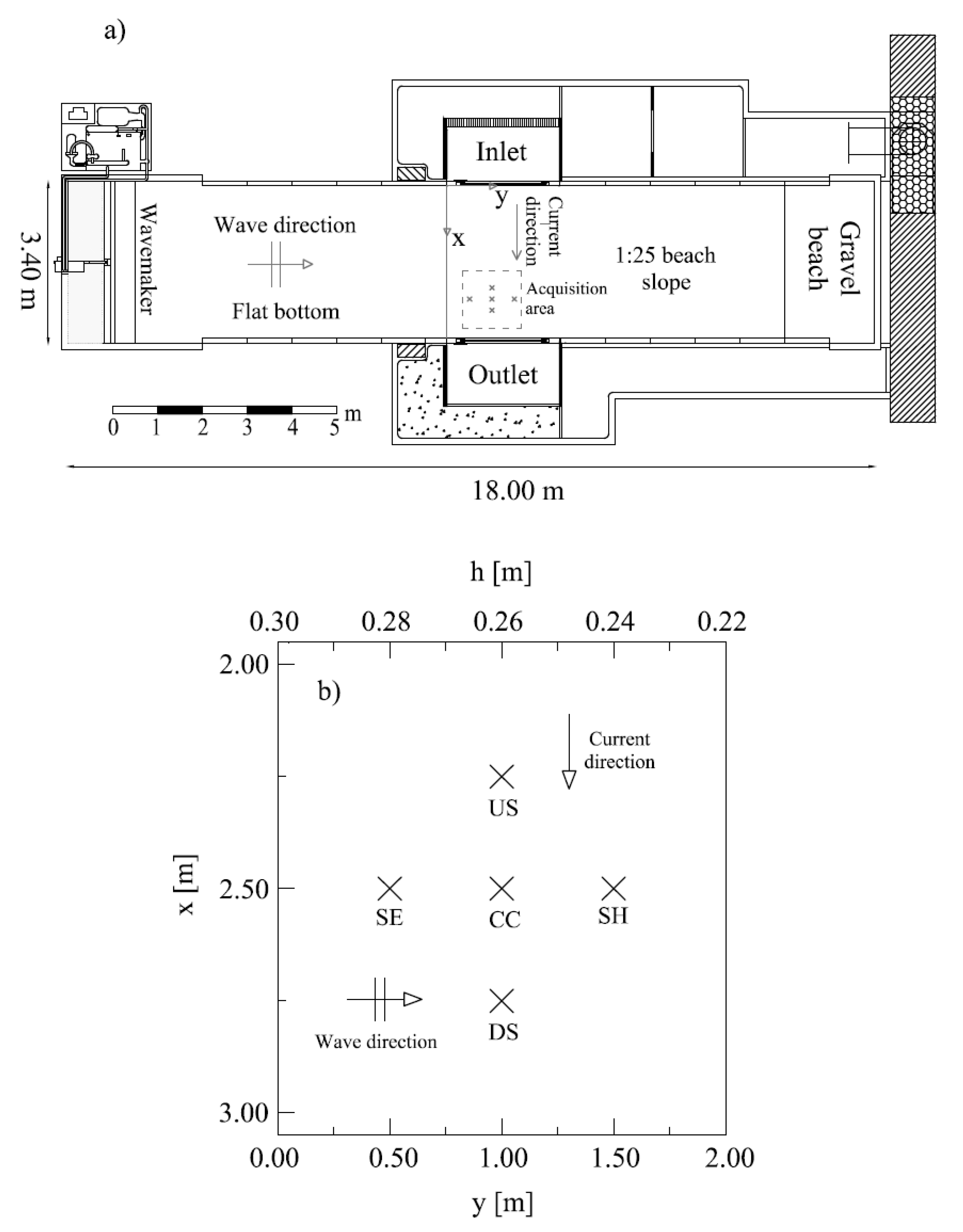
In this section, the results of velocity data analysis are presented and discussed. First, an assessment of the temporal variability of the velocity time-series is shown in order to investigate time variability of the flow field and how it is altered by the presence of the waves. Then, a space variability assessment of the velocity is presented in order to investigate the flow at different positions within the tank. Subsequently, time- and phase-averaged velocity data of CO and WC tests are compared and the results are discussed. In the last subsection turbulent flow is investigated through quadrant analysis.

3.1. Time Variability Assessment

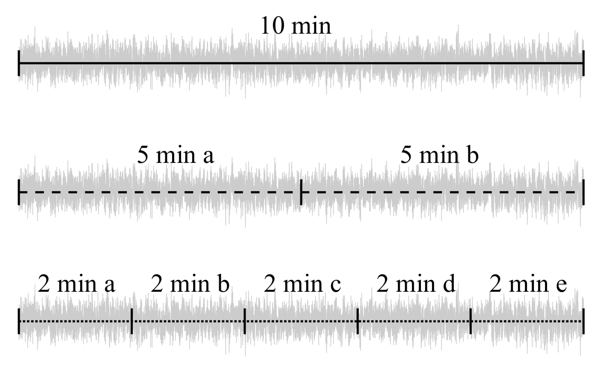
Velocity time series has been subdivided into smaller intervals and then a statistical analysis has been performed in order to assess the time-series variability considering different time spans. Similar approaches have been adopted by [6,21]. Duration of the measured velocity time series is 10 min, which has been divided in 2 segments of 5 min each (called 5 min a, 5 min b) and in 5 segments of 2 min (called 2 min a, 2 min b, 2 min c, 2 min d, 2 min e) as shown in Figure 2.

Dimensionless time-averaged velocities u (=$\overline{u}/U$), v (=$\overline{v}/U$) and w (=$\overline{w}/U$), where $\overline{u}$, $\overline{v}$ and $\overline{w}$ are the dimensional time-averages of $\widehat{u}$, $\widehat{v}$ and $\widehat{w}$, have been computed from the original 10 min time series. The dimensionless time-averaged velocities of the smaller time segments (5 and 2 min) have been computed, namely: $u_{5,s}$, $v_{5,s}$ and $w_{5,s}$, which are the 5 min segment time-averages of the dimensionless streamwise, crosswise and vertical velocity, where s is some specific segment (namely a or b); and $u_{2,s}$, $v_{2,s}$ and $w_{2,s}$, which are the 2 min time-averages of the dimensionless streamwise, crosswise and vertical velocity, where s indicates some specific segment (namely a–e). In order to compare the variability of the different time spans, the deviation of the dimensionless time-averaged velocities computed from a shorter time series compared to the one computed from the entire time series, have been calculated:

$$\Delta u_{10-5s}=u-u_{u,5,s};$$

(5)

$$\Delta u_{10-2s}=u-u_{u,2,s}.$$

(6)

Deviations of the time-averaged velocities for crosswise and vertical velocities are computed as well using the same notation. In a similar way, the variability of the standard deviation has been evaluated as:

$$\Delta {\sigma }_{u,10-5s}={\sigma }_u-{\sigma }_{u,5,s};$$

(7)

$$\Delta {\sigma }_{u,10-2s}={\sigma }_u-{\sigma }_{u,2,s};$$

(8)

where ${\sigma }_u$ is the standard deviation of $\widehat{u}/U$ for the 10 min time series, ${\sigma }_{u,5,s}$ is the standard deviation of the 5 min time series for the segment s (a or b), ${\sigma }_{u,2,s}$ is the standard deviation of the 2 min time series for the segment s (a, b, c, d or e). Standard deviation differences for crosswise and vertical velocities are computed as well using the same notation.

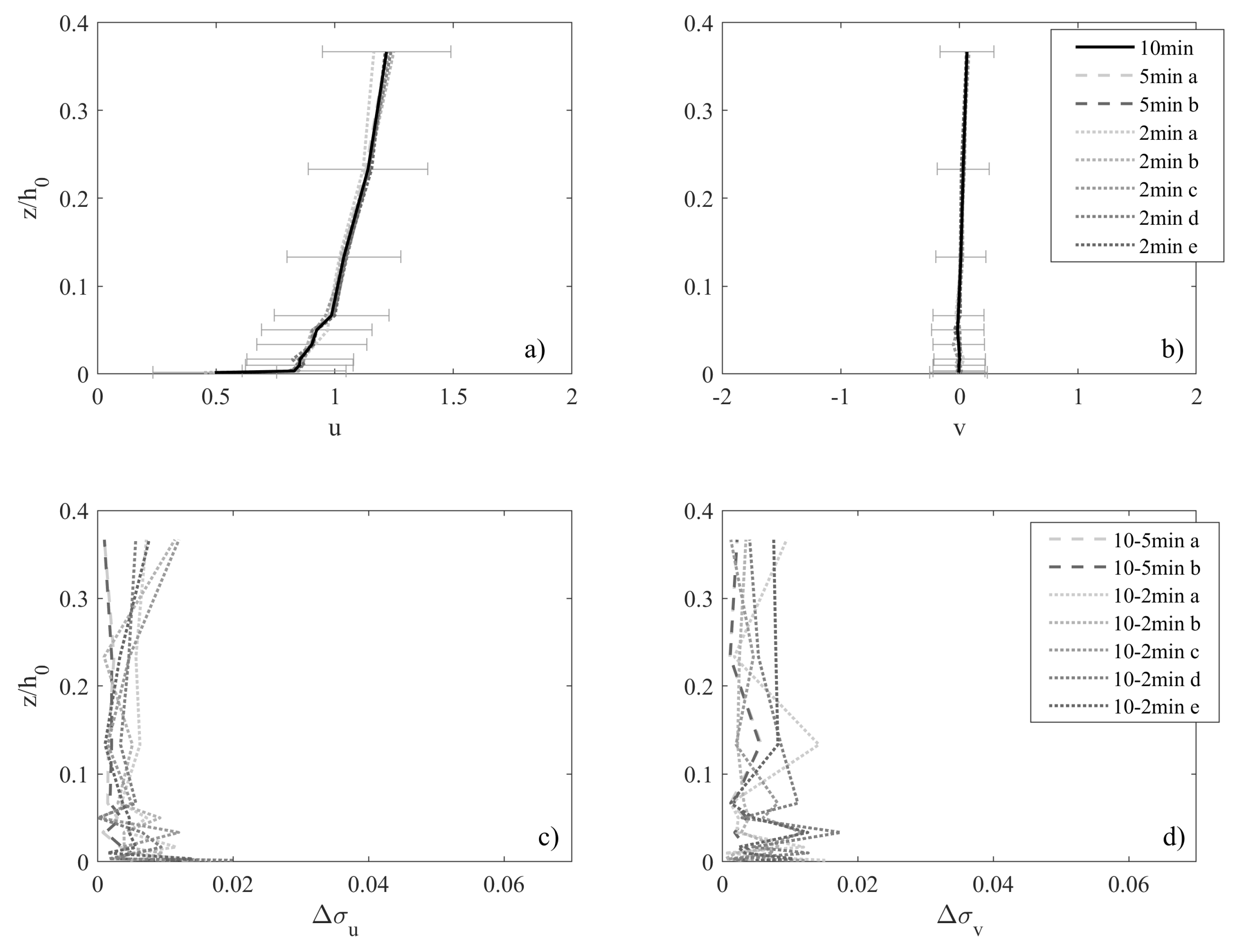
Figure 3 shows the dimensionless time-averaged velocities for test 3 (CC, CO, U = 0.14 m/s) of u (Figure 3a) and v (Figure 3b) for the following timespans: 10 min (continuous line), 5 min (dashed lines), 2 min (dotted lines); error bars indicate standard deviation for the 10 min time series ${\sigma }_u$.

Figure 3a shows that time-averaged velocity profiles are quite similar for all the considered timespans. This suggests that the steadiness of the current is mantained for the entire duration of each experiment even for the smallest examined time segment, with a depth-averaged $\Delta u_{5,s}$ < 0.01, $\Delta u_{2,s}$ < 0.02 and a maximum of 0.06. Standard deviation ${\sigma }_u$ shown by the error bars is quite similar at every measuring position z, with depth-averaged mean of 0.23 (±0.02). The dimensionless time-averaged velocity profiles of v in Figure 3b show a behavior similar to the one of u, with depth-averaged $\Delta v_{5,s}$ < 0.01 and $\Delta v_{2,s}$ < 0.02 and a maximum of 0.05. Standard deviation ${\sigma }_u$ by the error bars is again quite similar at every measuring position z with a depth-averaged value of 0.24 (±0.01). Figure 3c shows the difference of standard deviation of the 10 min time series versus the 5 min one ($\Delta {\sigma }_{u,10-5s}$, dashed line) and the 2 min one ($\Delta {\sigma }_{u,10-2s}$, dotted lines) for test 3 (CO, CC, U = 0.14 m/s) for streamwise (Figure 3c) and crosswise (Figure 3d) velocity. Results indicate that $\Delta {\sigma }_u$ is always below 0.01, with larger deviation peaks observed at the bottom below $z/h_0$ = 0.1. The proximity of the bed may determine local turbulent fluctuations which disappear as a result of the time average as the test duration increases. Nevertheless, the difference between the two 5 min tests is relatively small for all the considered time spans. Standard deviation differences of the crosswise velocity in (Figure 3d) show a very similar behavior, which is below 0.02 all along the water column and for all the time spans.

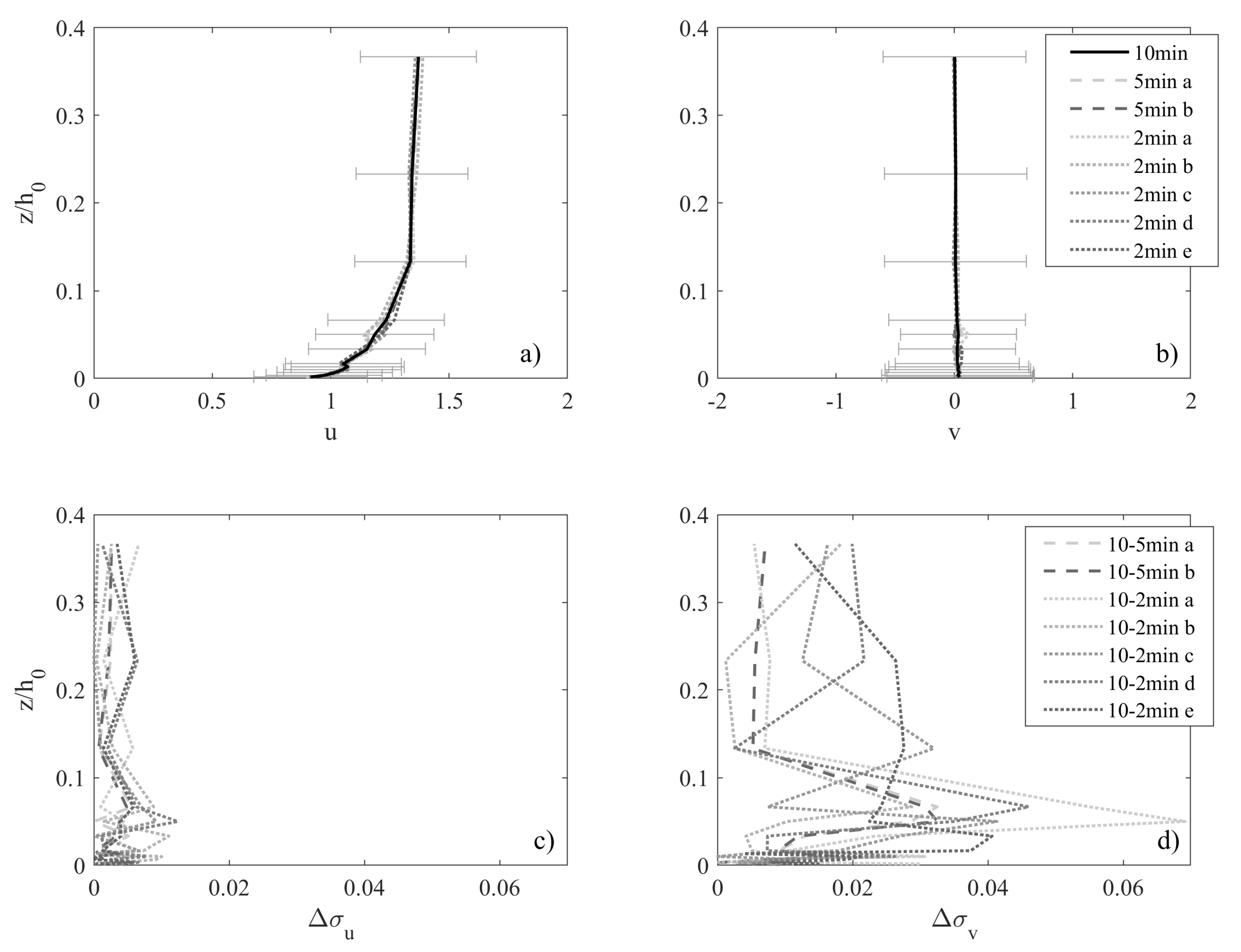
Figure 4 shows the dimensionless time-averaged velocity profiles for test 9 (WC, CC, U = 0.14 m/s) of streamwise (Figure 4a) and crosswise (Figure 4b) velocity for the following time spans: 10 min (continuous line), 5 min (dashed line) and 2 min (dotted line); error bars indicate standard deviation of the 10 min time series. Measuring position and current mean velocity U are the same as test 3, but in test 9 waves are superimposed to the current.

Error bars in Figure 4a shows that the presence of waves does not induce a significant change of long-term variability, since the depth-averaged ${\sigma }_u$ is 0.24 (± 0.01), i.e., equal to the one in the absence of waves. Difference in time-averaged velocity $\Delta u_{5,s}$ and $\Delta u_{2,s}$ are below 0.01 and 0.02 respectively, as for test 3. Figure 4b shows that the presence of the superposed oscillatory motion determines an increase of variability in terms of ${\sigma }_v$ (depth-averaged 0.08 ± 0.01) in comparison with Figure 3b. Variability between time spans $\Delta u$ is, however, lower than the current only case (< 0.01 for both 5 and 2 min time spans), this suggests the occurrence of a wave-induced turbulent momentum transfer from the wave to the current direction. Figure 4 shows standard deviation differences for streamwise (Figure 4c) and crosswise (Figure 4d) velocity profiles for test 9. Comparison between Figure 3c and Figure 4d shows variability between time spans is quite similar to the ones already observed in the current only case. On the other hand, Figure 4d shows instead a significant increase in standard deviation variability between time spans in the crosswise direction, which may reach 0.07 close to the bottom.

3.2. Spatial Variability Assessment

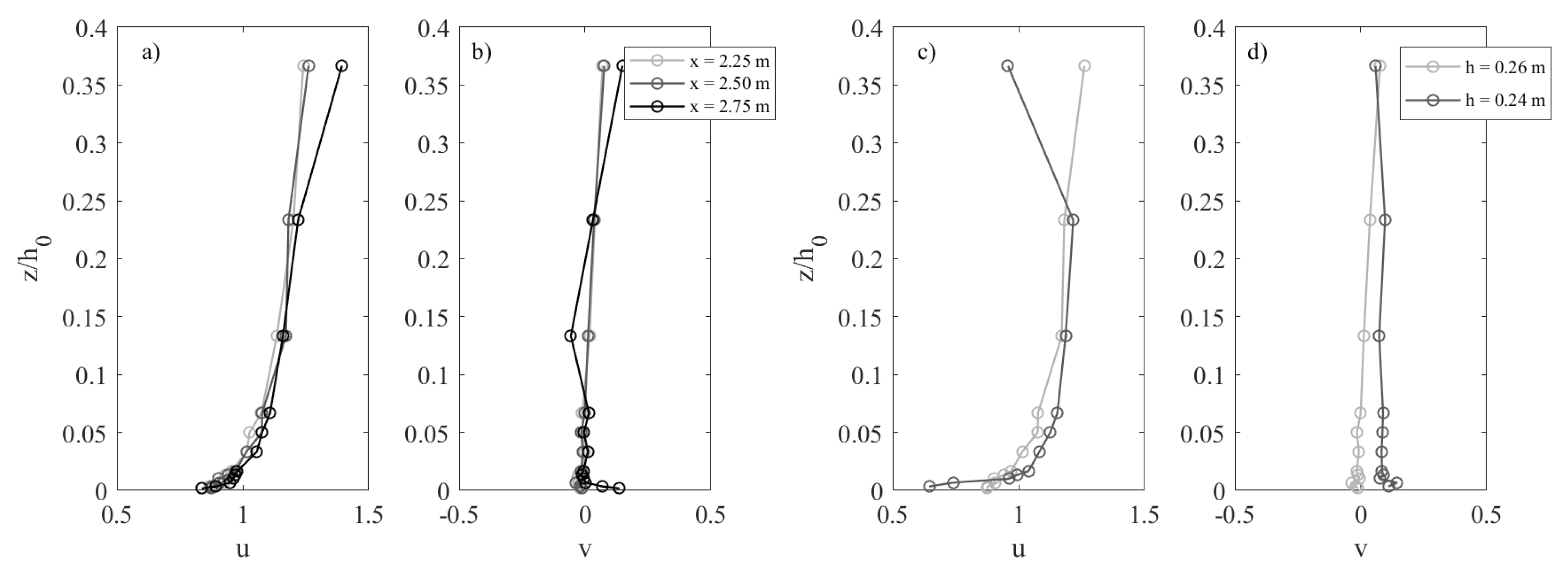
An investigation aimed at studying the flow field at different positions in the wave tank for the CO cases, i.e., at different water depth and along the current, has been performed. Figure 5a,b shows the dimensionless time-averaged u and v velocity profiles in the streamwise and crosswise directions for the CO tests 2, 4 and 5, (CC, US and DS respectively), thus at measuring positions all aligned in the current direction (y = 1.00 m), having the same local water depth h = 0.26 m.

Figure 5a shows that a steady unidirectional current in the x direction is satisfactorily achieved, as the velocity profiles aligned in the x direction have the same velocity distribution along the water column. The upper part of the velocity profile at DS shows an increase in velocity in comparison with the other two positions. As this position is closer to the current outlet, the flow may be affected by the presence of a slightly faster current downstream of the outflow section, which may determine the upper part of the profile to be accelerated. Nevertheless, the depth-averaged difference between dimensionless time-averaged velocities is less than 0.01 of U. Figure 5b shows the dimensionless time-averaged velocity profiles u and v for tests 2 and 6, (CC and SH respectively) thus both aligned in the y direction (x = 2.50 m), with local water depth h = 0.26 m and 0.24 m respectively. Figure 5b shows that u velocity profile of test 6 (SH, h = 0.24 m), which is more shoreward and has a shallower depth in comparison with test 2 (CC, h = 0.26 m), shows a velocity decrease close to the bed and an increase in the central part of the water column. Indeed, as the discharge of the mean current velocity is constant and the local water depth is shallower, the current shows an overall velocity increase as an effect of mass continuity. Due to the increase of velocity, an increased bottom resistance is experienced by the current, which shows a more turbulent velocity distribution in proximity of the bottom, compensated by a velocity increase in the rest of the water column. Velocity profiles of v show that a mean flow directed shoreward is observed all along the water column. This suggests that at the positions shoreward from the central axis of the inflow/outflow sections (y = 1.00 m), a recirculation region may be generated inside the tank, determining the current to veer in the shoreward direction. This veering effect is indeed not observed along the central axis while may reach a maximum value of 10% of U at SH.

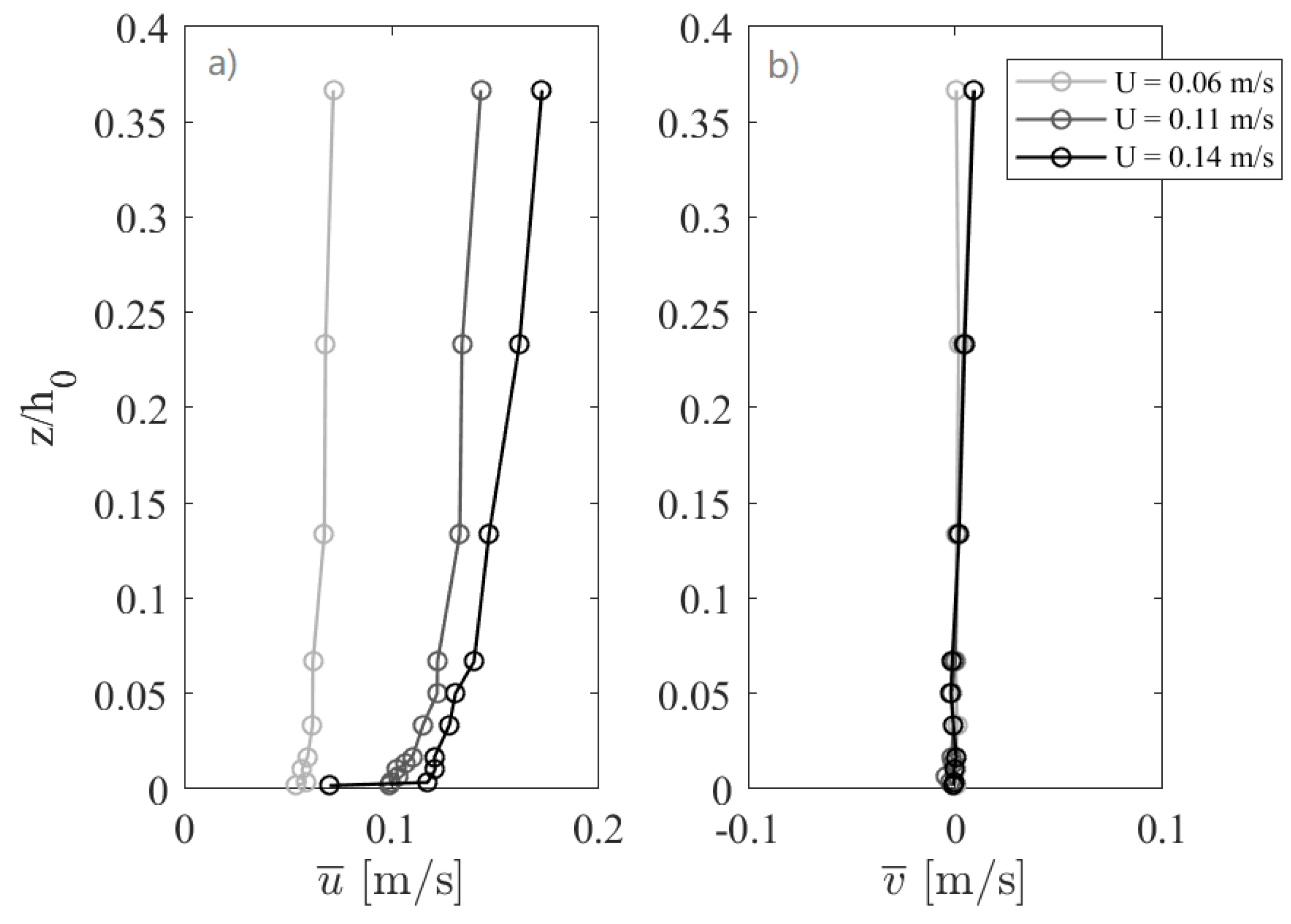
Figure 6 shows the dimensional time-averaged velocities $\overline{u}$ and $\overline{v}$ for CO tests 1, 2 and 3 which are at the same position in the tank (CC) but have different mean current velocity U, equal to 0.06, 0.11 and 0.14 m/s respectively.

It can be observed that the u velocity distribution follows the increase of mean velocity U. The increase of U determines the velocity distribution to be altered, determining progressively larger turbulence-induced flow resistances at the bottom as U increases, showed by the increase of the velocity gradient in the vertical direction. Velocity profiles in the crosswise direction v show values close to zero for all tests along the whole water column, indicating that the current remains unidirectional at y = 1.00 m even with increasing mean current velocity. Moreover, no veering in the crosswise direction is observed, showing that the velocity field at y = 1.00 m (CC, US and DS) is not affected by the recirculation region for all the considered mean current velocities.

3.3. Time- and Phase-Averaged Flow

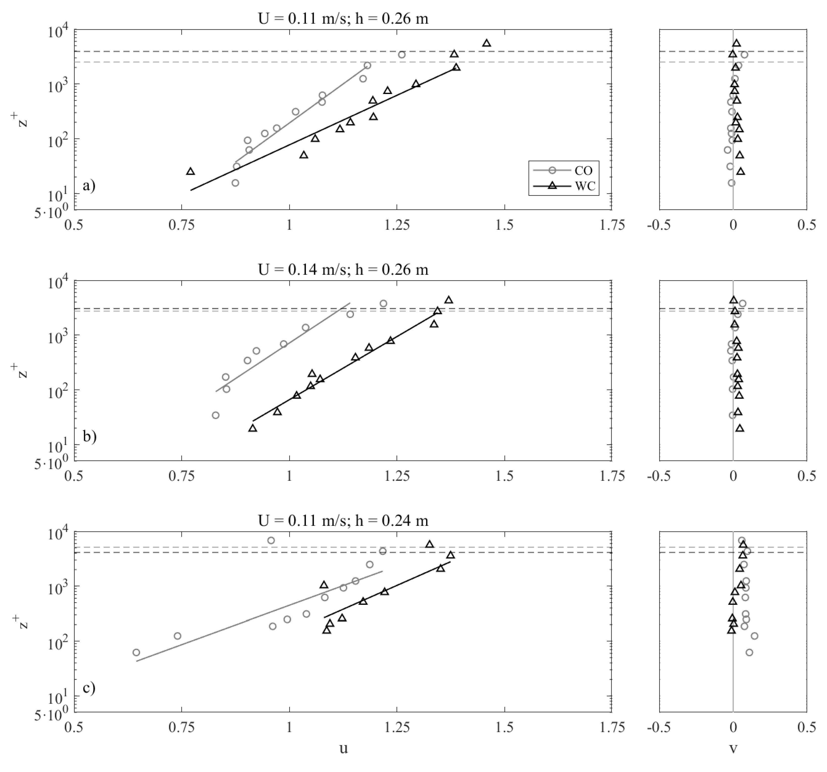
A comparative analysis of CO and WC time- and phase-averaged velocity profiles is carried out in the following, in order to investigate how the mean current flow is affected by the presence of waves. Figure 7a shows the logarithmic profiles of u and v for tests 2 (CO) and 8 (WC), at CC with U = 0.11 m/s. Velocities are plotted versus the dimensionless bed distance $z^{+}=z\nu /u_{\tau }$, where $u_{\tau }$ is the shear velocity. Shear velocity is calculated by the slope of a linear fit of the velocity measurements in the logarithmic profile [30]. Dashed lines indicate the current boundary layer thickness ${\delta }_c$ for the CO (grey) and WC (black) conditions, the continuous line shows the linear fitting of the velocities inside the logarithmic layer.

Figure 7a shows that in comparison with the CO case, the superposition of waves determines a velocity increase along the water column (depth-averaged $\Delta u$ = $u_{WC}-u_{CO}$ = 0.18). This suggests the occurrence of a mean momentum transfer from the wave to the current, thus from the y to the x direction. Moreover, the WC velocity distribution show a more turbulent profile ($u_{\tau }$ = 0.05 m/s) in comparison with the CO case ($u_{\tau }$ = 0.02 m/s), determined by an increase of bottom resistance due to the superposition of the wave boundary layer on the current, which enhances turbulence mixing in the proximity of the bed. Figure 7b shows the logarithmic profiles of u and v for tests 3 (CO) and 9 (WC) with U = 0.14 m/s. Both tests are at CC. The position is the same of tests 2 and 8, whose logarithmic profiles are shown in Figure 7a, but in the presence of a stronger current, a larger transfer of mean momentum in the x direction (depth-averaged $\Delta u$ = 0.30). Moreover, the slopes of the two logarithmic profiles are quite similar ($u_{\tau }$ = 0.03 m/s for the CO case, $u_{\tau }$ = 0.04 m/s for the WC case); in this case, the superposition of waves apparently does not determine an increase in turbulent mixing. Since the sole current is stronger than the case shown in Figure 7a ($R{e}_c$ = 37184 for test 2, $R{e}_c$ = 44857 for test 3), and the wave-current velocity ratio $V_w/U_c$ is slightly smaller ($V_w/U_c$ = 1.36 for test 2, $V_w/U_c$ = 1.17 for test 3), it is possible that the presence of a stronger current inhibits the turbulent mixing induced by the wave motion. Figure 7c shows the logarithmic profiles of u and v for tests 6 (CO) and 12 (WC) with U = 0.11 m/s at SH, thus at a shallower water depth than the tests shown in Figure 7a,b, but with the same U of the test shown in Figure 7a. The presence of waves still determines an overall velocity increase of the current ($\Delta u$ = 0.08) but to a lesser extent than Figure 7a. Similarly to the case of Figure 7b, the superposition of waves does not induce an increase of turbulence in the proximity of the bed ($u_{\tau }$ = 0.05 m/s for test 6, $u_{\tau }$ = 0.06 m/s for test 12). It is possible that, at this condition, as the effect of waves on the water column becomes more relevant as wave shoals ($V_w/U_c$ = 1.71), a partial relaminarization process occur. In other words, the presence of waves may determine a suppression of turbulent mixing. This phenomenon has been already observed by Lodahl et al. [3] when a laminar wave boundary layer is superposed to a current with $V_w/U_c$ > 1. Logarithmic profiles of v in Figure 7c show that the CO case presents a mean flow in the shoreward direction, as an effect of the recirculation flow, as already observed in Section 3.2. Nevertheless, with the waves superposed on the current, this effect is reduced. As the presence of waves determines the generation of an undertow current in the seaward direction, which opposes the above recirculation effect.

Dimensionless phase-averaged current and wave velocities $\tilde{u}$ and $\tilde{v}$ have been computed as follows:

$$\tilde{u}(z,t/T)=\frac{1}{U}\left(\frac{1}{N_w}\sum _{i=1}^{N_w}{u}_i(z,t/T)-\overline{u}\right)$$

(9)

$$\tilde{v}(z,t/T)=\frac{1}{U}\left(\frac{1}{N_w}\sum _{i=1}^{N_w}{v}_i(z,t/T)-\overline{v}\right),$$

(10)

where $N_w$ is the number of waves used for the computation of the phase average. Figure 8 shows the dimensionless phase-averaged velocities $\tilde{u}$ (Figure 8a,b) and $\tilde{v}$ (Figure 8c,d) for tests 9 and 10. The two tests share the water same depth (h = 0.26 m) but have different mean current velocity: U = 0.11 m/s (Figure 8a,c), U = 0.14 m/s (Figure 8b,d) respectively. The wave characteristics are H = 0.085 m, T = 1.0 s.

Figure 8a shows that the presence of waves determines an oscillatory flow to occur in the current direction. During the crest phase, defined as the half-cycle between 0 and 0.5T, a current velocity decrease is observed, whereas during the trough phase, defined as the half-cycle between 0.5T and 1, an increase of velocity of the current is observed. The oscillatory flow in the current direction is found to be out of phase with respect to the wave motion. The phase shift of the crests of $\tilde{u}$ and $\tilde{v}$ can be quantified by the absolute value of the difference between the instant $t/T$ corresponding to the maximum of $\tilde{u}$ and $t/T$ correspondent to the maximum of $\tilde{v}$:

$$\Delta {(t/T)}_{max}=|{(t/T)}_{max\left(\tilde{u}\right)}-{(t/T)}_{max\left(\tilde{v}\right)}|.$$

(11)

Comparison between Figure 8a,b suggests that the presence of a stronger current (U = 0.14 m/s) determines the wave motion to induce a less significant oscillation of $\tilde{u}$, i.e., the amplitude of $\tilde{u}$ is reduced in comparison with the weaker current case. Moreover, phase-averaged current velocities show a smaller phase shift at the bottom in comparison with the rest of the water column (Figure 8b). As current experiences a larger bottom resistance ($u_{\tau }$ = 0.04 m/s) than the case with a weaker current ($u_{\tau }$ = 0.03 m/s, Figure 8a), it is possible that slower parts of the fluid close to the bed are more easily affected by the wave motion, whereas the faster ones in the upper part of the flow may experience a delay.

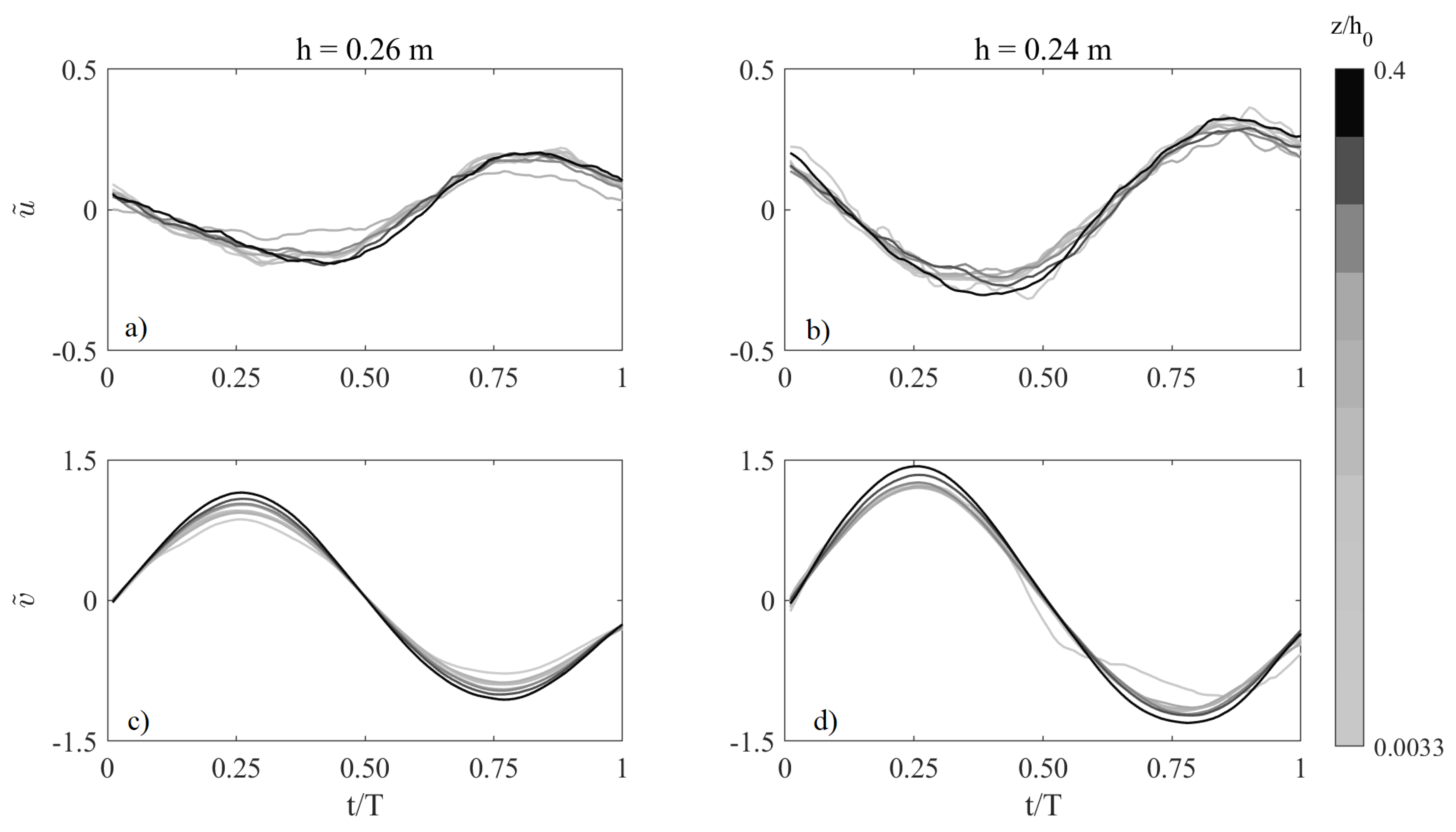
Figure 9 shows the phase-averaged velocities $\tilde{u}$ (Figure 9a,b) and $\tilde{v}$ (Figure 9c,d) for tests 9 and 12, the two tests share the same mean current velocity (U = 0.11 m/s) but measurements were obtained at different water depths: h = 0.26 m (Figure 9a,c), h = 0.24 m Figure (Figure 9b,d) respectively. The wave characteristics are H = 0.085 m, T = 1.0 s.

The data in Figure 9b,d reflect the fact that that wave shoaling is occurring between the two positions (CC and SH, respectively). A larger oscillation is observed as an effect of wave shoaling all along the measured water column. Moreover, a larger phase shift is observed (depth-averaged $\Delta {(t/T)}_{max}$ = 0.60) in comparison with test 9 ($\Delta {(t/T)}_{max}$ = 0.38). A possible explanation is the following: as waves shoal, the wave velocity distribution during a wave phase becomes more skewed, i.e., the absolute value of the wave acceleration during the crest phase increases. On the other hand, as the mean current velocity increases with decreasing depth, the current opposes to the acceleration induced by the wave motion. Indeed, as the momentum carried by the current increases as depth decreases, it is less prone to be affected by the change of velocity induced by the shoaling waves, determining the oscillating effect on the current to be delayed.

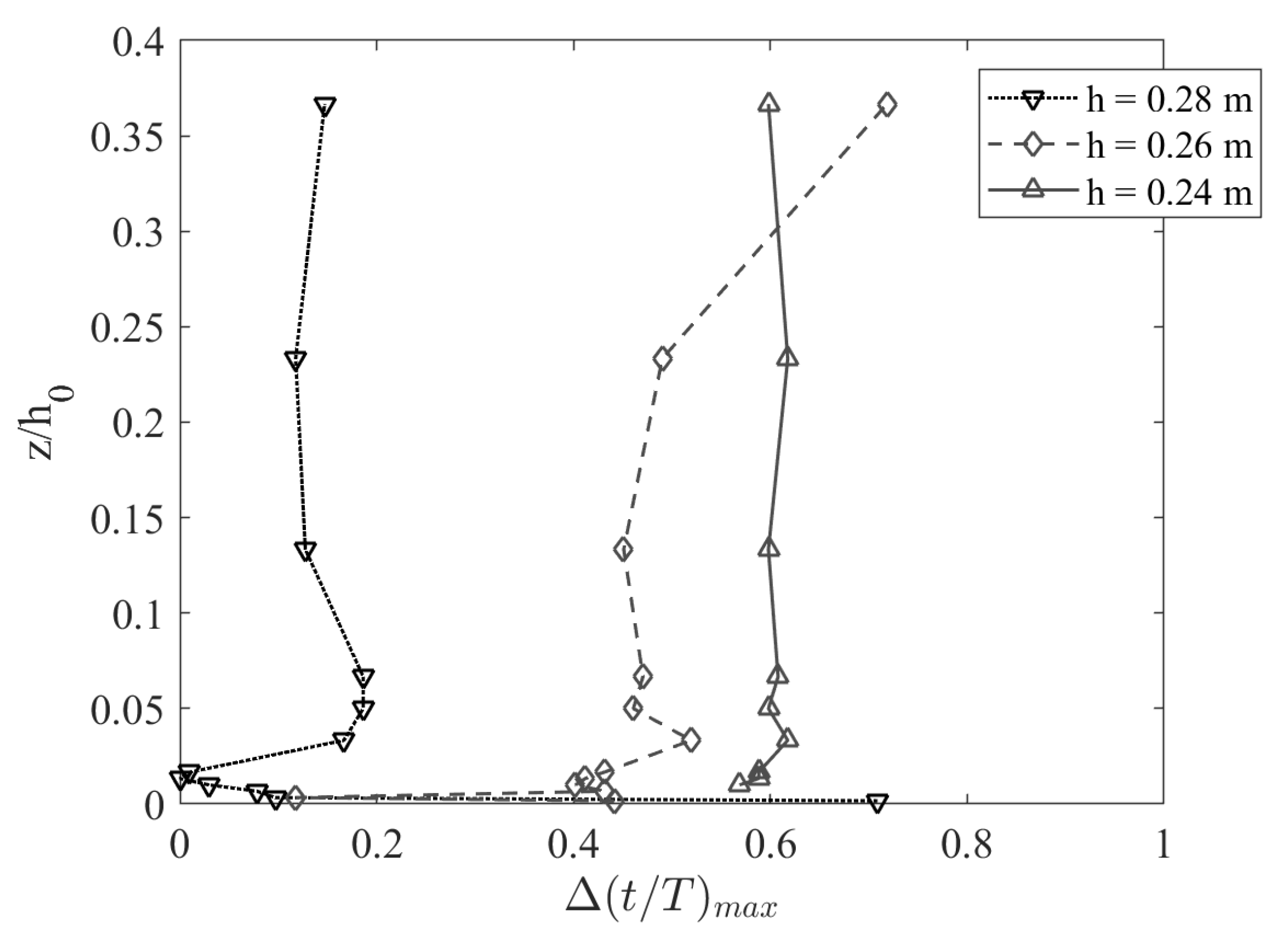
In order to observe how phase shift varies along the water column at different depths, the phase shift profiles of $\Delta {(t/T)}_{max}$ for tests 13, 11 and 12 (h = 0.28 m, 0.26 m and 0.24 m respectively) are shown in Figure 10.

As depth decreases, the depth-averaged phase shift of maximums $\Delta {(t/T)}_{max}$ increases from 0.15 (for h = 0.28 m) to 0.60 (for h = 0.24 m). The current responds to the increasing nonlinearity of the wave velocity distribution with an inertial effect which induces a delay in the phase shift between current and wave oscillations. Moreover, in the lower part of the water column a decrease of phase shift is observed for every $\Delta {(t/T)}_{max}$ profile, although progressively less significant as depth decreases. It can be argued that, as the lower part of the current fluid moves slower, the flow in this region is more prone to move at the same phase of the wave.

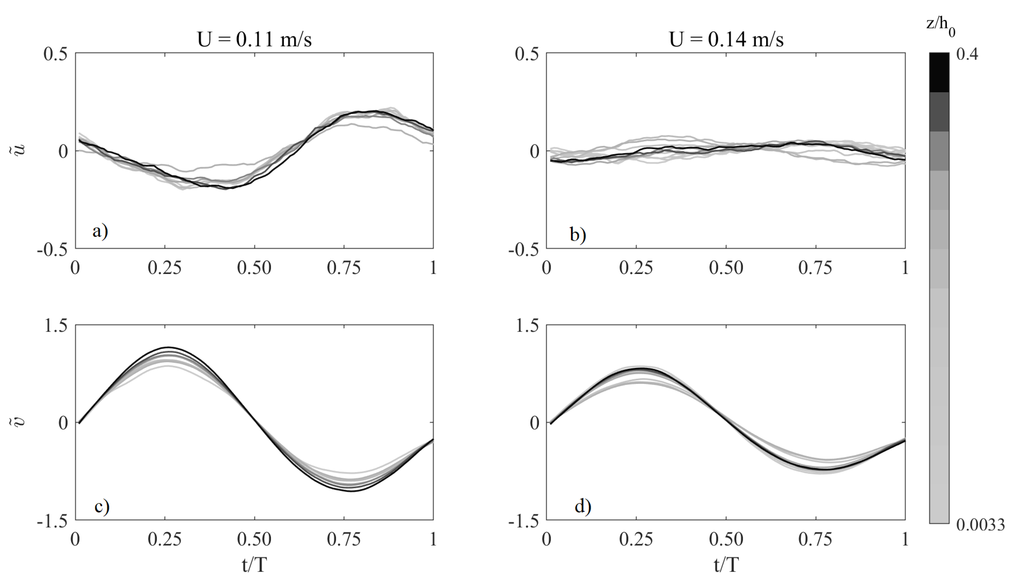
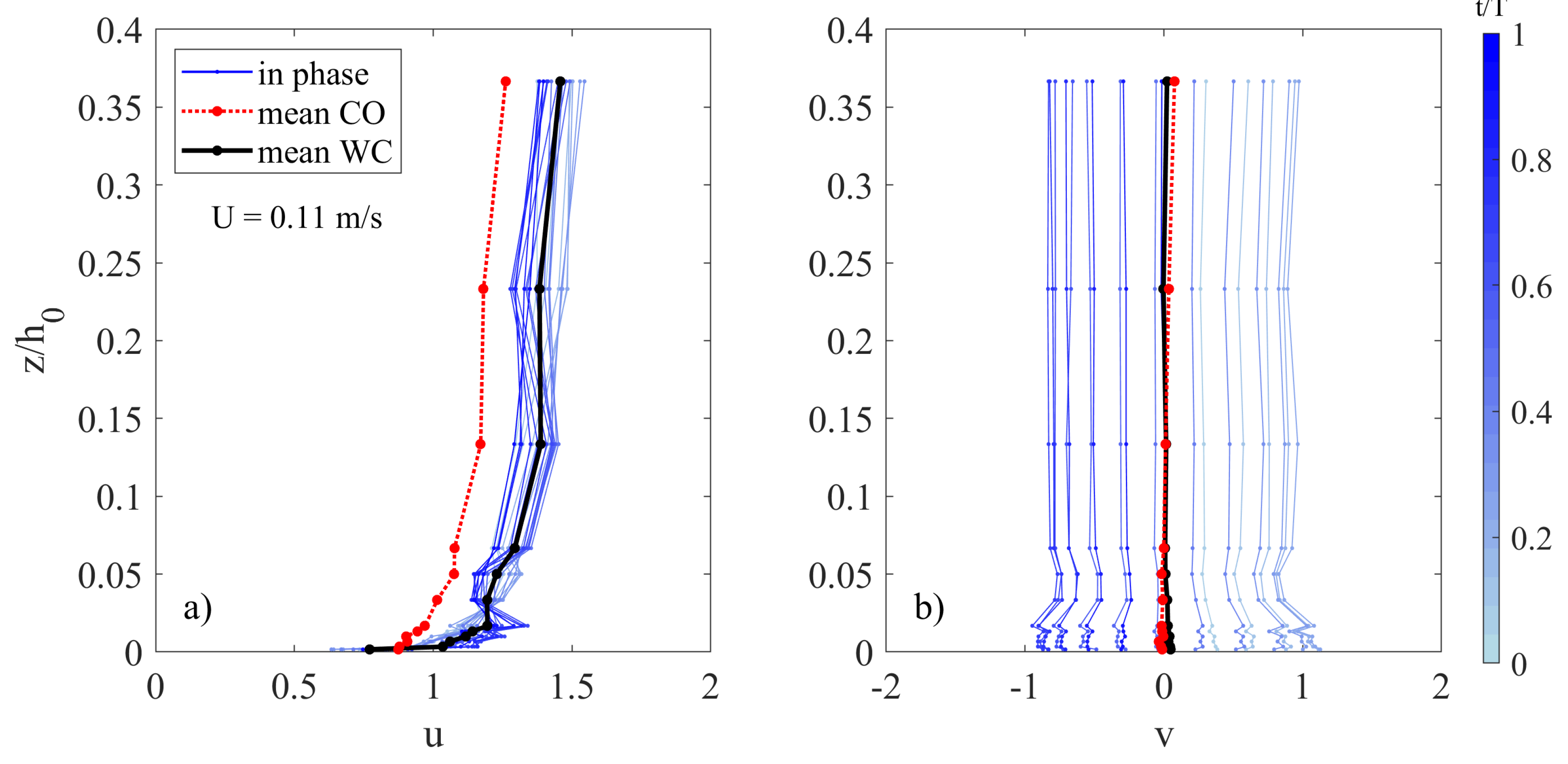
Figure 11 shows the dimensionless phase-averaged and time-averaged velocity profiles for test 8 (WC) and the dimensionless time-averaged velocity profile for test 2 (CO) in the current (Figure 11a) and wave (Figure 11b) direction. Both profiles are measured at the central position and mean current velocity U = 0.11 m/s.

The results indicate that the presence of waves induces current velocities to oscillate around their time-averaged u. The upper part of the velocity profile experiences a decrease in velocity during the crest phase, and an increase of velocity during the trough phase, as already observed in Figure 8 and Figure 9.

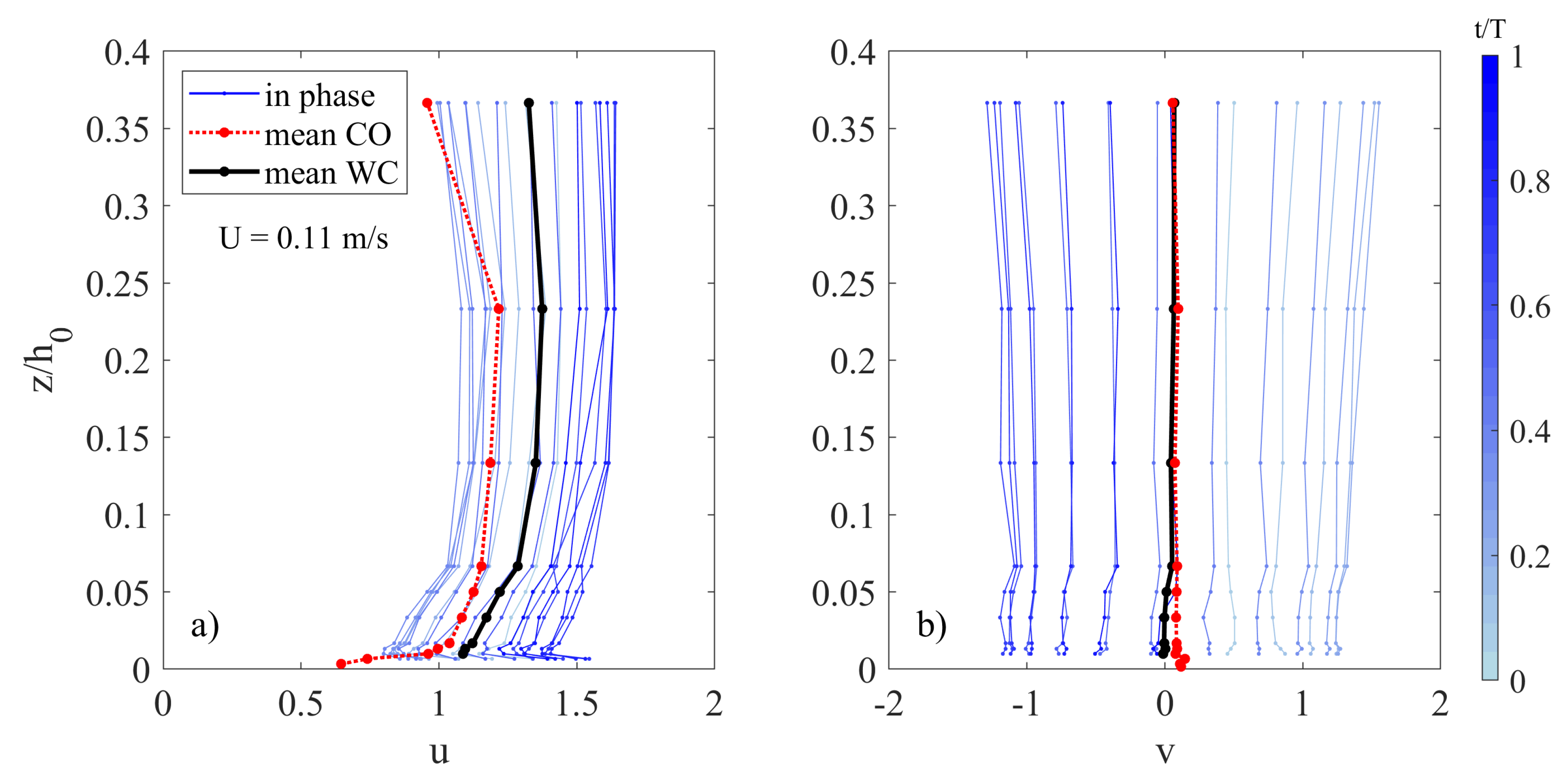
Figure 12 shows the dimensionless phase-averaged and time-averaged velocity profiles for test 12 (WC) and the dimensionless time-averaged velocity profile for test 6 (CO) in the current (Figure 12a) and wave (Figure 12b) direction. Both tests are at shoreward position and mean current velocity U = 0.11 m/s.

By comparing Figure 12a and Figure 11a, a more intense oscillatory motion of the current is determined by the presence of waves, as wave shoaling at this position is determining wave velocity amplitude to increase. This again induces a decrease of velocity during the crest phase and an increase during the trough phase. Such a decrease of velocity forces the current to slow down below the CO measured velocities. Therefore, the current experiences an overall (depth-averaged) velocity increase, but slows down during the crest phase below the CO u profile.

3.4. Turbulent Flow

Wall turbulence manifests with the presence of coherent structures determined by velocity gradients in the boundary layer. Their presence heavily affects mean flow velocity and alters momentum transport, determining an increase of shear resistance. Turbulence production at a wall boundary is generated by the succession of two cyclic events: ejections (or bursts) and sweeps [31]. These events are the main responsible for turbulent vertical momentum transport and they determine the most of the generation of the Reynolds shear stress [32]. Quadrant analysis is a well-established technique to observe the behavior of the ejection-sweep cycle [33,34,35]. Turbulent events, defined as the fluctuating velocities $(u^{\prime }\left(t\right),w^{\prime }\left(t\right))$ of a time series, where $u^{\prime }$ and $w^{\prime }$ are the streamwise and vertical upward turbulent velocities, are subdivided into four quadrants depending on the signs of $u^{\prime }$ and $w^{\prime }$. The first quadrant (Q1), where $u^{\prime }>0$, $w^{\prime }>0$, is called the outward interaction quadrant, the second quadrant (Q2), where $u^{\prime }<0$ and $w^{\prime }>0$, is the ejections quadrant, the third quadrant (Q3), where $u^{\prime }<0$ and $w^{\prime }<0$, is the inward interaction quadrant and the fourth quadrant (Q4), where $u^{\prime }>0$ and $w^{\prime }<0$, is the sweeps quadrant. In a steady flow, the contribution of the i-th quadrant at any point, excluding a hyperbolic region of size $\mathsf{\Omega }$, is

$${\left(u^{\prime }{w}^{\prime }\right)}_{i,\mathsf{\Omega }}=\underset{T\to \infty }{lim}{\int }_0^T{u}^{\prime }\left(t\right)w^{\prime }\left(t\right)I_{i,\mathsf{\Omega }}(u^{\prime },w^{\prime })dt,$$

(12)

where the indicator function $I_{i,\mathsf{\Omega }}$ is

$$I(u^{\prime },w^{\prime })=\left\{\begin{array}{cc}1,\hfill & \mathrm{if}\left(u^{\prime },w^{\prime }\right)\mathrm{is}\mathrm{the}i-\mathrm{th}\mathrm{quadrant}\mathrm{and}\mathrm{if}\hfill \\ & |u^{\prime }{w}^{\prime }|>\mathsf{\Omega }|\overline{u^{\prime }{w}^{\prime }}|\hfill \\ 0,\hfill & \mathrm{otherwise}.\hfill \end{array}\right.$$

In particular, $\mathsf{\Omega }$ is a threshold parameter which allows to consider as ejections-sweep events only the values of $\left(u^{\prime }{w}^{\prime }\right)$ that are larger than $\mathsf{\Omega }$ times $|\overline{u^{\prime }{w}^{\prime }}|$. The threshold parameter is used to observe the relative importance of the quadrant events in generating significantly strong shear stress.

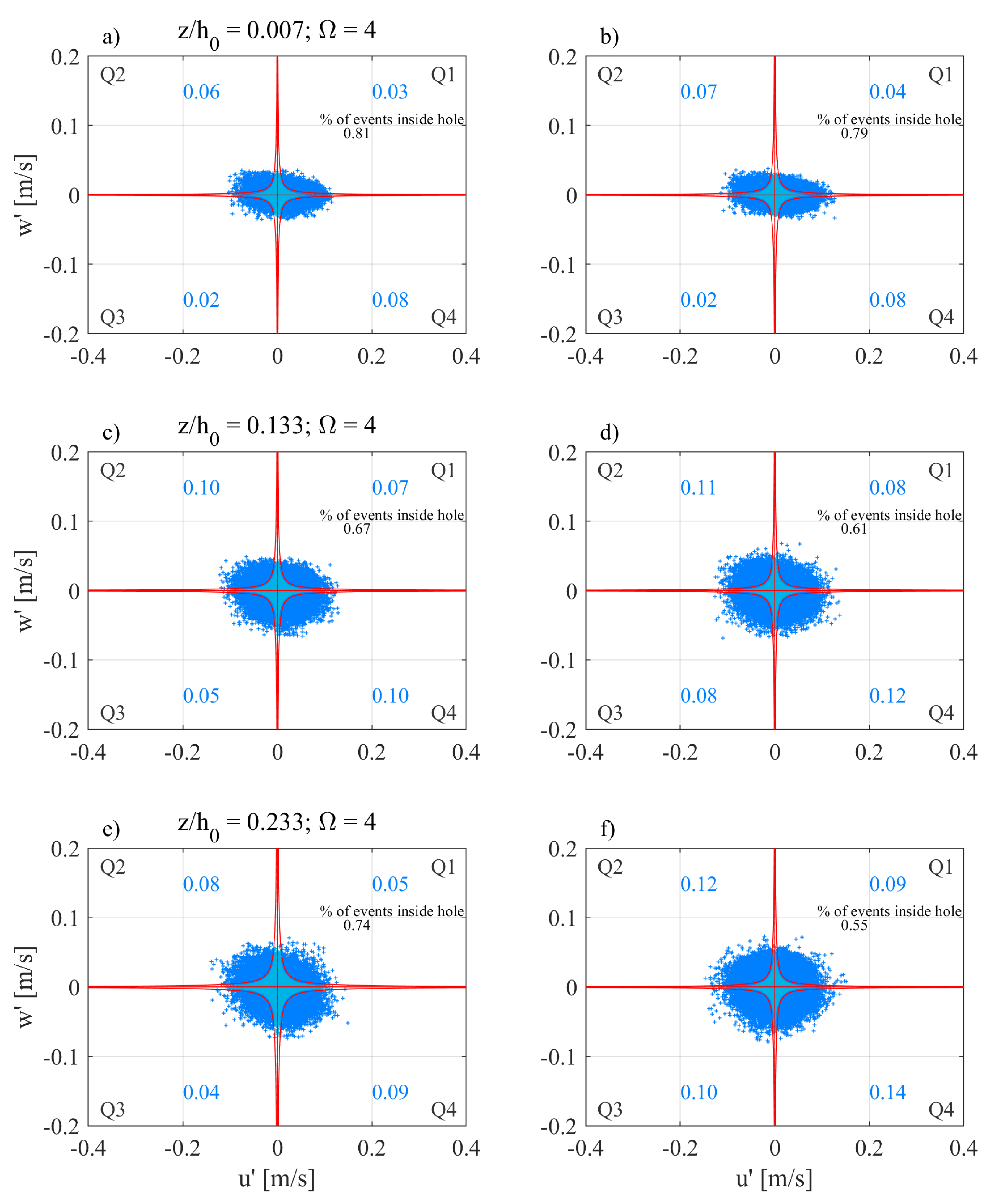
Figure 13a,c,e shows the correlation plots for $u^{\prime }$ and $w^{\prime }$ for test 3 (CO, CC, U = 0.14 m/s) whereas Figure 13b,d,f shows the correlation plots for test 9 (WC, CC, U = 0.14 m/s), at different distances from the bottom: $z/h_0$ = 0.007 (Figure 13a,b), $z/h_0$ = 0.133 (Figure 13c,d), $z/h_0$ = 0.233 (Figure 13e,f). The percentage of events occurring in each quadrant are indicated (light blue), excluding a central hyperbolic region with threshold $\mathsf{\Omega }|\overline{u^{\prime }{w}^{\prime }}|$. The study has been carried out by varying the threshold parameter $\mathsf{\Omega }$, although in Figure 13 only the hole region with $\mathsf{\Omega }$ = 4 is shown.

Comparison between CO (Figure 13a,c,e) and WC (Figure 13b,d,f) shows that, at every considered $z/h_0$ an increase in the relative number of ejection events is always observed when waves are added. This suggests that the presence of waves enhances turbulent mixing all along the water column. In the lower part of the water column (Figure 13e,f) the overall shape of the correlation plot is fairly elliptical in the direction of the Q2 and Q4 quadrants. This suggests that turbulent events distribution is skewed in the direction of the Q2 and Q4, showing that turbulent momentum transfer at the wall is mainly driven by ejection (Q2) and sweep (Q4) events, only a slight difference can be observed between CO and WC case. As distance from bottom increases (Figure 13c,d) the overall shape of the turbulent events overall shape turns from elliptical to almost circular. Turbulent events relatively diminishes in the Q2 and Q4 quadrants in favor of quadrants Q1 and Q3. The turbulent momentum transfer progressively leaves the ejections-sweeps cycle as a main mechanism of turbulent mixing to a more isotropic behavior. The presence of waves enhances turbulent ejections, but also outward and inward interactions. Moreover, the hole region associated with the Reynolds stress $|\overline{u^{\prime }{w}^{\prime }}|$ decreases in size, and the number of events inside the hole decreases likewise. In the upper part of the water column (Figure 13e,f) turbulent events distribution is even less elliptical. Here, the presence of waves determines an overall increase of turbulent fluctuations in all quadrants. Moreover, the presence of waves leads to a smaller Reynolds stress value, as the hyperbolic threshold is lower in the WC case.

4. Conclusions

In the present work an experimental investigation on shoaling waves interacting at a right angle with a current has been carried out. The study aimed to investigate how the hydrodynamic field of a steady current is affected by the superposition of orthogonal waves which progressively shoals over a planar beach. A series of experiments have been conducted in an experimental wave tank, where waves were superposed on an orthogonal current over a 1:25 sloping concrete beach. Surface elevation and flow velocities in the current, wave and vertical directions have been recovered by means of resistive gauges and an Acoustic Doppler Velocimeter respectively. Measured velocity time series have been processed in order to compute time-, phase-averaged and fluctuating velocities and investigate mean, phase and turbulent flow field. A preliminary analysis has been carried out in order to assess the time variability of the flow field within the experimental tank. Results showed that, in the presence of a sole current, steady flow conditions are satisfactorily achieved, and the variability, in terms of difference of standard deviation, of the smallest acquisition time (2 min) did not exceed 2%. The presence of waves determines an increase in the time variability in the wave direction, with a maximum difference of standard deviation of 7% for the 2 min long time series. The following data analysis have been then carried out time-averaging the whole 10 min time series, in which the difference of standard deviation is below 2% for both CO and WC cases. Spatial characterization of the flow field for the sole current has been conducted in order observe how the current velocity profile is altered by the presence of the sloping bed. Vertical velocity profiles showed slight differences between the measured velocities close to the inflow/outflow central axis, nevertheless a mean flow is observed in the shoreward direction farther from the central axis. This suggests the presence of a recirculation region, which conveys part of the current away from the outlet. However, such a recirculation region does not seem to affect the flow field close to the inlet/outlet central axis. Moreover, the space variability analysis showed that as local depth decreases in the shoreward direction, current velocity distribution features a more turbulent profile along with an increase of $R{e}_c$.

The data analysis of the time- and phase-averaged flow showed a complex interaction between the shoaling waves and the steady current in terms of sheer production, momentum transfer and turbulent mixing. A comparison between CO and WC experiments showed that the superposition of waves determines the current to experience a larger shear at the bottom, which suggests the occurrence of an enhanced turbulent mixing induced by the oscillatory motion. Conversely, the upper part of the measured profile experiences a velocity increase. As waves shoal a mean momentum transfer in the upper part of the flow is observed as well, however, the presence of waves does not seem to enhance significantly turbulent shear. A possible explanation is that, in the presence of a current with a larger $R{e}_c$, wave motion may be less effective in inducing an increase of turbulent mixing. Analysis of phase-averaged velocities showed that the superposition of waves induces the current to oscillate around its mean velocity. Moreover, a phase shift between current and wave phase-averaged velocity maximums has been observed. Such a phase shift seems to be enhanced gradually as the waves shoal. Indeed, as waves shoal, wave acceleration increases during the crest phase and velocity amplitude increases as well. On the other hand, the mean current velocity increases with decreasing depth, carrying a larger momentum along its direction. Therefore, while shoaling waves induce the amplitude of the current oscillation to increase, a larger momentum current opposes to the wave increased acceleration, determining the occurrence of a delay in the oscillatory motion of the current. Quadrant analysis applied to turbulent flow showed that the presence of waves induces an increase of the ejection-sweep cycle events, which determines turbulent mixing to be enhanced. Moving farther from the bottom, turbulent field progressively abandon the ejection-sweep cycle as the main mechanism of turbulent momentum transfer, in favour of a more isotropic turbulence mixing.

References

1. Kemp, P.; Simons, R. The interaction between waves and a turbulent current: Waves propagating with the current. J. Fluid Mech. 1982, 116, 227–250. [Google Scholar] [CrossRef] [Green Version]
2. Kemp, P.; Simons, R. The interaction of waves and a turbulent current: Waves propagating against the current. J. Fluid Mech. 1983, 130, 73–89. [Google Scholar] [CrossRef] [Green Version]
3. Lodahl, C.; Sumer, B.M.; Fredsøe, J. Turbulent combined oscillatory flow and current in a pipe. J. Fluid Mech. 1998, 373, 313–348. [Google Scholar] [CrossRef]
4. Thomas, G. Wave–current interactions: An experimental and numerical study. Part 2. Nonlinear waves. J. Fluid Mech. 1990, 216, 505–536. [Google Scholar] [CrossRef]
5. Yuan, J.; Madsen, O.S. Experimental and theoretical study of wave–current turbulent boundary layers. J. Fluid Mech. 2015, 765, 480–523. [Google Scholar] [CrossRef]
6. Mathisen, P.P.; Madsen, O.S. Waves and currents over a fixed rippled bed: 1. Bottom roughness experienced by waves in the presence and absence of currents. J. Geophys. Res. Ocean. 1996, 101, 16533–16542. [Google Scholar] [CrossRef]
7. Fredsøe, J.; Andersen, K.H.; Sumer, B.M. Wave plus current over a ripple-covered bed. Coast. Eng. 1999, 38, 177–221. [Google Scholar] [CrossRef]
8. Grant, W.D.; Madsen, O.S. Combined wave and current interaction with a rough bottom. J. Geophys. Res. Ocean. 1979, 84, 1797–1808. [Google Scholar] [CrossRef]
9. Fredsøe, J. Turbulent boundary layer in wave-current motion. J. Hydraul. Eng. 1985, 110, 1103–1120. [Google Scholar] [CrossRef]
10. Huang, Z.; Mei, C.C. Effects of surface waves on a turbulent current over a smooth or rough seabed. J. Fluid Mech. 2003, 497, 253–287. [Google Scholar] [CrossRef]
11. Johnson, H.K.; Karambas, T.V.; Avgeris, I.; Zanuttigh, B.; Gonzalez-Marco, D.; Caceres, I. Modelling of waves and currents around submerged breakwaters. Coast. Eng. 2005, 52, 949–969. [Google Scholar] [CrossRef]
12. Olabarrieta, M.; Medina, R.; Castanedo, S. Effects of wave-current interaction on the current profile. Coast. Eng. 2010, 57, 643–655. [Google Scholar] [CrossRef]
13. Fernando, P.C.; Guo, J.; Lin, P. Wave–current interaction at an angle 1: Experiment. J. Hydraul. Res. 2011, 49, 424–436. [Google Scholar] [CrossRef]
14. Davies, A.; Soulsby, R.; King, H. A numerical model of the combined wave and current bottom boundary layer. J. Geophys. Res. Ocean. 1988, 93, 491–508. [Google Scholar] [CrossRef]
15. Mao, M.; Xia, M. Dynamics of wave–current–surge interactions in Lake Michigan: A model comparison. Ocean Model. 2017, 110, 1–20. [Google Scholar] [CrossRef] [Green Version]
16. Mao, M.; Xia, M. Wave–current dynamics and interactions near the two inlets of a shallow lagoon–inlet–coastal ocean system under hurricane conditions. Ocean Model. 2018, 129, 124–144. [Google Scholar] [CrossRef]
17. Marino, M.; Faraci, C.; Musumeci, R. An experimental setup for combined wave-current flow interacting at a right angle over a plane beach. Ital. J. Eng. Geol. Environ. 2020. submitted. [Google Scholar]
18. Musumeci, R.; Cavallaro, L.; Foti, E.; Scandura, P.; Blondeaux, P. Waves plus currents crossing at a right angle: Experimental investigation. J. Geophys. Res. Ocean. 2006, 111. [Google Scholar] [CrossRef]
19. Faraci, C.; Foti, E.; Musumeci, R. Waves plus currents at a right angle: The rippled bed case. J. Geophys. Res. Ocean. 2008, 113. [Google Scholar] [CrossRef] [Green Version]
20. Faraci, C.; Scandura, P.; Musumeci, R.; Foti, E. Waves plus currents crossing at a right angle: Near-bed velocity statistics. J. Hydraul. Res. 2018, 56, 464–481. [Google Scholar] [CrossRef] [Green Version]
21. Lim, K.Y.; Madsen, O.S. An experimental study on near-orthogonal wave–current interaction over smooth and uniform fixed roughness beds. Coast. Eng. 2016, 116, 258–274. [Google Scholar] [CrossRef]
22. Marino, M.; Rabionet, I.; Musumeci, R.; Foti, E. Reliability of pressure sensors to measure wave height in the shoaling region. Coast. Eng. Proc. 2018, 36, 10. [Google Scholar] [CrossRef] [Green Version]
23. De Serio, F.; Mossa, M. A laboratory study of irregular shoaling waves. Exp. Fluids 2013, 54, 1536. [Google Scholar] [CrossRef]
24. Faraci, C.; Scandura, P.; Foti, E. Reflection of sea waves by combined caissons. J. Waterw. Port Coast. Ocean Eng. 2014, 141, 04014036. [Google Scholar] [CrossRef]
25. Svendsen, I.A. Introduction to Nearshore Hydrodynamics; World Scientific: Singapore, 2006; Volume 24. [Google Scholar]
26. Schlichting, H. Boundary Layer Theory; McGraw Hill Book Co.: New York, NY, USA, 1968. [Google Scholar]
27. Sleath, J. Turbulent oscillatory flow over rough beds. J. Fluid Mech. 1987, 182, 369–409. [Google Scholar] [CrossRef]
28. Wahl, T.L. Analyzing ADV data using WinADV. In Proceedings of the ASCE Joint Conference on Water Resources Engineering and Water Resources Planning and Management, Minneapolis, MN, USA, 30 July–2 August 2000; pp. 1–10. [Google Scholar]
29. Goring, D.G.; Nikora, V.I. Despiking acoustic Doppler velocimeter data. J. Hydraul. Eng. 2002, 128, 117–126. [Google Scholar] [CrossRef] [Green Version]
30. Sumer, B. Lecture Notes on Turbulence: Revised/Updated 2013; Technical Univ. of Denmark: Lyngby, Denmark, 2007. [Google Scholar]
31. Corino, E.R.; Brodkey, R.S. A visual investigation of the wall region in turbulent flow. J. Fluid Mech. 1969, 37, 1–30. [Google Scholar] [CrossRef] [Green Version]
32. Wallace, J.M. Quadrant Analysis in Turbulence Research: History and Evolution. Annu. Rev. Fluid Mech. 2016, 48, 131–158. [Google Scholar] [CrossRef]
33. Wallace, J.M.; Eckelmann, H.; Brodkey, R.S. The wall region in turbulent shear flow. J. Fluid Mech. 1972, 54, 39–48. [Google Scholar] [CrossRef]
34. Lu, S.S.; Willmarth, W.W. Measurements of the structure of the Reynolds stress in a turbulent boundary layer. J. Fluid Mech. 1973, 60, 481–511. [Google Scholar] [CrossRef]
35. Kim, J.; Moin, P.; Moser, R. Turbulence statistics in fully developed channel flow at low reynolds number. J. Fluid Mech. 1987, 177, 133–166. [Google Scholar] [CrossRef] [Green Version]
Figure 1. (a) Experimental tank for wave-current interaction; (b) top-view of the acquisition area.
Jmse 08 00281 g001
Figure 2. Subdivision in time segments of the original 10 min time series.
Jmse 08 00281 g002
Figure 3. Mean velocity time variability for test 3 (CO, CC, U = 0.14 m/s): Dimensionless time-averaged velocity profiles with the different timespans for streamwise (a) and crosswise (b) velocities, standard deviation differences from the 10 min timespan expressed as a fraction of U for streamwise (c) and crosswise (d) velocities.
Jmse 08 00281 g003
Figure 4. Mean velocity time variability for test 9 (WC, CC, U = 0.14 m/s): dimensionless time-averaged velocity profiles with the different timespans for streamwise (a) and crosswise (b) velocities, standard deviation different from the 10 min timespan expressed as a fraction of U for streamwise (c) and crosswise (d) velocities.
Jmse 08 00281 g004
Figure 5. Dimensionless time-averaged u and v velocity profiles in the streamwise and crosswise directions: velocity profiles of u (a) and v (b) for the CO tests 2, 4 and 5, (CC, US and DS respectively) thus all aligned in the x direction (y = 1.00 m) having the same local water depth h = 0.26 m; velocity profiles of u (c) and v (d) for tests 2 and 6, (CC and SH respectively) thus both aligned in the y direction (x = 2.50 m) with local water depth of h = 0.26 m and 0.24 m respectively.
Jmse 08 00281 g005
Figure 6. Dimensional time-averaged velocity profiles u ¯ (a) and v ¯ (b) directions for tests 1, 2 and 3 (CO). All the tests have the same position (CC, h = 0.26 m) but different U.
Jmse 08 00281 g006
Figure 7. Dimensionless time-averaged logarithmic velocity profiles in the streamwise and crosswise direction: (a) tests 2 (CO) and 8 (WC) at CC with U = 0.11 m/s; (b) tests 3 (CO) and 9 (WC) at CC with U = 0.14 m/s; (c) tests 6 (CO) and 12 (WC) at SH with U = 0.11 m/s. All the tests are at CC (x = 2.50 m, y = 1.00 h = 0.26 m). Dashed lines indicate the current boundary layer thickness δ c for the CO (grey) and WC (black) cases.
Jmse 08 00281 g007
Figure 8. Phase-averaged velocities for tests 9 and 10 (WC, H = 0.085 m, T = 1.0 s) in the crosswise (a,b) and streamwise (c,d) direction. Both tests have the same local water depth h = 0.26 m but different mean current velocity: U = 0.11 m/s (a,c) and U = 0.14 m/s (b,d).
Jmse 08 00281 g008
Figure 9. Phase-averaged velocities for tests 9 and 10 (WC, H = 0.085 m, T = 1.0 s) in the crosswise (a,b) and streamwise (c,d), with local water depth h = 0.26 m (a,c) and h = 0.24 m (b,d): U = 0.11 m/s (a,c) and U = 0.14 m/s (b,d).
Jmse 08 00281 g009
Figure 10. Phase shift between maximums of phase-averaged velocities u ˜ and v ˜ .
Jmse 08 00281 g010
Figure 11. Phase-averaged velocities for tests 2 and 8 (CO and WC respectively) in the streamwise (a) and crosswise (b) directions. Time-averaged CO profile (red dashed line, red dot marker), time-averaged WC profile (black thick continuous line, black dot marker) and phase-averaged WC profile (see color bar). Mean velocity U = 0.11 m/s, local water depth h = 0.26 m.
Jmse 08 00281 g011
Figure 12. Phase-averaged velocities for tests 6 and 12 (CO and WC respectively) in the streamwise (a) and crosswise (b) directions. Time-averaged CO profile (red dashed line, red dot marker), time-averaged WC profile (black thick continuous line, black dot marker) and phase-averaged WC profile (see color bar). Mean velocity U = 0.11 m/s, local water depth h = 0.24 m.
Jmse 08 00281 g012
Figure 13. Correlation plots for u and w for test 3 (CO, a,c,e) and test 9 (WC, b,d,f), at different distance from bottom: z / h 0 = 0.007 (a,b), z / h 0 = 0.133 (c,d), z / h 0 = 0.233 (e,f). Both tests are at central position and have same mean current velocity U = 0.14 m/s. Hyperbolic hole Ω = 4.
Jmse 08 00281 g013