Steady Streaming Induced by Asymmetric Oscillatory Flows over a Rippled Bed

Abstract

The flow induced by progressive water waves propagating over a rippled bed is reproduced by means of the numerical solution of momentum and continuity equations to gain insights on the steady streaming induced in the bottom boundary layer. When the pressure gradient that drives the flow is given by the sum of two harmonic components an offshore steady streaming is generated within the boundary layer which persists in the irrotational region. This steady streaming depends on the Reynolds number and on the geometrical characteristics of the ripples. Nothwithstanding the presence of a steady velocity component, the time-average of the force on the ripples vanishes.

1. Introduction

The knowledge of the flow induced by surface waves close the bottom of the sea is important to predict the vertical distribution of the wave induced velocity and to formulate reliable models of sediment transport. One of the most important characteristics of the boundary layer at the bottom of sea waves is the generation of a steady velocity component induced by the nonlinearity of momentum equation. The existence of this steady streaming was first highlighted by [1] and then it was theoretically explained by [2] for waves propagating over a horizontal flat bed, when the flow regime in the bottom boundary layer is laminar. In particular, Ref. [2] showed that, close to the bed, but outside the boundary layer, a mean onshore velocity of magnitude $0.75U_0^{*2}/c^{*}$ is present, where $c^{*}$ is the wave speed and $U_0^{*}$ is the amplitude of the velocity oscillations near the bed. This streaming is due to the mean Reynolds stress generated because of the non-uniform distribution of the velocity in the boundary layer along the longitudinal extension of the surface wave. In the mean moment equation, the vertical gradient of this mean Reynolds stress consists of a force applied to the fluid particles which is balanced by the viscous stress associated with a steady streaming.

As discussed by [2], the profile of the steady velocity component in the core region is significantly affected by the steady streaming induced in the bottom boundary layer that plays the role of the boundary condition for the flow in the core region.

More recent studies have shown that the direction (onshore/offshore) and the intensity of the steady streaming close to the sea bed is affected by turbulence dynamics when asymmetric or skewed waves are present [3,4,5,6]. Even in this case, the streaming is affected by non-vanishing mean values of the Reynolds stress, but the mechanism generating this mean stress by asymmetric or skewed waves is different from that considered by [2]. Indeed, in this case, it is the uneven distribution of turbulence during the flow cycle responsible for the generation of a mean Reynolds stress. In general, the streaming due to turbulence is offshore directed; therefore, it is in competition with the streaming considered by [2]. For highly skewed or highly asymmetric waves, turbulence may cause even an inversion of the direction of the steady streaming with respect to that predicted by [2].

When the seabed is made up of cohesionless sediments, the oscillatory flow induced by surface waves close to the sea bottom may induce the appearance of small undulations of the bottom profile known as ’ripples’, which are characterized by a wavelength of the order of decimeters and a height on the order of centimeters. Since these bed forms strongly affect the bottom roughness and, consequently, the coastal hydro-morpho-dynamics, several studies have been devoted to the understanding of the appearance, growth, and migration of ripples [7,8,9,10].

The mechanism analyzed by [2] is also present in the case of a rippled bed, even if the complications due to the geometry do not allow a simple formula like the one shown above for a flat bed to be obtained. In general, the flow close to a rippled bed differs substantially from that over a plane bed. Indeed, the oscillatory flow interacting with the bottom waviness gives rise to the appearance of a steady velocity component even if the fluid motion is driven by a purely time oscillating pressure gradient constant in the space. The steady component of the velocity field consists of recirculation cells, which, close to the bed, induce a mean velocity directed from the troughs towards the crests of the bottom waviness. Since these cells control the growth or the decay of the ripple height, different studies were aimed at predicting the sizes, form, and strength of these recirculation cells [11,12].

When symmetric ripples and oscillations induced by a sinusoidally varying pressure gradient are considered, the mean velocity far from the bed vanishes even though, as previously pointed out, a steady flow, which consists in recirculating cells, is present in the region close to the bed. When the ripples are asymmetric and/or the pressure gradient driving the flow is the sum of two or more harmonic components, as it occurs under asymmetric or skewed waves [13], the steady velocity component persists at the outer edge of the bottom boundary layer, even at low Reynolds numbers, and affects the flow in the entire water column [14,15]. This is due to the turbulence associated with flow separation at the ripple crests, which, in the cases mentioned above, causes a non-vanishing mean value of the Reynolds stress.

The present study is aimed at determining the mean velocity induced at the outer edge of the bottom boundary over a rippled bed because of fluid oscillations constant in the space but similar to those induced by asymmetric waves [16,17], which can be observed for example when waves shoal on a sloping beach. Attention is focused on the velocity field averaged over the period of the imposed oscillations and on the force exerted by the fluid on the rippled bed.

2. Formulation of the Problem

Consider an oscillatory flow over a rippled bed. Herein, we assume that at the outer edge of the boundary layer the fluid oscillates as follows:

$$\begin{array}{c}\hfill U^{*}=U_0^{*}[\sin \left({\sigma }^{*}{t}^{*}\right)+r\sin \left(2{\sigma }^{*}{t}^{*}\right)],\end{array}$$

(1)

where $U_0^{*}$ is the amplitude of the velocity oscillations induced by the progressive waves, ${\sigma }^{*}$ is the angular frequency, r is the ratio between the second and the first harmonic components, and $t^{*}$ is the time. Hereinafter, a star is used to denote a dimensional quantity. It is easy to observe that the time development of the velocity given by Equation (1) is asymmetric since the magnitude of the positive acceleration is greater than that of the negative acceleration. A Cartesian coordinate system $(x_1^{*},x_2^{*})$ is introduced, the $x_1^{*}$-axis being horizontal and touching the minima of the bed elevation and the $x_2^{*}$-axis being vertical and upward directed. The problem is made dimensionless by introducing the following variables:

$$\begin{array}{c}\hfill t={\sigma }^{*}{T}^{*},(x_1,x_2)=\frac{x_1^{*},x_2^{*}}{{\delta }^{*}},(u_1,u_2)=\frac{u_1^{*},u_2^{*}}{U_0^{*}},p=\frac{p^{*}}{{\varrho }^{*}{U}_0^{*2}},\end{array}$$

(2)

where ${\delta }^{*}$ is the viscous thickness $\sqrt{{\nu }^{*}{T}^{*}/\pi }$, ${\nu }^{*}$ is the kinematic fluid viscosity, $T^{*}$ is the wave period, ${\varrho }^{*}$ is the fluid density, $u_1^{*}$ and $u_2^{*}$ are the velocities along the $x_1^{*}$ and $x_2^{*}$ directions, respectively, and $p^{*}$ is the pressure. The ripple profile is assumed to be given by:

$$\begin{array}{c}\hfill x_1=\xi -\frac{1}{2}h\sin \left(k\xi \right),\end{array}$$

(3)

$$\begin{array}{c}\hfill x_2=\frac{1}{2}h(\cos \left(k\xi \right)+1),\end{array}$$

(4)

where $\xi$ is a dummy variable, k is the wavenumber of the bed profile ($k=2\pi /L$) and L is the dimensionless ripple wavelength. It can be observed that the profile given by Equations (3) and (4) exhibits crests sharper than troughs, which is a characteristic of ripples under sea waves. Moderate values of the Reynolds number $R_{\delta }=U_0^{*}{\delta }^{*}/{\nu }^{*}$ are considered and the flow is assumed to be two-dimensional, i.e., the Reynolds number is assumed to be smaller than the critical value $R_{\delta ,crit}$, which gives rise to 3D turbulence. The value of $R_{\delta ,crit}$ depends on the ripple geometry, i.e., on the values of $h^{*}/L^{*}$ and $U_0^{*}{T}^{*}/\left(2\pi L^{*}\right)$, and it can be estimated by means of the results described in [18]. For example, Figure 7 of [18] shows that $R_{\delta ,crit}$ is about 50 when $h^{*}/L^{*}=0.15$ and $U_0^{*}{T}^{*}/\left(2\pi L^{*}\right)=1.33$, the latter being the value considered in the present study. The largest value of $h^{*}/L^{*}$ considered in this study is 0.14; therefore, it is expected that three-dimensional effects are negligible. The fluid dynamics is described by continuity and Navier–Stokes equations:

$$\begin{array}{c}\hfill \frac{\partial u_j}{\partial x_j}=0,\end{array}$$

(5)

$$\begin{array}{c}\hfill \frac{\partial u_i}{\partial t}+\frac{R_{\delta }}{2}\frac{\partial u_i{u}_j}{\partial x_j}=-\frac{R_{\delta }}{2}\frac{\partial p}{\partial x_i}+\frac{1}{2}\frac{\partial u_i}{\partial x_j\partial x_j}+{\delta }_{1,i}f,\end{array}$$

(6)

where $f=\cos \left(t\right)+2r\cos \left(2t\right)$ (see Equation (1)) is the dimensionless pressure gradient that drives the flow, i and j assume the values 1 and 2 and the repeated indices denotes a summation. For later use, it is also useful to show the stress tensor in dimensionless form:

$$\begin{array}{c}\hfill {\tau }_{ij}=-p{\delta }_{ij}+\frac{1}{R_{\delta }}\left(\frac{\partial u_i}{\partial x_j}+\frac{\partial u_j}{\partial x_i}\right).\end{array}$$

(7)

The governing Equations (5) and (6) are solved numerically using a fractional step method. The computational domain includes one ripple wavelength and it is delimited from below by the ripple profile, from the top by a horizontal plane, and laterally by two vertical planes. At the bottom, the no slip condition is introduced $(u_1,u_2)=(0,0)$, while, at the top boundary, a free shear stress condition is imposed ($\partial u_1/\partial x_2,u_2)=(0,0)$. Finally, periodic boundary conditions are introduced along the $x_1$ direction, which means that all variables are forced to respect the following relationship: $f(x_1,x_2)=f(x_1+L,x_2)$. The spatial derivatives are approximated by the second order finite difference and the time advancement of the solution is carried out by approximating the viscous terms by means of the Crank–Nicholson scheme and the nonlinear terms by means of a third order Runge–Kutta scheme. Further details of the numerical method are described in [16].

3. Analysis of the Mechanisms Inducing the Steady Streaming

To examine the mechanism that generates the steady streaming, let us integrate the streamwise component of the momentum equation in the volume $\Omega$ highlighted in Figure 1, where the ripple profile is given by the thick line.

It should be pointed out that the streamwise component of momentum equation is written in a different form but equivalent to (6), in order to highlight the terms related to the viscous stress (see Equation (7)):

$$\begin{array}{c}\hfill \frac{\partial u_1}{\partial t}+\frac{R_{\delta }}{2}\frac{\partial u_1{u}_j}{\partial x_j}=-\frac{R_{\delta }}{2}\frac{\partial p}{\partial x_1}+\frac{1}{2}\frac{\partial }{\partial x_j}\left(\frac{\partial u_1}{\partial x_j}+\frac{\partial u_j}{\partial x_1}\right)+f.\end{array}$$

(8)

Then, Equation (8) is integrated in the volume $\Omega$ highlighted in Figure 1 and the Gauss theorem is applied whenever possible in order to convert volume integrals into surface integrals:

$${\int }_{\Omega }\frac{\partial u}{\partial t}d\Omega +\frac{R_{\delta }}{2}{\int }_{B_u}{u}_1{u}_{2}d{x}_1=-\frac{R_{\delta }}{2}{\int }_{B_r}p{n}_{1}d{B}_r+\frac{1}{2}{\int }_{B_r}\left(\frac{\partial u_1}{\partial x_j}+\frac{\partial u_j}{\partial x_1}\right)n_j{d}_{B_r}+\frac{1}{2}{\int }_{B_u}\frac{\partial u_1}{\partial x_2}d{x}_1+{\int }_{\Omega }fd\Omega ,$$

(9)

where $n_j$ is the $j-th$ component of the unit vector normal to the boundary and directed outside the fluid domain. Keeping in mind Equation (7), it can be easily observed that the sum of the first two terms on the right-hand side is equal to the total dimensionless force exerted to the fluid by the bottom profile, in the $x_1$ direction, multiplied by $R_{\delta }/2$ (the force is made dimensionless using the quantity ${\varrho }^{*}{U}_0^{*2}{\delta }^{*}$). Therefore, the sum of these terms is denoted by $F_1{R}_{\delta }/2$, where $F_1$ is the dimensionless force. By considering the time average of (9) over a large number of wave cycles, the first term on the left-hand side vanishes. Indeed, after a transient that lasts a few cycles, the flow becomes periodic and the velocity can be expressed as a Fourier series. Performing the time derivative of the velocity, the constant term in the Fourier series disappears and consequently the time average vanishes. Similarly, the last term on the right-hand side tends to vanish, being an oscillating quantity. Then, using a bar to denote time averaged quantities, it is possible to write:

$$\begin{array}{c}\hfill R_{\delta }{\int }_{B_u}\overline{u_1{u}_2}d{x}_1=R_{\delta }\overline{F_1}+{\int }_{B_u}\frac{\partial \overline{u_1}}{\partial x_2}d{x}_1.\end{array}$$

(10)

The position of the boundary $B_u$ is arbitrary; therefore, it is possible to imagine that it is placed very far from the bottom, where the vertical velocity component is negligible and the streamwise velocity is constant along the vertical. Hence, it is easy to observe that the time average of the force applied to the bed vanishes, so that Equation (10) can be written as follows:

$$\begin{array}{c}\hfill {\int }_{B_u}\frac{\partial \overline{u_1}}{\partial x_2}d{x}_1=R_{\delta }{\int }_{B_u}\overline{u_1{u}_2}d{x}_1.\end{array}$$

(11)

Introducing a hat to denote the spatial average in the $x_1$ direction, Equation (11) can be written in the following form:

$$\begin{array}{c}\hfill \frac{\partial \widehat{\overline{u_1}}}{\partial x_2}=R_{\delta }\widehat{\overline{u_1{u}_2}}.\end{array}$$

(12)

Therefore, the steady streaming $\widehat{\overline{u_1}}$ depends on the Reynolds stress $\widehat{\overline{u_1{u}_2}}$. Generally, in the presence of a driving pressure gradient having the same form as f in Equation (6), the time average of the Reynolds stress does not vanish. Indeed, in these circumstances, the magnitude of the positive acceleration is greater than that of the negative acceleration and this generates an uneven distribution of turbulence during the flow period. It is expected that, because of the larger acceleration during the first part of the positive half-cycle, negative values of the Reynolds stress are more important, therefore $\widehat{\overline{u_1{u}_2}}<0$. According to Equation (12), this implies that the gradient of the steady streaming and the steady streaming itself are negative. However, this deduction must be verified through the numerical simulations reported below.

Previous considerations are valid when the position of the boundary $B_u$ is above the ripples crests. When the boundary $B_u$ is located below the ripple crest, Equation (10) is still valid with $F_1$, which represents the force exerted by the portion of the ripple profile placed below the boundary $B_u$. In such a case, however, $\overline{F_1}$ does not vanish in general, thus Equation (10) cannot be further simplified. Introducing the spatial average along the boundary $B_u$, and applying the Leibnitz rule, Equation (10) becomes:

$$\begin{array}{c}\hfill \frac{\partial \widehat{\overline{u_1}}}{\partial x_2}=R_{\delta }\widehat{\overline{u_1{u}_2}}-R_{\delta }\frac{\overline{F_1}}{L_u},\end{array}$$

(13)

where $L_u$ is the length of the boundary $B_u$, which is shorter than the ripples wavelength L for all position of $B_u$ that are below the crest level.

4. Numerical Results

Ripples under sea waves are characterized by a wavelength $L^{*}$ that is approximately 1.33 times the amplitude $A^{*}$ of fluid particles oscillations close to the bed (see [8]). Taking into account this field observation, and that $A^{*}=U_0^{*}{T}^{*}/2\pi$, it turns out that the dimensionless ripple wavelength L depends on the Reynolds number $R_{\delta }$:

$$L=\frac{L^{*}}{{\delta }^{*}}=\frac{L^{*}}{A^{*}}\frac{A^{*}}{{\delta }^{*}}=1.33\frac{U_0^{*}{T}^{*}}{2\pi {\delta }^{*}}=1.33\frac{U_0^{*}{\delta }^{*}}{2{\nu }^{*}}=1.33\frac{R_{\delta }}{2}.$$

(14)

This formula is valid for sinusoidal oscillatory flow, but it is acceptable even for not highly asymmetrical waves as it occurs in the present study, where the parameter r (see Equation (1)) is fixed equal to 0.1. Therefore, in the present study, it is assumed that the dimensionless ripple wavelength can be evaluated by means of (14). 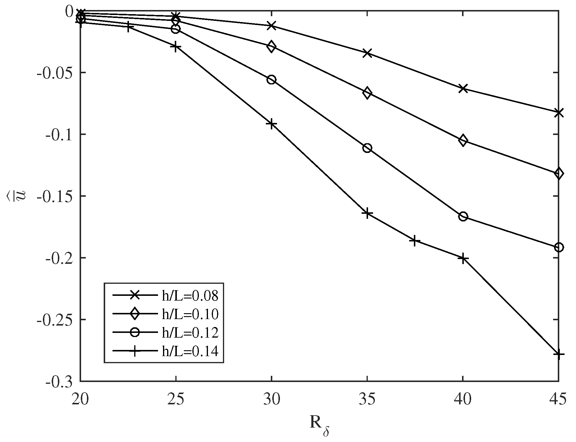The analysis of the steady streaming is carried out by fixing different values of $h/L$ and performing, for each of them, several simulations varying the Reynolds number. Results are shown in Figure 2 for four different values of $h/L$ and $R_{\delta }$ ranging between 20 and 45. In all the cases, it is observed that the steady streaming is negative as it was expected on the basis of the reasoning reported in the previous section. For a fixed value of $h/L$, the steady streaming increases in magnitude when the Reynolds number is increased. The ratio $h/L$ plays a fundamental role in determining the intensity of the steady streaming. Large values of $h/L$ enhance flow separation and the generation of vortices which cause large values of the Reynolds stress $\widehat{\overline{u_1{u}_2}}$. Therefore, the strength of the steady streaming increases with $h/L$ and may attain values comparable with the amplitude of the velocity oscillations. Indeed, for $h/L=0.14$ and $R_{\delta }=45$, $\hat{\overline{u}}\approx 0.28$.

Figure 3 shows the time average of the streamfunction $\psi$ for $R_{\delta }=25$ and $h/L=0.14$ (we remind the reader that the velocity components are given by $u_1=\partial \psi /\partial x_2$, $u_2=-\partial \psi /\partial x_1$). In the figures, red lines denote positive values while black lines denote negative values. In Figure 3a, the parameter r is equal to zero, so that the flow is driven by an oscillating pressure gradient characterized by just one harmonic component, while in Figure 3b the value of r is equal to 0.1 and a second harmonic component is present. Significant differences can be observed between these two cases. When the forcing has just one harmonic component, the time average of streamfunction vanishes far from the bottom (Figure 3a) and the steady streaming consists of two symmetric counter-rotating cells confined close to the bottom. Positive values of the streamfunction characterizes a region of fluid rotating counterclockwise, the opposite for negative values. Therefore, it appears that, close to the bed, the mean flow is directed from the trough towards the crests of the bottom waviness so that, in the presence of a loose bed, the mean flow tends to induce the growth of the ripple amplitude. Figure 3b shows that far from the wall the time average of the streamfunction does not vanish, but it linearly grows with $x_2$ while it is constant along the $x_1$ direction. Therefore, in this case, a steady velocity component in the horizontal direction exists moving far from the bottom which affects the flow in the core region [14,15].

On the top of the negative cell, a saddle point is present and thus the fluid coming from above moves below the negative cell and emerges again before the ripple crest.

Figure 4a shows the spatial distribution of the time-average of the Reynolds stress for $R_{\delta }=25$. It can be observed that large values of the $\overline{u_1{u}_2}$ appear close to the bed, within the recirculating cells. Indeed, the existence of these cells is due to non-vanishing values of the time-average of the Reynolds stress tensor of which $\overline{u_1{u}_2}$ is one of the components. In Figure 4b, the average of $\overline{u_1{u}_2}$ in the $x_1$ direction is shown. Two negative peaks and a positive one can be observed. Overall, negative values of $\widehat{\overline{u_1{u}_2}}$ prevails over positive ones, therefore a negative steady streaming is generated as shown in Figure 3b. Figure 5a shows the spatial distribution of $\overline{u_1{u}_2}$ for $R_{\delta }=40$. In this case, the asymmetric distribution of $\overline{u_1{u}_2}$, due to the presence of a second harmonic component in the pressure gradient that drives the flow is quite evident. The spatial average of $\overline{u_1{u}_2}$ shows a positive peak close to the $x_2$ position where $\overline{u_1{u}_2}$ is maximum. However, in magnitude, the maximum of $\widehat{\overline{u_1{u}_2}}$ occurs at higher elevations, at the edges of the recirculation cells, where $\overline{u_1{u}_2}$ is close to zero ($x_2\approx 10$). Even in this case, overall, negative values of $\widehat{\overline{u_1{u}_2}}$ prevails over positive ones; therefore, a negative steady streaming must be generated.

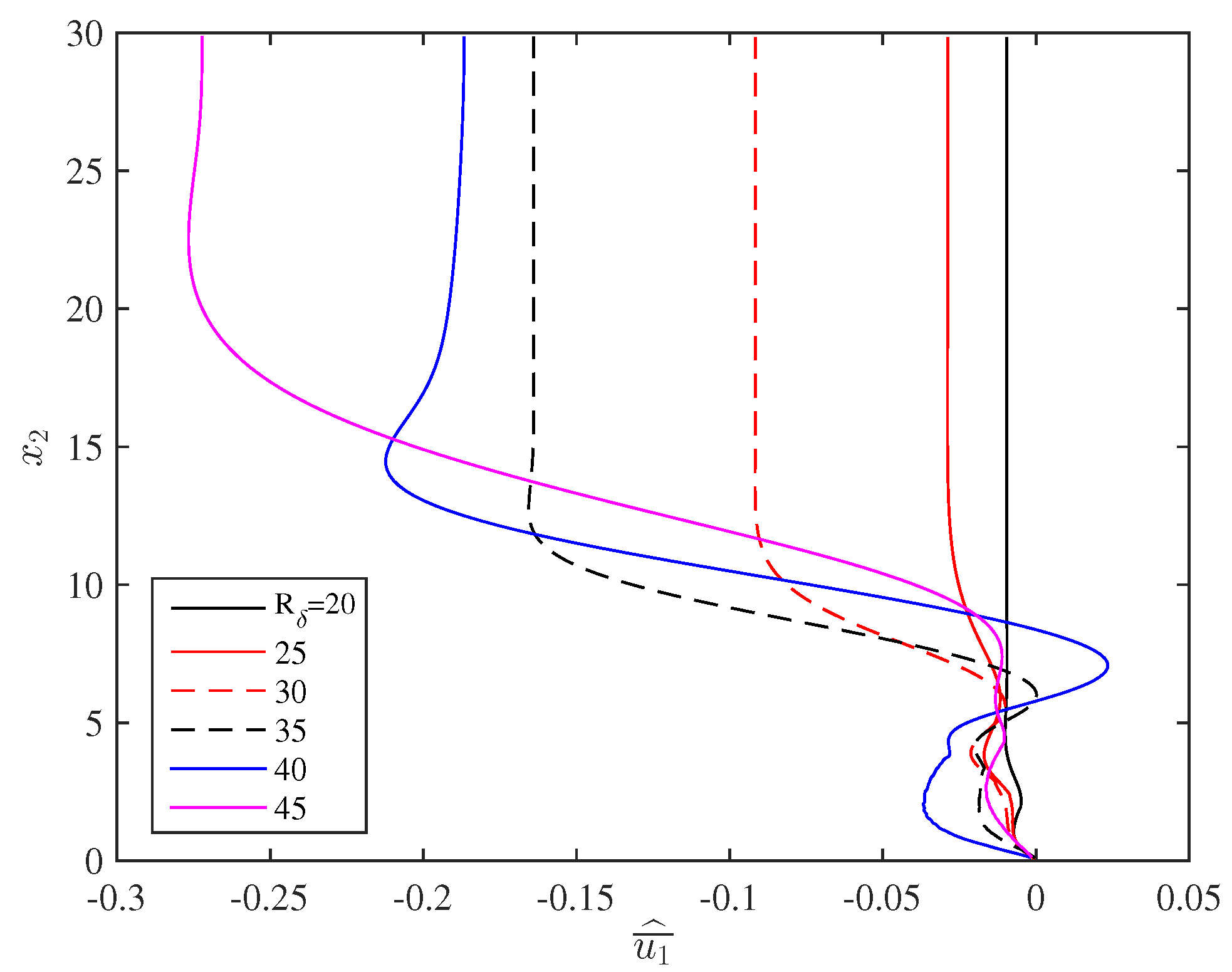
Figure 6 shows the vertical profiles of the steady velocity spatially averaged along the $x_1$ direction ($\widehat{\overline{u_1}}$) for $h/L=0.14$ and $r=0.1$. It can be observed that the strength of the steady streaming increases with the Reynolds number. Near the bed, the velocity is small in a region which extends well above the ripple crest. In this region, positive streaming can also be observed, but it concerns limited areas and this is due to the existence of positive values of $\widehat{\overline{u_1{u}_2}}$ (see Figure 5b). At $x_2\approx 7$, the mean velocity begins to increase rapidly until it attains a constant value where $\widehat{\overline{u_1{u}_2}}$ vanishes (see Equation (12)).

This streaming can be compared with that provided by the formula of [2] reported in the introduction ($0.75U_0^{*2}/c$). However, in doing this, it must be kept in mind that the streaming expressed by this formula is valid for laminar flow on a flat bed and that the mechanism involved is due to the non-uniform velocity distribution in the boundary layer along the longitudinal extension of the surface wave. Instead, the streaming considered in this study is due to the uneven distribution of the Reynolds stress during the flow cycles in the case of a rippled bed. In order to compare these steady streaming with each other, we choose a wave with period of 2 s propagating over a water depth of 2 m. This is a condition that falls within the range of cases considered in experimental studies but is also relevant for field conditions. Using the linear wave theory, we get $c=3.02$ m/s. Assuming a wave height of 0.14 m, we obtain $U_0^{*}=0.056$ m/s. Therefore, according to [2], the streaming is 1.39% of $U_0^{*}$. For this wave, the Reynolds number in the boundary layer turns out to be 44.5; therefore, according to Figure 6, the streaming is approximately 25% of $U_0^{*}$ for $h/L$ = 0.14. This example shows that the streaming due to the mechanism analyzed here can be significantly larger than that due to the mechanism considered by [2].

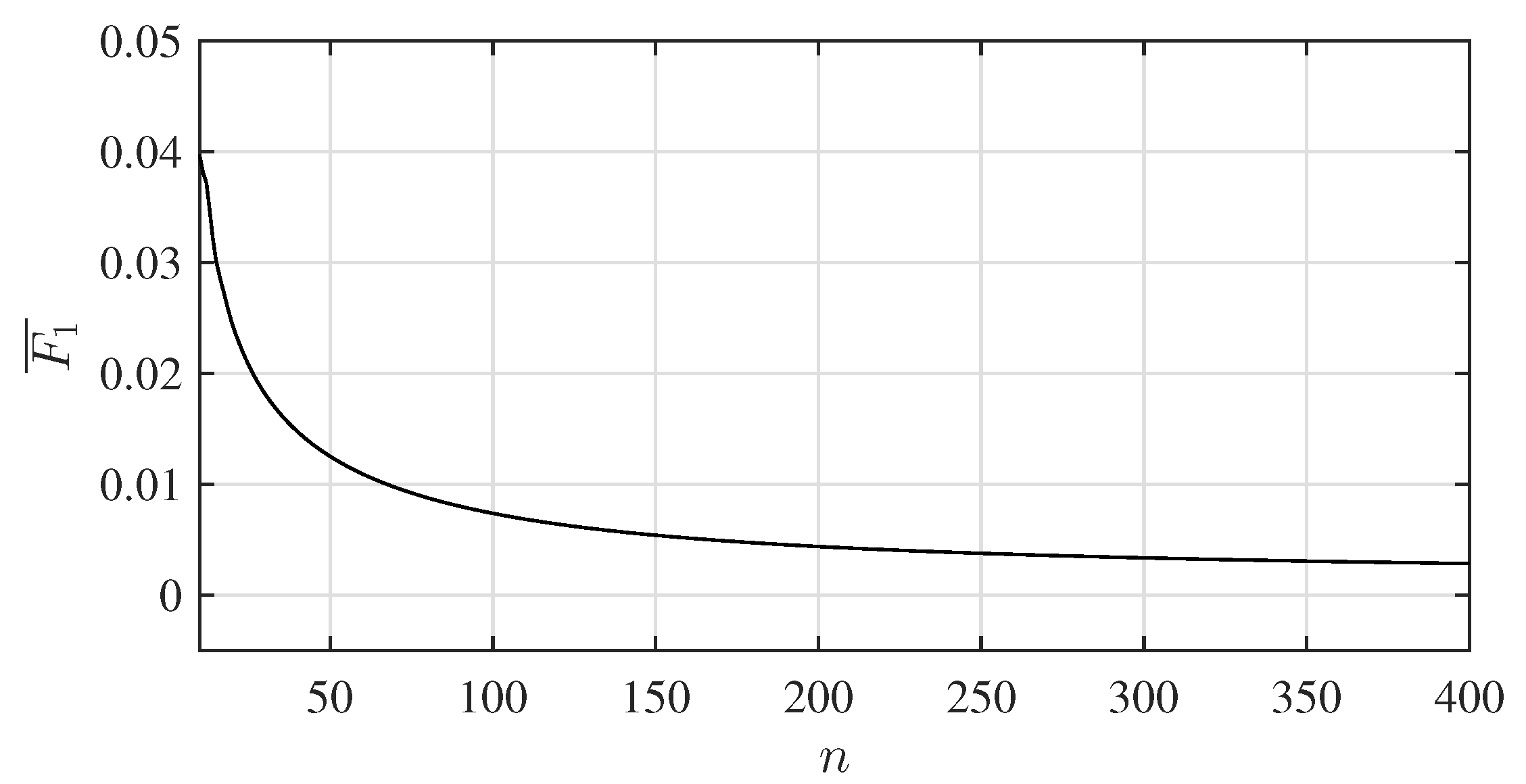
Figure 7 shows the time development of the force acting on a ripple wavelength from the beginning of the numerical simulation. The force attains a steady oscillation after $t=60$, but it clearly appears that the two half cycles are different between themselves because of the asymmetric oscillations. As discussed in Section 3, the time average of the force applied to the bed should vanish when computed on a sufficiently large number of wave cycles. This is shown by Figure 8 where the time average as a function of the number n of wave cycles is reported. It can be noted that, while $F_1$ in Figure 6 is of order 1, its time average rapidly decreases as n increases and attains values smaller than ${10}^{-2}$. This result supports the theoretical finding of Section 3 according to which the time average of $F_1$ vanishes.

5. Conclusions

In the present study, the steady streaming generated over a rippled bed by a purely oscillating pressure gradient is investigated. When the driving pressure gradient is made up of a single harmonic component of angular frequency ${\sigma }^{*}$, the time-averaged velocity field consists of recirculating cells confined near the bed and the time average of both the mean velocity away from the bed and the mean flow rate in the boundary layer vanish. On the other hand, when the driving pressure gradient is the sum of two harmonic components with angular frequency ${\sigma }^{*}$ and $2{\sigma }^{*}$, the mean velocity does not vanish far from the wall and the same occurs for the mean flow rate in the boundary layer. In the latter case, recirculating cells are still present close to the bed although they are not symmetric as it occurs for a sinusoidally oscillating pressure gradient. A more complex flow field would be generated by the interaction of fluid oscillations with the rippled bed when the forcing term has more harmonic components.

The generation of a steady velocity component far from the bed is due to non-vanishing values of the spatial average (in the streamwise direction) of the time-averaged Reynolds stress. When the flow is driven by a sinusoidal oscillating pressure gradient, the time average of the Reynolds stress is symmetrically distributed along the $x_1$ direction as positive and negative values appear equally and the horizontal average vanishes. On the other hand, when the driving pressure gradient is the sum of two harmonic components, the turbulence intensity is not equally distributed during the two half-cycles so that positive and negative values of the time-averaged Reynolds stress do not appear equally in the space. Generally, for asymmetric waves, negative values prevail as turbulence is more intense when the velocity is positive. Therefore, the spatial average of the time-averaged Reynolds stress is negative and this causes a steady streaming even far from the bed.

Although a steady velocity component develops within the boundary layer and the mean flow rate is different from zero, in contrast to steady flows driven by a time constant pressure gradient, the time-average of the force applied to the bed vanishes.

In principle, the present study could easily be extended to include more harmonics in order to consider a random flow. For this purpose, a realistic random series of velocities at the edge of the boundary layer, due to waves characterized by a certain degree of asymmetry, should be determined. Currently, there are no well-established methods for generating such a time series. To this end, however, it would be possible to use the data derived from velocity measurements just outside the boundary layer under random shoaling waves, which have the asymmetry characteristics considered here.