Challenges in Description of Nonlinear Waves Due to Sampling Variability

Abstract

Wave description is affected by several uncertainties, with sampling variability due to limited number of observations being one of them. Ideally, temporal/spatial wave registrations should be as large as possible to eliminate this uncertainty. This is difficult to reach in nature, where stationarity of sea states is an issue, but it can in principle be obtained in laboratory tests and numerical simulations, where initial wave conditions can be kept constant and intrinsic variability can be accounted for by changing random seeds for each run. Using linear, second-order, and third-order unidirectional numerical simulations, we compare temporal and spatial statistics of selected wave parameters and show how sampling variability affects their estimators. The JONSWAP spectrum with gamma peakedness parameters γ = 1, 3.3, and 6 is used in the analysis. The third-order wave data are simulated by a numerical solver based on the higher-order spectral method which includes the leading-order nonlinear dynamical effects. Field data support the analysis. We demonstrate that the nonlinear wave field including dynamical effects is more sensitive to sampling variability than the second-order and linear ones. Furthermore, we show that the mean values of temporal and spatial wave parameters can be equal if the number of simulations is sufficiently large. Consequences for design work are discussed.

1. Introduction

The sea surface is random; therefore, wave parameters derived from a temporal or spatial wave record will depend on which part of a wave record is used in the analysis, as well as on the length of a wave record and/or size of the investigated ocean area (see, e.g., References [1,2,3,4,5,6]). The error introduced by a limited wave record length/domain represents statistical uncertainty, called sampling variability, which can be reduced by increasing duration/ocean area of measurements/numerical simulations. Ideally, temporal/spatial wave registrations should be as large as possible to eliminate sampling variability. This is difficult to reach in nature, where stationarity of sea states is an issue, but it can in principle be obtained in laboratory tests and numerical simulations, where initial wave conditions can be kept constant and intrinsic variability can be accounted for by changing random seeds for each run.

Wave measurements are traditionally recorded at a single point (by buoys, wave probes, lasers, etc.) and restricted to 20 or 30 min, with the duration allowing the assumption of stationarity of a sea state. Spatial wave data are affected by the size of an instrument’s footprint, and they were limited for many years. Recently, their amount increased due to the application of stereo camera systems for collecting space–time ensembles of sea surface elevation, but only a few publications were dedicated to the analysis of these data so far (see, e.g., References [7,8]). Both time and space wave measurements will be affected by sampling variability. This uncertainty brings challenges in the description of ocean waves, particularly nonlinear waves. In the present study, which is an expansion of the investigations carried out by Reference [9], we address this topic, having in mind engineering applications.

Awareness of the presence of sampling variability in wave observations existed for decades, but analysis of its effect on wave characteristics for many years was mostly limited to temporal data (e.g., References [3,10,11,12,13,14]). Focus on the importance of applying spatial statistics in wave description started to increase in the last decade, particularly due to the introduction of the Piterbarg theorem [15] to oceanography in 2004 by Krogstad et al. [16], showing that single-point temporal measurements may greatly underestimate the actual maximum wave displacements that can occur on sea surface areas, especially in short-crested seas. The theorem was verified later in a laboratory setting by Forristall [17,18].

The Piterbarg theorem is based on homogeneous Gaussian fields and the asymptotic extreme value distribution for the maximum of the wave field. It uses Rice’s formula and the Poisson property of high up-crossings, leading to an asymptotic expression for the maximum wave displacement, which is expected to be more accurate as the number of observations increases. The theorem gives no recommendations on how large this number should be. Thus, the results based on the Piterbarg theorem must be viewed as an approximation, which is approximately valid for linear wave fields. The theorem was extended to second order (namely, the Piterbarg–Tayfun distribution) by Socquet-Juglard et al. [19] and used by Reference [7] to study distribution of extreme crest heights in low sea states (significant wave height below 1.5 m), showing satisfactory fit. The Piterbarg–Tayfun distribution was also applied by Reference [20] to investigate the sea state during the Prestige accident. The authors showed that this accident happened in a crossing sea state, with a crossing angle of about 90°, but they were not able to identify any increased probability of rogue waves for this sea state. Later, Gramstad et al. [4] demonstrated, investigating crossing wave systems, that, because of the effects described by Piterbarg for a linear sea state, the expected maximum crest elevation over a given surface area depends on the crossing angle, such that the expected maximum crest elevation is largest when two wave systems propagate with a crossing angle close to 90°. It was further documented by third-order HOSM (higher-order spectral method) simulations that nonlinearities have an opposite effect, such that sea surface kurtosis (identifying occurrence of extreme events in a wave record) has a minimum around 90°, and it is expected to have a maximum for relatively large and small crossing angles.

The investigations addressing area effects on wave characteristics also received attention in the marine industry, which traditionally uses temporal statistics in design. Particularly, focus on the impact of spatial effects on extreme crest heights, being of great importance for engineering applications, increased continuously in the last few years. Theoretical, numerical, and experimental studies were dedicated to this topic; most of them, however, were restricted to short-term statistics and a limited number of sea states (for a review, see, e.g., Reference [21]). Forristall [17,18], based on theory and laboratory data, proposed a procedure for the correction of extreme wave crest due to spatial variability of the sea surface in a sea state. The study of Hagen et al. [21] was the only one that considered the area effects on the long-term statistics of waves. An extensive number of numerical linear and second-order time-domain simulations over the complete scatter diagram of significant wave height and spectral wave period were carried out for a selected location in the northern North Sea. Based on these simulations, the authors expressed the maximum crest height as a function of the jacket’s platform deck dimensions and demonstrated that the spatial effect for the design values is somewhat higher for the second-order sea than for the linear sea. It should also be mentioned that the Norwegian Standard NORSOK [22] recommends a 10% increase in estimated extreme crest height compared to second-order point statistics to account for nonlinear waves and spatial statistics for the finite deck area of offshore structures.

In the present paper, we investigate impact of nonlinearities of a wave field on the wave spatial and temporal statistics in selected sea states characterized by increasing wave steepness. The sea states where rogue waves were recorded in nature are considered, albeit assuming that the wave field is unidirectional. The Pierson–Moskowitz and the JONSWAP spectrum with different gamma parameters were used in the analysis, which included linear, second-order, and third-order theories. The third-order wave data were simulated using the nonlinear HOSM wave model, which included the leading-order nonlinear dynamical effects, accounting for the effect of modulational instability. Wave parameters, characterizing the nonlinearity of sea surface, such as the maximum wave crest, skewness, and kurtosis, were investigated. Examples with directional simulations and field data supported the analysis. The impact of sampling variability on functional relationships between these parameters was demonstrated. Furthermore, it is shown that the nonlinear wave field including dynamical effects is more sensitive to sampling variability than the second-order and linear ones. Consequences of using temporal contra spatial statistics are discussed from the perspective of marine structure design.

2. Set-Up of Numerical Simulations

The investigations carried out were based on simulations with a numerical DNV GL (Det Norske Veritas Germanischer Lloyd) solver based on the higher-order spectral method (HOSM), first proposed by Dommermuth and Yue [23] and West et al. [24]. HOSM has no limitation in terms of the spectral bandwidth of the wave field. Wave fields were simulated in a spatial domain with periodic boundary conditions. The nonlinear order M in the HOSM simulations was set to M = 3 in this study, which included the leading-order nonlinear dynamical effects, including the effect of modulational instability. The solver also included the linear and second-order wave model.

For the unidirectional simulations, the spatial domain was discretized by n_x = 1024 grid points (de-aliased grid), while, in the short-crested simulations, the horizontal plane was discretized using n_x × n_y = 512 × 512 grid points. The domain size in the Fourier space was fixed such that k_x^(max) = k_y^(max) = 8k_p in the fully de-aliased grid (k is the wavenumber and k_p the peak wavenumber). For the unidirectional case, the computational domain corresponded to 64 λ_p, while the directional case corresponded to 32 × 32 λ_p, where λ_p denotes the wavelength corresponding to the peak period T_p. For example, for unidirectional waves with T_p = 10 s on infinite water depth, the computational domain is about 10 km.

The wave fields were simulated in time for a total duration of t_max = 1800 s using a variable-step ODE (ordinary differential equation) solver. A weak dissipation of high wavenumbers was included to model the energy dissipation due to wave breaking, using the dissipation model suggested in Xiao et al. [25]. The breaking option was used only for runs where high wave steepness brought difficulties in the code convergence.

In the simulations, the initial condition was chosen as a wave system with the Pierson–Moskowitz (PM) or the JONSWAP spectrum and with a ${\cos }^N(\varphi -{\varphi }_p)$ directional spreading function for the short-crested simulation, where ϕ is the wave direction and ϕ_p is the peak direction of propagation.

Thus, the wave spectrum was defined as $E(k)=F(k)D(\varphi )$, where k = (k_x,k_y) = $k(\sin \varphi ,\cos \varphi )$, and

$$F(k)=\frac{\alpha }{2k^3}\exp \left[-\frac{5}{4}{\left(k/k_p\right)}^{-2}\right]{\gamma }^{\exp \left[-\frac{{(\sqrt{k/k_p}-1)}^2}{2{\sigma }^2}\right]},$$

(1)

and

$$\begin{array}{cc}D(\varphi )=\frac{1}{k\sqrt{\pi }}\frac{\mathsf{\Gamma }(N/2+1)}{\mathsf{\Gamma }(N/2+1/2)}{\cos }^N(\varphi -{\varphi }_p),& if\left|\varphi -{\varphi }_p\right|\le \frac{\pi }{2}\\ (D(\varphi )=0 \mathrm{otherwise}),\end{array}$$

(2)

where, Γ is the gamma function, and the parameter σ has the standard values 0.07 for k $\le$ k_p and 0.09 for k > k_p. The other spectral parameters α, γ, k_p, ϕ_p, and N were chosen to give the desired spectral shape, significant wave height H_s, and peak period T_p. N denotes the directional spreading coefficient.

The following gamma peakedness parameters were used in the analysis: γ = 1, 3.3, and 6. Note that, for γ = 1, the JONSWAP spectrum reduces to the Pierson–Moskowitz spectrum. Random phases and amplitudes were assigned to the initial spectrum in all cases. Intrinsic wave variability was accounted for by changing random seeds for each run.

Sea states with increasing wave steepness, k_pH_s/2, in which rogue waves occurred in nature (see Reference [26]), were used in simulations, assuming a unidirectional wave field. For completion, two additional sea states with k_pH_s/2 = 0.13, 0.14, were also included. All considered sea states are listed in

Table 1. Analyzed sea states, deep water. UTC—Coordinated Universal Time.

Case	Date and Time	Hmo (m)	Tp (s)	Wave Steepness
1	1 January 1995, 3:20 p.m. UTC	11.2	16.7	0.08
2	5 February 1999, 4:40 a.m. UTC	7.6	13.0	0.09
3	27 December 1998, 6:40 a.m. UTC	10.4	14.6	0.10
4	25 October 1998, 4:00 p.m. UTC	8.8	12.6	0.11
5	1 December 1999, 2:20 a.m. UTC	7.2	11.3	0.11
6	1 January 1995, 11:00 p.m. UTC	5.7	9.8	0.12
7	Numerical simulations	6.5	10.0	0.13
8	Numerical simulations	6.9	10.0	0.14
9	29 January 2000, 6:40 p.m. UTC	12.1	12.2	0.16

. Note that H_s is derived from the zero-spectral moment, commonly denoted as H_mo. The simulations were carried out for deep-water conditions. Directional numerical data developed in Reference [5], using the approach specified above, were also utilized in the study.

For every sea state, the 1800-s unidirectional HOSM simulations were repeated 1000 times to provide satisfactory statistical estimators of selected wave parameters, while, for directional seas, requiring more central processing unit (CPU) time, they were repeated only 20 times.

3. Results

3.1. Analyzed Wave Parameters

The present analysis is limited to investigations of the maximum surface elevation, as well as theskewness and kurtosis of water surface elevation. Note that the maximum surface elevation ɳ_max, both in time and space, represents a wave crest height, an important parameter in design work and in the selection of rogue waves in a wave record. A common definition of a rogue wave, adopted also herein, is to apply the criteria due to Haver [27], i.e., H_max/H_s > 2 and/or C_max/H_s > 1.25, where C_max and H_max denote the maximum crest height and maximum zero-crossing wave height in a wave time series with significant wave height H_s, defined as four times the standard deviation of the sea surface, typically calculated from a 20-min measurement of the surface elevation. Following the crest criterium, we use herein the ratio C_max/H_s when investigating the maximum surface elevation.

The skewness κ₃ and kurtosis κ₄ coefficients are commonly used to test deviation of population from normality (see Reference [28]). For a Gaussian distributed population, the skewness coefficient is equal to zero and the kurtosis coefficient is equal to three. Wave data include a limited number of observations, thus allowing to provide only sample coefficients of maximum surface elevation, skewness, and kurtosis.

For a surface snapshot from the numerical simulations ${\eta }_{i,j}=\eta (x_i,x_j)$, where i = 1, …, n_x and j = 1, …, n_y (here n_x = n_y = 1024 for unidirectional wave field), the sample skewness κ₃ and the kurtosis κ₄ coefficient can be defined as follows:

$${\kappa }_3=\frac{\frac{1}{n_x{n}_y}{\displaystyle \sum _{i=1}^{n_x}}{\displaystyle \sum _{j=1}^{n_y}{({\eta }_{i,j}-\overline{{\eta }_{i,j}})}^3}}{(\frac{1}{n_x{n}_y}{\displaystyle \sum _{i=1}^{n_x}}{\displaystyle \sum _{j=1}^{n_y}{({\eta }_{i,j}-\overline{{\eta }_{i,j}})}^2{)}^{3/2}}},$$

(3)

$${\kappa }_4=\frac{\frac{1}{n_x{n}_y}{\displaystyle \sum _{i=1}^{n_x}}{\displaystyle \sum _{j=1}^{n_y}{({\eta }_{i,j}-\overline{{\eta }_{i,j}})}^4}}{(\frac{1}{n_x{n}_y}{\displaystyle \sum _{i=1}^{n_x}}{\displaystyle \sum _{j=1}^{n_y}{({\eta }_{i,j}-\overline{{\eta }_{i,j}})}^2{)}^2}}.$$

(4)

The mean value of sea surface $\overline{{\eta }_{i,j}}$ is always zero.

The coefficients κ₃ and κ₄, as well as ɳ_max (C_max), were calculated as averages over all random realizations of the same sea state. The 1800-s simulations, repeated for every sea state 1000 times for unidirectional waves and 20 times for directional sea, were sampled every 0.2 s.

The sample skewness and kurtosis coefficients described by Equation (3) and (4), as well as the alternative “unbiased” commonly used estimators for identically distributed independent samples found in the literature (see, e.g., References [29,30]), represent biased estimators of the real populations of κ₃ and κ₄ in cases where the samples are not independent, which is the case for wave surface oscillations. Therefore, for the numerically simulated linear Gaussian surface, the skewness is not equal exactly to zero nor is the kurtosis equal exactly to three [30]. This effect is more pronounced for small simulation domains (see Reference [4]). Due to the relatively large computation area/duration considered in this study, the presented numerical results are little affected by this bias, but we also observe it.

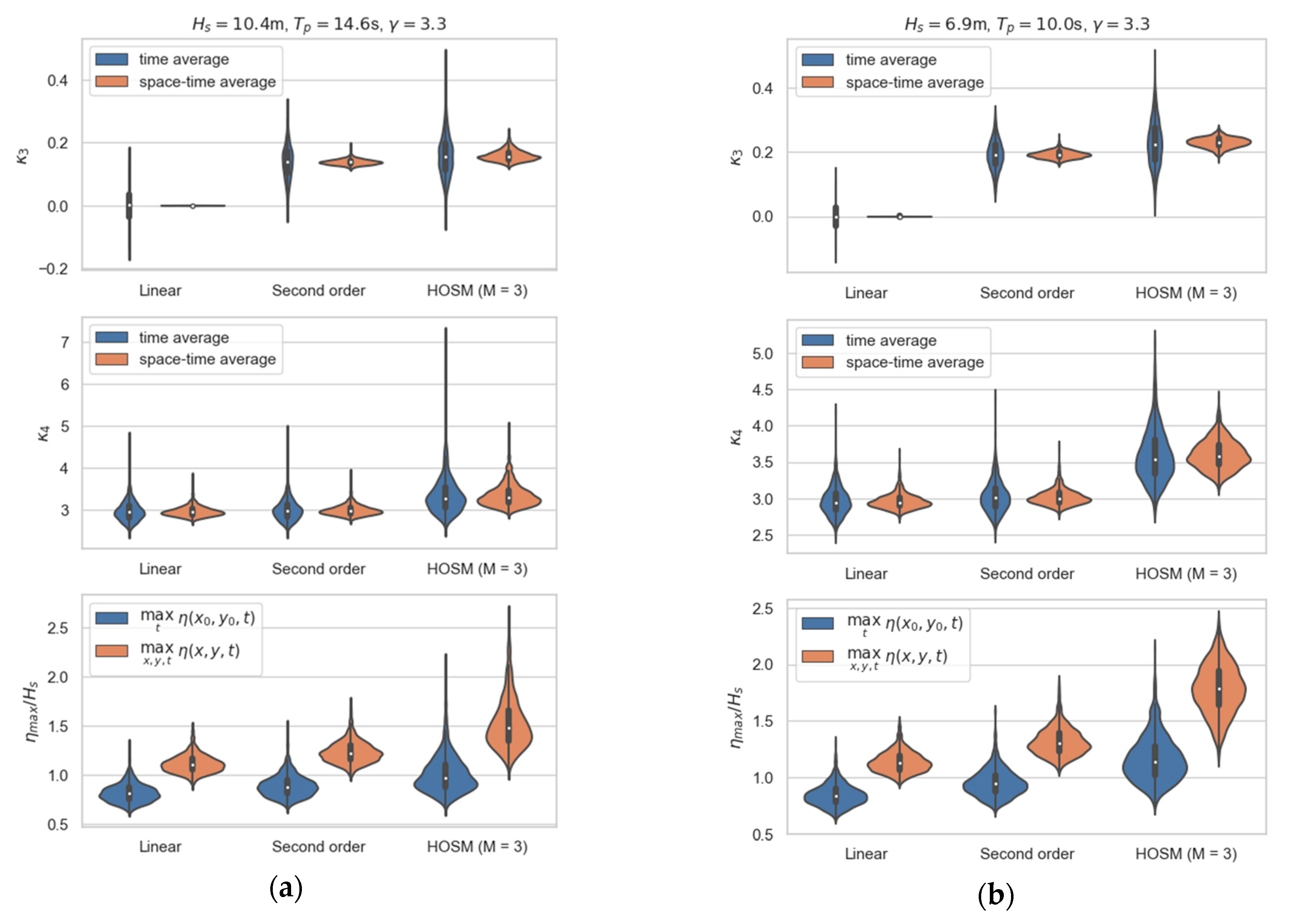
3.2. Comparison of Temporal and Spatial Statistics of Selected Wave Parameters

In Figure 1, Figure 2 and Figure 3, examples of histograms (frequency of occurrence) of temporal (subscript “t”) and spatial (subscript “x,y,t”), from top to bottom, skewness (κ₃), kurtosis (κ₄), and ɳ_max/H_s derived from unidirectional linear, second-order, and HOSM simulations with γ = 1.0 (Figure 1), 3.3 (Figure 2), and 6.0 (Figure 3) are shown. The sea states with the lowest (a) and highest (b) wave steepness, kpH_s/2 = 0.10 and kpH_s/2 = 0.14, are plotted in the figures (see Table 1).

Note that the spatial ɳ_max/H_s, skewness and kurtosis shown in Figure 1, Figure 2 and Figure 3 represent the mean values over the simulation domain averaged over simulation time. The plots in the figures clearly demonstrate the effect of sampling variability manifested by the histograms’ width. The histograms derived from the nonlinear HOSM simulations were much broader than those obtained from the linear and second-order ones, showing that the wave field including nonlinear dynamic effects was more sensitive to sampling variability. Both the wave steepness and the spectral parameter γ impacted the histograms’ width. Furthermore, it is interesting to note also that discrepancies between the estimators obtained from the linear and second-order simulations were not as pronounced as those between the linear and HOSM simulations.

As expected, the spatial ɳ_max/H_s reached higher values compared to the temporal ɳ_max/H_s, for the linear, second-order, and HOSM simulations. The deviations between the linear, second-order, and HOSM-frequency of occurrence functions of ɳ_max/H_s increased with higher γ and wave steepness. This is consistent with earlier findings (e.g. References [31,32]).

The skewness (κ₃) is primarily a second-order effect, while the kurtosis (κ₄) is a third-order effect. Thus, the contribution from nonlinear dynamical effects, including the effect of modulational instability, does not significantly impact the skewness, as also shown in Figure 1, Figure 2 and Figure 3. The mean skewness was around 0.20, as predicted by the second-order wave theory. The coefficient of kurtosis was affected, however, by nonlinear dynamical effects. Although the mean temporal skewness and kurtosis were approximately equal to the mean spatial skewness and kurtosis, the shape of the temporal and spatial histograms and their standard deviations were different. Furthermore, the temporal estimators of skewness and kurtosis reached higher values than the spatial ones for all three wave models, showing that they were more affected by sampling variability than the spatial estimators, as should be expected.

Figure 1, Figure 2 and Figure 3 illustrate the effect pointed out by Reference [6]; for a single simulation, due to sampling variability, ɳ_max/H_s, skewness, and kurtosis derived from linear simulations may reach values close to nonlinear HOSM ones. Furthermore, for a given seed, a single 30-min realization of a sea state may produce a higher kurtosis coefficient for the Pierson–Moskowitz spectrum (JONSWAP spectrum with γ = 1.0) than for the JONSWAP spectrum with γ = 6.0, because of sampling variability.

Figure 4, Figure 5 and Figure 6 show ɳ_max/H_s, skewness, and kurtosis, calculated as the averages over all random realizations of the same sea state, as functions of wave steepness for the linear, second-order, and HOSM simulations with γ = 1.0, 3.3, and 6.0, respectively. Both temporal and spatial estimators derived from unidirectional simulations, together with the 95% confidence intervals, are plotted in the figures. It is interesting to note that, for the linear and second-order wave model, the PM spectrum (γ = 1.0) gave higher time and space values of ɳ_max/H_s, skewness, and kurtosis than the JONSWAP spectrum with γ = 3.3 and 6.0. This was probably due to the bias of the sample estimators in comparison to the true values, as discussed above. The increase in HOSM skewness with wave steepness was not significantly dependent on the spectral parameter γ, as particularly seen for the temporal skewness estimator.

The HOSM mean ɳ_max/H_s and kurtosis increased with the increase in wave steepness up to kpH_s/2 = 0.14 and slightly decreased afterwards. This can be attributed primarily to nonlinear dynamical effects and not to wave breaking; the breaking option was used only for some runs with kpH_s/2 > 0.14 in the HOSM simulations. Wave breaking may occur for this steepness range, as observed earlier in laboratory experiments (e.g., Reference [32]). For kpH_s/2 > 0.14, non-stationary nonlinear dynamical effects limited the growth of ɳ_max and kurtosis. We did not observe this effect for skewness, which was primarily a second-order effect; however, some reduction in growth of the skewness slope gradient for kpH_s/2 > 0.14 was observed.

For HOSM simulations, Figure 4, Figure 5 and Figure 6 clearly demonstrate the effect of spectrum peakedness related to spectral width on the investigated wave parameters. Consistent with the theory, γ = 6.0 gave the highest ɳ_max/H_s, skewness, and kurtosis, followed by γ = 3.3 and γ = 1.0, both for the time and the space–time estimators.

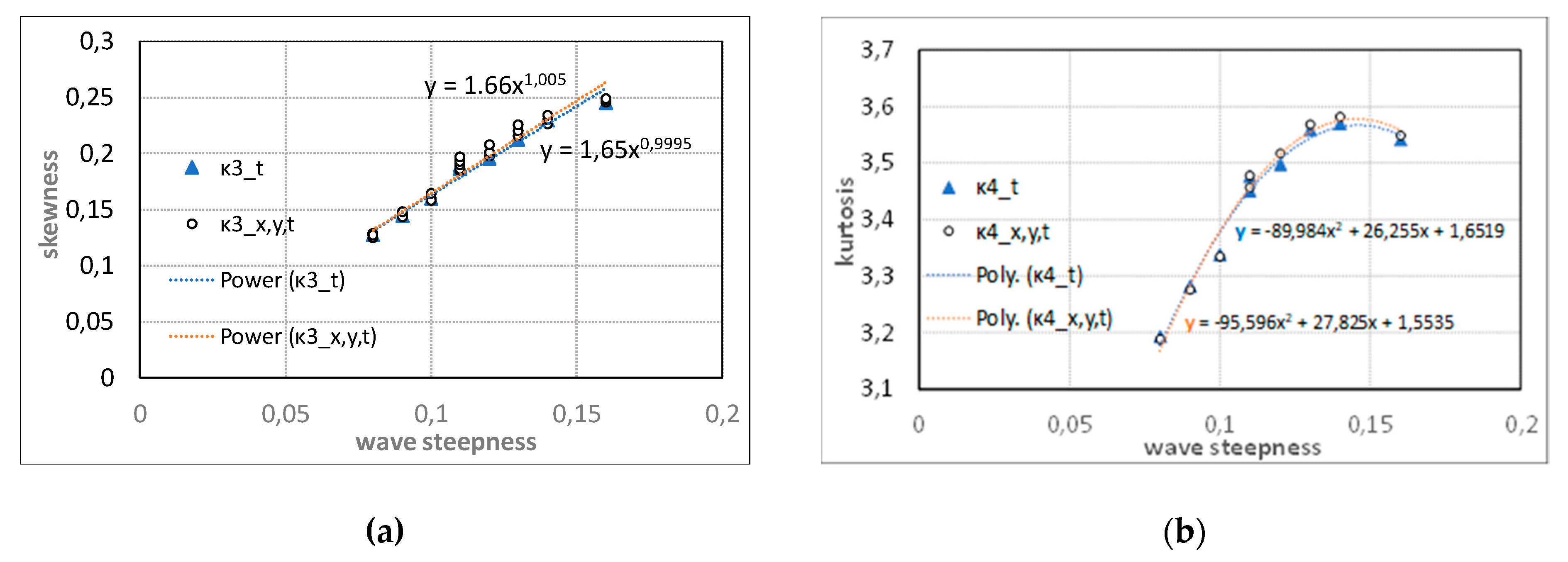
3.3. Correlation between Wave Characteristics and Sampling Variability

Functional relationships between wave characteristics are of importance for design and marine operations. This topic also receives attention in connection with the on-going discussion about the prediction of rogue waves. Commonly, theoretical/semi-theoretical expressions need to be verified through field data. Regarding rogue waves, even though the theory pointed out some parameters as indicators of rogue wave occurrence, wave researchers were unable to get confirmation of the theory in the analysis of measurements. Large clouds of data did not allow drawing any regression lines between wave parameters identifying the occurrence of rogue wave (see, e.g., References [33,34]). For a long time, it was not clear why the issue was so difficult to solve. Today, we know that sampling variability brings these challenges.

To illustrate the problem, Figure 7 shows an example of continuous single-point measurements of significant wave height, kurtosis, and skewness registered on 2 January 2016. The parameters plotted in the figure were calculated from time series of sea surface elevation recorded with a sampling rate of 2 Hz by a WaveRadar REX (known also as SAAB REX radar) at the Ekofisk field in central North Sea. The gray areas around the average values of Hs, kurtosis (Ku in the figure), or skewness in the figures show the standard deviations (representing sampling variability) of the parameters, derived following the procedure proposed by Reference [3], i.e., 20-min parameters (Hs, Ku, skewness) were calculated for all 20-min periods starting at 1-min intervals within each 60 min. The black dots are these values. Large spreading around the measured values can be observed. The 20- and 60-min average values of Hs, skewness, and kurtosis, also plotted in the figure, clearly demonstrate how the increase of the measurement duration reduced the sampling variability. Note that the 20-min average values are marked by the dark-blue color while the 60-min values are marked by the red color.

The effect of sampling variability on field data is also demonstrated in Figure 8, where standard deviations of skewness and kurtosis, as described for Figure 7, derived from 20-min wave records, registered continuously at a single point by the WaveRadar REX, are plotted against the 1-h average skewness and kurtosis values. The data cover the period from January 2016 to September 2019. The standard deviations of these parameters were derived following the procedure proposed by Reference [3]. The mean and median are also plotted in the figure. As expected, large spreading, due to sampling variability, can be observed. It is interesting to see consistency with the numerical simulations; temporal skewness was much more affected by sampling variability than temporal kurtosis. While the mean standard deviation of kurtosis increased with the increase in kurtosis, we did not observe this for skewness, but instead saw a cloud of data. Furthermore, as expected, the unidirectional simulations shown in Figure 4, Figure 5 and Figure 6 had larger spreading than the field data presented in Figure 8.

Below, we show how numerical simulations can help to reduce deviations between temporal and spatial statistics and allow establishing a correlation between the wave parameters responsible for occurrence of rogue waves.

In Figure 9, the averages of temporal and spatial skewness and kurtosis, over all unidirectional random realizations of the same sea state with γ = 3.3, are plotted as a function of wave steepness. As expected, the average temporal and spatial estimators of skewness and kurtosis were approximately equal, due to the large numbers of runs carried out.

For unidirectional wave fields, the mean temporal/spatial skewness is not sensitive to the spectral parameter γ, and a general expression independent of γ, as shown in Figure 9a for γ = 3.3, can be proposed for skewness as a function of wave steepness.

κ_{3_x,y,t} = 1.66(k_pH_s/2).

(5)

This formula can be compared to the expression suggested by Reference [35].

Although the average temporal and space–time estimators of HOSM skewness and kurtosis over all runs were approximately equal, there was significant spreading around the mean values, which was larger for the temporal data than for the spatial data. The coefficient of variation (COV) was up to 0.53 for the temporal skewness and up to 0.12 for the spatial one (the time dataset was smaller than the spatial one), while, for kurtosis, COV was up to 0.16 for temporal data and up to 0.11 for spatial data.

In Figure 10a, the mean spatial kurtosis over all runs as a function of wave steepness for γ = 1.0, 3.3, and 6.0 is shown, together with the fitted to the data polynomials. The figure confirms that when the mean values over a large number of runs are considered, it is not difficult to establish a correlation between wave parameters, which is consistent with wave theory. Furthermore, it should be noted that the results presented herein refer to unidirectional wave fields, giving more conservative estimators than we would expect when analyzing directionally spread waves. To document this, for comparison, Figure 10a includes the kurtosis calculated from the directional HOSM simulations of Reference [6] for k_pH_s/2 = 0.11, with γ = 1.0 and N = 4 (N is the spread number), with γ = 3.3 and N = 16, and with γ = 6.0 and N = 100. As expected, the effect of modulational instability was suppressed when the wave energy spreading was accounted for.

Although small deviations between the mean over all runs of skewness and kurtosis were identified, the picture was different for the average temporal and spatial ratio of the maximum surface elevation divided by significant wave height, ɳ_max/H_s. The average ɳ_max/H_s over all runs as a function of wave steepness is shown together with the fitted polynomials in Figure 10b. The spatial ɳ_max/H_s differed significantly from the temporal one, largely exceeding the temporal values. Furthermore, the shape of the wave spectrum affected the spatial ɳ_max/H_s more than the temporal one. The observed deviations between temporal and spatial estimators were due to the limited data. Increasing the number of simulations should reduce these deviations.

The results shown in Figure 10b demonstrate the importance of considering area effects on the maximum wave crest height when designing marine installations.

4. Discussion and Conclusions

The inherent variability of sea surface elevation brings challenges in the description of ocean waves because of sampling variability, i.e., the statistical uncertainty due to a limited number of observations. For limited wave records, whether over duration or over ocean area, depending on which part of a wave record is taken in an analysis, different estimators of wave parameters are obtained. It should be noted that 20–30-min observations/simulations at a single point will contain less data than space–time measurements/simulations over a restricted ocean area in the same period (given that the sampling rates of the measurements are the same). Thus, wave characteristics obtained from space–time data will always be less affected by sampling variability than those derived from time series. However, more important than the number of observations (which depends on the sampling rate of the measurements) are the dimensions of the selected ocean area relative to the dimensions of the measured waves (i.e., the typical wavelength and period). Increasing a sampling step alone will increase the number of data points, but not the accuracy of the estimators of wave characteristics derived from them.

The results presented in the paper are based primarily on numerical unidirectional HOSM simulations, and they are supported by examples with directional HOSM simulations and field data. The HOSM simulations are restricted to the third-order of nonlinearity which includes the leading-order nonlinear dynamical effects, including the effect of modulational instability. From the earlier investigations, we do not expect that increasing the order of nonlinearity in HOSM will change the present conclusions. Furthermore, the domain size in the Fourier space was fixed in the analysis such that k_x^(max) = k_y^(max) = 8k_p in the fully de-aliased grid. This means that changing the number of grid points affected the size of the domain in x/y-space, as well as the grid-spacing in wavenumber space. In order to obtain “converged” results, it is important to have a sufficiently large physical domain, as well as sufficiently fine resolution of the wavenumber space. Hence, a larger number of grid points is generally an advantage. Based on our own experience with HOSM, as well as from numerous studies using HOSM in the scientific literature, we can say that our choice of discretization is sufficient to obtain “converged” results with respect to discretization. Although we previously carried out convergence studies, we did not do this specifically for the current paper.

Herein, we compared the temporal and spatial statistics of selected wave parameters derived from unidirectional numerical linear, second-order, and HOSM simulations for the JONSWAP gamma peakedness parameter γ = 1, 3.3, and 6. The maximum surface elevation, skewness, and kurtosis were considered. It is shown that the nonlinear wave field including dynamical effects is more sensitive to sampling variability than the second order and linear ones. The dynamical effects have a significant impact on the analyzed parameters, particularly on ɳ_max/H_s. The discrepancies between the wave parameter estimators derived from the HOSM simulations and the linear ones are much larger than those obtained from the second-order and linear simulations. We show that the mean values of temporal and spatial wave parameters can be equal if the number of simulations is sufficiently large. Furthermore, we proposed functional relationships between the investigated parameters and wave steepness.

When using a single 20- or 30-min field wave record, it is challenging to conclude the importance of nonlinearity of surface elevation, since the sampling variability may dominate over the nonlinear effects. Therefore, numerical models and laboratory tests represent important supporting tools to field data in this respect. They also allow establishing functional relationships between wave parameters, which are often not possible to derive from field data, if the number of observations is not sufficiently large. We should, however, be aware of that variability is also related to such expressions.

The results presented were developed using extensive computations with relatively large domain/duration. A reduction of the area would increase the spreading around the calculated estimators of wave parameters. Furthermore, the results of this study were derived for unidirectional wave fields; therefore, they should be applied with care in engineering applications, as they represent conservative estimators of wave parameters. The examples of the directional HOSM simulations presented in the paper confirm this.

New installations of stereo video camera systems, e.g., the Norwegian Meteorological Institute stereo video camera system based on the method developed at ISMAR (Institute of Marine Sciences, Venice, Italy) by [7], will allow obtaining further insight into temporal and space–time statistics and the associated sampling variability.

Knowledge about uncertainty due to sampling variability is essential for design work and marine operations.

References

1. Bitner-Gregersen, E.M.; Hagen, Ø. Uncertainties in Data for the Offshore Environment. Struct. Saf. 1990, 7, 11–34. [Google Scholar] [CrossRef]
2. Bitner-Gregersen, E.M. Sea state duration and probability of occurrence of a freak wave. In Proceedings of the OMAE 2003, Cancun, Mexico, 8–13 June 2003. [Google Scholar]
3. Bitner-Gregersen, E.M.; Magnusson, A.K. Effect of intrinsic and sampling variability on wave parameters and wave statistics. Ocean Dyn. 2014, 64, 1643–1655. [Google Scholar] [CrossRef]
4. Gramstad, O.; Bitner-Gregersen, E.M.; Trulsen, K.; Nieto Borge, J.C. Modulational instability and rogue waves in crossing sea states. J. Phys. Oceanogr. 2018, 48, 1317–1331. [Google Scholar] [CrossRef]
5. Gemmrich, J.; Thomson, J.; Erick Rogers, W.; Pleskachevsky, A.; Lehner, S. Spatial characteristics of ocean surface waves. Ocean Dyn. 2016, 66, 1025–1035. [Google Scholar] [CrossRef]
6. Bitner-Gregersen, E.M.; Gramstad, O. Impact of sampling variability on sea surface characteristics of nonlinear waves. In Proceedings of the OMAE 2018 Conference, Madrid, Spain, 17–22 June 2018. [Google Scholar]
7. Benetazzo, A.; Barrariol, F.; Bergamasco, F.; Torsello, A.; Carniel, S.; Sclavo, M. Observation of Extreme Sea Waves in a Space–Time Ensemble. Am. Meteorol. Soc. 2015, 45, 2261–2275. [Google Scholar] [CrossRef] [Green Version]
8. Benetazzo, A.; Barrariol, F.; Bergamasco, F.; Torsello, A.; Carniel, S.; Sclavo, M. On the shape and likelihood of oceanic rogue waves. Sci. Rep. 2017, 7, 8276. [Google Scholar] [CrossRef]
9. Bitner-Gregersen, E.M.; Gramstad, O. Comparison of temporal and spatial statistics of nonlinear waves. In Proceedings of the OMAE 2018 Conference, Glasgow, UK, 9–14 June 2019. [Google Scholar]
10. Longuet-Higgins, M.S. On the statistical distribution of the heights of sea waves. J. Mar. Res. 1952, 11, 245–266. [Google Scholar]
11. Donelan, M.A.; Pierson, W.J. The sampling variability of estimates of spectra of wind generated gravity waves. J. Geophys. Res. 1983, 88, 4381–4392. [Google Scholar] [CrossRef]
12. Young, I.R. Probability distribution of spectral integrals. J. Waterw. Ports Coast. Ocean Eng. 1986, 112, 338–341. [Google Scholar] [CrossRef]
13. Forristall, G.Z.; Heideman, J.C.; Leggett, I.M.; Roskam, B.; Vanderschuren, L. Effect of sampling variability on hindcast and measured wave heights. J. Waterw. Port Coast. Ocean Eng. 1996, 122, 216–225. [Google Scholar] [CrossRef]
14. Tucker, M.J. Recommended Standard for Wave Data Sampling and Real Time Processing; Tech. Rep.3, 14/186; E&P Forum: London, UK, 1992; pp. 25–28. [Google Scholar]
15. Piterbarg, V.I. Asymptotic methods in the theory of Gaussian processes and fields. AMS Transl. Math. Monogr. 1996, 148. [Google Scholar]
16. Krogstad, H.E.; Liu, J.; Socquet-Juglard, H.; Dysthe, K.B.; Trulsen, K. Spatial extreme value analysis of nonlinear simulations of random surface waves. In Proceedings of the OMAE 2004, OMAE 51336, Vancouver, BC, Canada, 20–25 June 2004. [Google Scholar]
17. Forristall, G. Maximum Crest Heights under a Model TLP Deck. In Proceedings of the 30th International Conference on Offshore Mechanics and Arctic Engineering, OMAE2011-49837, Rotterdam, The Netherlands, 19–24 June 2011. [Google Scholar]
18. Forristall, G. Maximum Crest Heights over an Area: Laboratory Measurements Compared to Theory. In Proceedings of the 34th International Conference on Ocean, Offshore and Artic Engineering, OMAE2015-41061, St. John’s, NL, Canada, 31 May–5 June 2015. [Google Scholar]
19. Socquet-Juglard, H.; Dysthe, K.; Trulsen, K.; Krogstad, H.E.; Liu, J. Probability distributions of surface gravity waves during spectral changes. J. Fluid Mech. 2005, 542, 195–216. [Google Scholar] [CrossRef] [Green Version]
20. Trulsen, K.; Nieto Borge, J.C.; Gramstad, O.; Aouf, L.; Lefèvre, J.M. Crossing sea state and rogue wave probability during the Prestige accident. J. Geophys. Res. Oceans 2015, 120, 7113–7136. [Google Scholar] [CrossRef] [Green Version]
21. Hagen, Ø.; Birknes-Berg, J.; Grue, I.H.; Lian, G.; Bruserud, K.; Vestbøstad, T. Long-term area statistics for maximum crest height under fixed platform deck. In Proceedings of the OMAE 2018 Conference, OMAE2019-77263, Madrid, Spain, 17–22 June 2018. [Google Scholar]
22. NORSOK. The Norwegian Standard N-003, Edition 3, Action and Action Effects; NORSOK: Oslo, Norway, January 2017. [Google Scholar]
23. Dommermuth, D.G.; Yue, D.K. A high–order spectral method for the study of nonlinear gravity waves. J. Fluid Mech. 1989, 184, 267–288. [Google Scholar] [CrossRef]
24. West, B.J.; Brueckner, K.A.; Jand, R.S.; Milder, D.M.; Milton, R.L. A new method for surface hydrodynamics. J. Geophys. Res. 1987, 92, 11803–11824. [Google Scholar] [CrossRef]
25. Xiao, W.; Liu, Y.; Wu, G.; Yue, D.K.P. Rogue wave occurrence and dynamics by direct simulations of nonlinear wave-field evolution. J. Fluid Mech. 2013, 720, 357–392. [Google Scholar] [CrossRef]
26. Bitner-Gregersen, E.M.; Magnusson, A.K. Extreme Wave Events in Field Data and in a Second Order Wave Model. In Proceedings of the ROGUE’2004 Conference, Brest, France, 20–22 October 2004. [Google Scholar]
27. Haver, S. Evidences of the Existence of Freak Waves. In Proceedings of the ROGUE Waves 2000, Brest, France, 29–30 November 2000; pp. 129–140. [Google Scholar]
28. Longuet-Higgins, M. The effect of non-linearities on statistical distributions in the theory of sea waves. J. Fluid Mech. 1963, 17, 459–480. [Google Scholar] [CrossRef]
29. Bai, J.; Ng, S. Tests for Skewness, Kurtosis, and Normality for Time Series Data. J. Bus. Econ. Stat. 2005, 23, 49–60. [Google Scholar] [CrossRef] [Green Version]
30. Bao, Y. On sample skewness and kurtosis. Econom. Rev. 2013, 32, 415–448. [Google Scholar] [CrossRef]
31. Onorato, M.; Osborne, A.; Serio, M.; Cavaleri, L.; Brandini, C.; Stansberg, C. Extreme waves, modulational instability and second order theory: Wave flume experiments on irregular waves. Eur. J. Mech. B Fluids 2006, 25, 586–601. [Google Scholar] [CrossRef]
32. Toffoli, A.; Gramstad, O.; Trulsen, K.; Monbaliu, J.; Bitner-Gregersen, E.M.; Onorato, M. Evolution of weakly nonlinear random directional waves: Laboratory experiments and numerical simulations. J Fluid Mech. 2010, 664, 313–336. [Google Scholar] [CrossRef]
33. Olagnon, M.; Magnusson, A.K. Sensitivity study of sea state parameters in correlation to extreme wave occurrences. In Proceedings of the 14th International Offshore and Polar Engineering Conference, ISOPE 3, Toulon, France, 23–28 May 2004. [Google Scholar]
34. Olagnon, M.; Magnusson, A.K. Spectral parameters to characterize the risk of rogue wave occurrence in a sea state. In Proceedings of the ROGUES’2004 Conference, Brest, France, 20–22 October 2004. [Google Scholar]
35. Vinje, T.; Haver, S. On the non-Gaussian structure of ocean waves. In Proceedings of the BOSS’94 Conference, Cambridge, MA, USA, 12–15 July 1994; Volume 2, pp. 453–480. [Google Scholar]
Figure 1. Temporal (blue) and space–time (brown) histograms of skewness, kurtosis, and ɳmax/Hs for unidirectional linear, second-order, and HOSM (higher-order spectral method) simulations for sea states (a) kpHs/2 = 0.10, γ = 1.0 (left column), and (b) kpHs/2 = 0.14, γ = 1.0 (right column).
Jmse 08 00279 g001
Figure 2. Temporal (blue) and space–time (brown) histograms of skewness, kurtosis, and ɳmax/Hs for unidirectional linear, second-order, and HOSM (higher-order spectral method) simulations for sea states (a) kpHs/2 = 0.10, γ = 3.3 (left column), and (b) kpHs/2 = 0.14, γ = 3.3 (right column).
Jmse 08 00279 g002
Figure 3. Temporal (blue) and space–time (brown) histograms of skewness, kurtosis, and ɳmax/Hs for unidirectional linear, second-order, and HOSM (higher-order spectral method) simulations for sea states (a) kpHs/2 = 0.10, γ = 6.0 (left column), and (b) kpHs/2 = 0.14, γ = 6.0 (right column).
Jmse 08 00279 g003
Figure 4. Estimators of ɳmax/Hs as a function of the wave steepness kpHs/2. Linear (top panel), second-order (center panel), and HOSM (bottom panel) simulations for γ = 1.0 (blue), 3.3 (green), and 6.0 (brown). The bars represent the 95% confidence interval. (a) Temporal simulations; (b) spatial simulations.
Jmse 08 00279 g004
Figure 5. Estimators of skewness as a function of the wave steepness kpHs/2. Linear (top panel), second-order (center panel), and HOSM (bottom panel) simulations for γ = 1.0 (blue), 3.3 (green), and 6.0 (brown). The bars represent the 95% confidence interval. (a) Temporal simulations; (b) spatial simulations.
Jmse 08 00279 g005
Figure 6. Estimators of kurtosis as a function of the wave steepness kpHs/2. Linear (top panel), second-order (center panel), and HOSM (bottom panel) simulations for γ = 1.0 (blue), 3.3 (green), and 6.0 ( brown). The bars represent the 95% confidence interval. (a) Temporal simulations; (b) spatial simulations.
Jmse 08 00279 g006
Figure 7. Continuous records of significant wave height (upper panel), kurtosis (middle panel), and skewness (lower panel). Measurements were registered using the WaveRadar REX at Ekofisk field in central North Sea on 2 January 2016.
Jmse 08 00279 g007
Figure 8. Standard deviations of temporal skewness (a) and kurtosis (b) derived from 20-min continuous measurements registered using the WaveRadar REX at the Ekofisk field. The data are plotted against the 1-h average values of skewness and kurtosis.
Jmse 08 00279 g008
Figure 9. Average over all runs of temporal and spatial (a) skewness versus wave steepness; (b) kurtosis versus wave steepness. HOSM simulations, γ = 3.3.
Jmse 08 00279 g009
Figure 10. Average over all runs of spatial (a) kurtosis versus wave steepness, and (b) ɳmax/Hs versus wave steepness. HOSM simulations, γ = 1.0 (black line), 3.3 (blue line), and 6.0 (brown line). Panel (a) also includes the spatial kurtosis for directional waves: γ = 1.0 with spread number N = 4 (black mark), γ = 3.3 with N = 16 (blue mark), and γ = 6.0 with N = 100 (brown mark), while Panel (b) includes the temporal ɳmax/Hs versus wave steepness, where red, violet, and gray lines (the three lower lines) correspond to γ = 1.0, 3.3, and 6.0, respectively.
Jmse 08 00279 g010