Uncertainties of Estimating Extreme Significant Wave Height for Engineering Applications Depending on the Approach and Fitting Technique—Adriatic Sea Case Study

Abstract

Studies on the extrapolation of extreme significant wave height, based on long-term databases, are extensively covered in literature. An engineer, working in the field of naval architecture, marine engineering, or maritime operation planning, when tackling the problem of extreme wave prediction, would typically follow relevant codes and standards. Currently, authorities in the field of offshore operation within its guidelines propose several methods: the initial-distribution, extreme value, and peak-over threshold approaches. Furthermore, for each proposed method, different mathematical fitting techniques are applicable to optimize the candidate distribution parameters: the least-square method, the method of moments, and the maximum likelihood method. A comprehensive analysis was done to determine the difference in the results depending on the choice of method and fitting technique. All combinations were tested on a long-term database for a location in the Adriatic Sea. The variability of the results and trends of extreme wave height estimates for long return periods are presented, and the limitations of certain methods and techniques are noted.

1. Introduction

Wave statistics are typically considered on a short-term or long-term scale. Long-term statistics, considered in this paper, are typically obtained based on gathered observation data that are collected during a long period of time or based on data from numerical wave model hindcasts. For engineering purposes, e.g., fatigue or mooring analysis, the needed met-ocean data can be directly extracted from histograms of recorded data. Extreme values, on the other hand, usually fall outside the time range of available databases and have to be extrapolated. The accurate prediction of these extremes is indispensable for the risk-based design and operation of ships and offshore structures [1]. Bitner-Gregersen et al. [2] provided an overview of state-of-the-art in sea state analysis by covering topics from wave data acquisition and wave modelling to the application of results in terms of loading input for ships and offshore structural design. When considering wave loading, it is important to keep track of the associated uncertainties. The importance of uncertainties for the matter is recognized by the two most relevant research organization related to ships and offshore structures, namely International Ship and Offshore Structure Congress (ISSC) and International Towing Tank Conference (ITTC). They established a specialists’ committee focused on different types of uncertainties. Related research resulted in series of USMOS (Uncertainty Modelling for Ships and Offshore Structures) workshops [2].

The prediction of extreme significant wave height at a location of interest and for a return period larger than the scope of the available data is done by fitting a theoretical cumulative distribution function F(x) through the available data points and then extrapolating it to the desired probability of occurrence. The cumulative form F(x) of the distribution function is typically used because it is easily linearized by an appropriate scale and plotted as a straight line that facilitates visual fit evaluation.

There is no unique standard approach prescribed in a state-of-the-art scientific analysis or in engineering for long-term, extreme significant wave heights prediction [3,4,5]. Suggested approaches differ in which data they employ, which theoretical distribution is fitted, and which mathematical technique is applied to optimize the fit parameters. Guedes Soares and Henriques [6] reviewed and compared three different fitting techniques for a three-parameter-Weibull distribution on the same dataset. Guedes Soares and Scotto [7] provided a comprehensive literature overview of the uncertainties concerning wave statistics and performed a case study that applied the annual maximum and the peak-over-threshold approaches. Ferreira and Guedes Soares [8] modelled the significant wave height distribution with gamma and beta models, and they covered different distribution tail types for the extreme value theory. Vanem [9] explored uncertainties arising from the distribution choice, the same three methods covered in this paper, on a case study for a location in the North Atlantic for one historical and two future scenarios. The underlying data he used were the results from the WAM wave model, and conclusions were directed at climate change implications. Uncertainty analyses of extreme significant wave height estimations were also done in case studies for the Barents Sea [10], the Norwegian continental shelf, and offshore Alaska [11]. Alternative fitting techniques, such as the genetic optimization algorithm, were tested for estimations of extreme sea states (e.g., [12]).

This study employed three different approaches and three mathematical parameter fitting techniques in parallel. The approaches were the initial distribution (ID) approach with the three-parameter Weibull distribution, the annual maximum (AM) approach with the Gumbel distribution, and the peak-over threshold (POT) approach with the exponential distribution. The three-parameter Weibull distribution (ID approach) is an assumed empirical model while the Gumbel and exponential distributions (used in the AM and POT approaches, respectively) have theoretical justification in extreme value theory (EVT). The Gumbel distribution (AM approach) is a special case of the extreme value distribution (EVD) if the distribution of extremes has an exponential tail. Similarly, the exponential distribution (POT approach) is a special case of the generalized Pareto distribution (GPD). Therefore, the AM and POT methods, as employed in the paper, become compatible with each other within the EVT framework, and, thus, comparisons are significant. Each approach assumes a different preparation of the underlying data, and the underlying Oceanor WorldWaves 23-year database used for the case study is abundant for all three approaches. The mathematical fitting techniques tested for each approach were as follows: the least squares method (LSM), the method of moments (MoM), and the maximum likelihood estimator (MLE). The approaches and fitting techniques were chosen according to current Det Norske Veritas–Germanischer Lloyd (DNV–GL) classification society guidelines applied by engineers when designing structures that require wave loading and statistics as load inputs. DNV–GL is one of the top engineering authorities for offshore structure design. A combination of three approaches and three fitting techniques yielded eight different fits (not nine, since the MoM and MLE fitting techniques produced identical results for the POT approach). Each fit estimated different extreme significant wave height for a 50- and 100-year return period, thus giving a sense of uncertainties corresponding to approach and fitting technique choice.

The aimed contribution of this paper was to provide a comprehensive systematic analysis of different “recommend practice” approaches and fitting techniques proposed by a relevant engineering authority. The difference in the results represented a loss of accuracy due to the arbitrary choice of the approach and the fitting technique applied. These uncertainties are discussed, and their mutual trends are determined depending on the return period. A theoretical extreme for a 23-year return period was also calculated as a verification value, as it fell within the scope of the database and could thus be directly compared.

In the following chapters, the theoretical overview and the governing equations are given, followed by the results and the discussion. Section 2 explains how estimation of the probability of non-exceedance is assigned to empirical datasets. Main features and governing equations are listed for the ID, AM, and POT approaches. Relevant expressions are given for the evaluation of significant wave heights for long return periods based on the fitted theoretical candidate distribution. In Section 3, relevant datasets are extracted from the underlying database and presented in line with the theoretical definition of each approach. For each approach, theoretical distribution fit parameters are reported, and a goodness-of-fit evaluation is presented. In Section 3.4, estimations of significant wave heights are calculated for 50- and 100-year return periods for each theoretical fit. The difference in results is commented upon and uncertainty trends are estimated in Section 4.

2. Methodology

The present study was based on a 23-year database provided by Fugro Oceanor—WorldWaves atlas. The database was originally obtained as a numerical hindcast performed by the third-generation wave model WAM by ECMWF (European Centre for Medium-Range Weather Forecast) and calibrated with satellite altimetry measurements collected from eight different satellite missions: Geosat (1986–1989), Topex (1992–2002), Topex/Poseidon (2002–2005), Jason (2002–2008), EnviSat (2002–2010), Geosat Follow-On (2000–2008), Jason-2 (2008–on-going), and Jason-1s (2009–2012) [13,14]. The database represents a state-of-the-art [2], comprehensive, and systematic (in space and time) source of wave data for the offshore Adriatic Sea basin, as it reports twelve different wave and wind physical parameters in 6 h intervals at 39 locations (Figure 1). Numerically modelled wave data and collected altimetry data joined in a combined dataset were reported with a spatial resolution of 0.5° × 0.5° lat./long., starting from September 1992 to January 2016. The chosen location for the comparative analysis: lat./long. coordinates 13.5° E–45.0° N are located close to Croatian gas fields in the north of the Adriatic Sea. Different methods and fitting techniques were applied for estimating the most probable extreme significant wave heights (H_s) for 50-year and 100-year return periods.

Different approaches (ID, AM, and POT) implied different data preparation methods. Thus, as a first step, the appropriate significant wave height H_s data were extracted from the underlying database. The ID approach used all H_s data points, although a lower cut-off threshold can sometimes be introduced [5]. The AM approach implied that only the yearly H_s maximums were to be used for the analysis. Finally, the POT method meant that the analysis was based on the maximum values (peaks) of storm events that are mathematically defined as an uninterrupted number of H_s values that exceeded a certain threshold.

After identifying and extracting H_s datasets for each approach from the underlying database, the probability of H_{S, i} not exceeding the value H_{S, i} was assigned to each data point.

For the ID approach, due to a large number of observations, the data were grouped into bins for easier manipulation, and the non-exceedance probability Pr{H_{S, i} < H_{S, i}}, with H_{S, i} being the lower limit of the bin), was evaluated by:

$$Pr\{{\underset{\_}{H}}_{S, i}<H_{S, i}\}=n_i/(N+1),$$

(1)

where n_i is the cumulative number of observation lower than H_{s, i} and N is the total number of observations.

For the other two approaches, AM and POT, where the number of values in the extracted dataset was relatively small, Pr{H_{S, i} < H_{S, i}} was evaluated according to Gringorten [15] and Goda [16] as:

$$Pr\{{\underset{\_}{H}}_{S,i}<H_{S,i}\}=1-\left(i-0.44\right)/\left(N+0.12\right),$$

(2)

where i is the ranking number of the observation, with i = 1 starting from the highest.

Alternative formulations of Equation (2) exist (e.g., in [5]) for calculating Pr{H_{S, i} < H_{S, i}} for small datasets. However, when they were tested and compared to the AM-dataset of 23 data points, they proved to produce very small differences that were not considered significant.

After the probability of non-exceedance was assigned to the empirical Hs data points, the theoretical cumulative density functions F(x) of the candidate distributions were fitted by optimizing the distribution parameters.

2.1. The Initial Distribution Approach—Three Parameter Weibull Distribution

The ID approach, in terms of analysis strategy, is considered a global model according to the DNV–GL [7] division of approaches. It is also called an all-sea-state model, meaning that all data are used without censoring. This is favorable from the point that a large amount of data are available for the analysis, but it also has certain drawbacks. Since the entire dataset was used, the consecutive significant wave heights are correlated. According to the underlying statistical theory, they should be independent. Furthermore, if a larger area at sea is considered, a correlation exists between neighboring locations, as waves propagate from one location to another. Mansour and Preston [17] pointed out this phenomenon for the Global Wave Statistics dataset. Furthermore, the dataset values should be identically distributed. This is not the case with ocean waves that arrive from different physical sources, e.g., wind waves and swells. However, the Adriatic Sea, used for this case study, has a wave climate dominated by wind waves [18], as significant swell influence is disabled by its enclosed boundaries. Finally, an unfavorable characteristic of the ID approach for long return period estimations is that the theoretical distribution fitting is largely influenced by the bulk data recorded for lower significant wave heights. This can bias the fit and make it more unreliable for large wave heights, both of which can be avoided by introducing a lower cut-off threshold.

The suggested theoretical distribution for the ID approach is the three-parameter-Weibull distribution, presented here by its cumulative distribution function (CDF) in Equation (3):

$$F(x)=1-\exp \left[-{\left(\frac{x-\theta }{\alpha }\right)}^{\beta }\right], x>0$$

(3)

where α is the scale parameter, β is the shape parameter, and θ is the location parameter (lower cut-off threshold).

2.2. The Annual Maximum Approach—Gumbel Distribution

The annual maximum approach can be considered as a variation of the so-called “event-based approach.” Rather than using all available data within the dataset, only annual extremes of significant wave height, H_s,AM, were extracted. Thus, 23 maximums were extracted from the database. Such a dataset, according to the extreme value theory, corresponds well with the generalized extreme value (GEV) distribution. Moreover, if the parent distribution is the Weibull distribution, GEV can be reduced to the Gumbel (Fisher–Tippett Type I, FT-I) distribution given by its CDF in Equation (4):

$$F(x)=\exp \left[-\exp \left(-\frac{x-\alpha }{\beta }\right)\right],$$

(4)

where α and β are the distribution parameters to be determined such as for the theoretical distribution to best fit the available empirical dataset.

2.3. The Peak-Over-Threshold Approach—Exponential Distribution

For the POT approach, the exponential distribution was chosen according to the World Meteorological Organization suggestions [5,6,7]. Its CDF reads:

$$F(x)=1-\exp \left[-\frac{x-h_0}{\alpha }\right], x>0$$

(5)

where α is the distribution parameter that should be determined so that the theoretical distribution fits best the available empirical dataset and h₀ is the chosen threshold. Aside from the exponential distribution, the Pareto theoretical distribution can also be applied—but with caution [7].

2.4. Fitting Techniques

Fitting theoretical candidate distributions to the extracted empirical data points was achieved by optimizing the distribution parameters. The optimizations were performed with the three specified mathematical techniques: the least square method (LSM), the method of moments (MoM), and the maximum likelihood method (MLE). The analysis was done within the MATLAB software environment.

The LSM is generally a problem of finding a vector that is a local minimizer of the sum-of-squared-errors function [3]. The problem is linearized by the introduction of log or double-log scales, as suggested by WMO (World Meteorological Organization) probability paper [6].

The MoM method relies on the statistical properties of the respective distribution. The parameters are calculated based on rearranged equations for statistical moments (mean, variance, and higher order moments).

The MLE technique is based on the assumption that the chosen parameters maximize the likelihood, or log-likelihood, function [13]. It is generally considered as the best fitting method because it is asymptotically the most efficient [19].

2.5. Estimation of Significant Wave Height at Specified Return Periods

Once the theoretical distributions were fitted, the significant wave height to be exceeded during within an arbitrary return period was evaluated by:

For the ID approach with the three-parameter-Weibull distribution:

$$H_S^{RP}=\alpha {\left(-\ln \left(Q\left(H_S^{RP}\right)\right)\right)}^{1/\beta }+\theta ,$$

(6)

where Q(H_s^RP) is the probability of exceeding a certain H_s in a specified return period:

$$Q\left(H_S^{RP}\right)=1-F_{H_{\max }}=\frac{\mathsf{\Delta }t}{24\times 365.25}\times \frac{1}{T_R},$$

(7)

with Δt being the assumed sea state duration in hours (6 hours is consistent with the underlying database) and T_R is the return period in years. Attention should be paid when selecting Δt, as different intervals are encountered in different databases. For example, within the WorldWave atlas (WWA), the sea state duration reporting interval is assumed to be 6 h. DNV–GL [7] suggests using 3-h intervals. When using data from the Global Wave Statistics (GWS), users are advised to select sea state duration of 3 h. However, this is theoretically inconsistent, as the recording interval of each sea state in GWS is basically unknown.

For the AM approach with the Gumbel distribution:

$$H_S^{RP}=\alpha -\beta \times \ln \left(-\ln \left(F\left(H_S^{RP}\right)\right)\right),$$

(8)

$$F\left(H_S^{RP}\right)=1-Q\left(H_S^{RP}\right)=1-1/T_R,$$

(9)

For the POT approach with the exponential distribution:

$$H_S^{RP}=h_0-\alpha \times \ln \left(Q\left(H_S^{RP}\right)\right),$$

(10)

$$Q\left(H_S^{RP}\right)=1-F_{H_{\max }}=\frac{1}{{\lambda }_{h0}}\times \frac{1}{T_R},$$

(11)

where λ_h0 is the yearly cluster rate estimated by the average number of storms/peak excesses per year. If the underlying database has no recording gaps, as was the case in this study, the yearly cluster rate is calculated in a straightforward way by of dividing the total number of identified peaks with the number of years in the database.

3. Results

3.1. The Initial Distribution Approach

Initially, for the ID approach, a large dataset was sorted into bins depending on significant wave height and peak period, as presented in

Table 1. Sea state table: peak period T_p and significant wave height H_s, 1993–2016, at 13.5° E–45.0° N. The values are color shaded white to red, with red intensity denoting higher number of occurrence.

Tp/Hs	0.0–0.5	0.5–1.0	1.0–1.5	1.5–2.0	2.0–2.5	2.5–3.0	3.0–3.5	3.5–4.0	4.0–4.5	4.5–5.0	5.0–5.5	5.5–6.0	6.0–6.5	Sum
0–1	0	0	0	0	0	0	0	0	0	0	0	0	0	0
1–2	0	0	0	0	0	0	0	0	0	0	0	0	0	0
2–3	10,422	2508	59	0	0	0	0	0	0	0	0	0	0	12,989
3–4	3584	4500	982	91	3	0	0	0	0	0	0	0	0	9160
4–5	1302	1628	1027	480	119	6	1	0	0	0	0	0	0	4563
5–6	1213	905	491	313	202	79	20	2	0	0	0	0	0	3225
6–7	565	602	257	122	55	47	15	12	5	0	0	0	0	1680
7–8	164	164	117	81	39	17	10	2	5	5	3	0	0	607
8–9	78	52	14	12	12	9	4	3	0	1	0	0	0	185
9–10	19	14	5	2	3	1	0	2	0	0	0	0	0	46
10–11	12	5	0	0	0	0	0	0	0	0	0	0	0	17
11–12	11	1	0	0	0	0	0	0	0	0	0	0	0	12
12–13	4	0	0	0	0	0	0	0	0	0	0	0	0	4
13–14	0	0	0	0	0	0	0	0	0	0	0	0	0	0
Sum	17,374	10,379	2952	1101	433	159	50	21	10	6	3	0	0	32,488

.

Significant wave heights, in Table 1, were sorted into 0.5-meter bins for presentation clarity, but for the analysis itself, the database was divided into 100 bins between the lower threshold and the highest wave height. A lower threshold cut-off value of 0.25 meters was introduced in order to facilitate the convergence of the fitting procedure for the candidate distribution. The choice of the number of bins, when altered, was noted to slightly affect the convergence behavior of the algorithms and parameter values.

The specified fitting techniques were applied, and the obtained parameters are presented in

Table 2. Initial distribution (ID) approach estimated parameters for three-parameter-Weibull distribution. LSM: least squares method; MoM; method of moments; and MLE: maximum likelihood estimator.

Parameters	LSM	MoM	MLE
Θ, location	0.260	0.250 *	0.250
α, scaling	0.412	0.433	0.444
β, shape	0.903	0.943	1.000 **

* manually set, lower threshold of significant wave heights (Hs); ** manually set in order to avoid MLE convergence problems.

.

Initially, the goodness-of-fit (GOF) was inspected visually. The empirical points and theoretical fit were plotted in an appropriate, double-log scale (probability paper by WMO [6])—the points arrange along a straight line that facilitates “by eye” evaluation. The fit obtained by the LSM method is presented in Figure 2.

All fits (LSM, MoM, and MLE) in a non-linearized scale passed visual inspection. However, upon closer inspection, on a linearized scale and zoomed around higher, i.e., H_s values, a deviation was evident between the empirical and the theoretical results. Consistency at higher values was especially important, since this part of the curve was extrapolated for evaluating H_s at return periods longer than the database duration. The calculated H_s values for the 23-year return periods are compared later with the maximum empirical recorded significant wave height from the database that reads H_s,max = 5.26 m.

Numerical goodness-of-fit values, presented in

Table 3. Goodness of fit (GOF)—ID approach.

GOF	LSM	MoM	MLE
SSE	0.0024	0.0025	0.0045
R-square	0.9992	0.9992	0.9985
Adjusted R-square	0.9992	0.9992	0.9985
RMSE	0.0050	0.0050	0.0068

With SSE—sum squared error; R-square—coefficient of determination; and RMSE—root mean square error.

, confirmed an excellent fit with all methods.

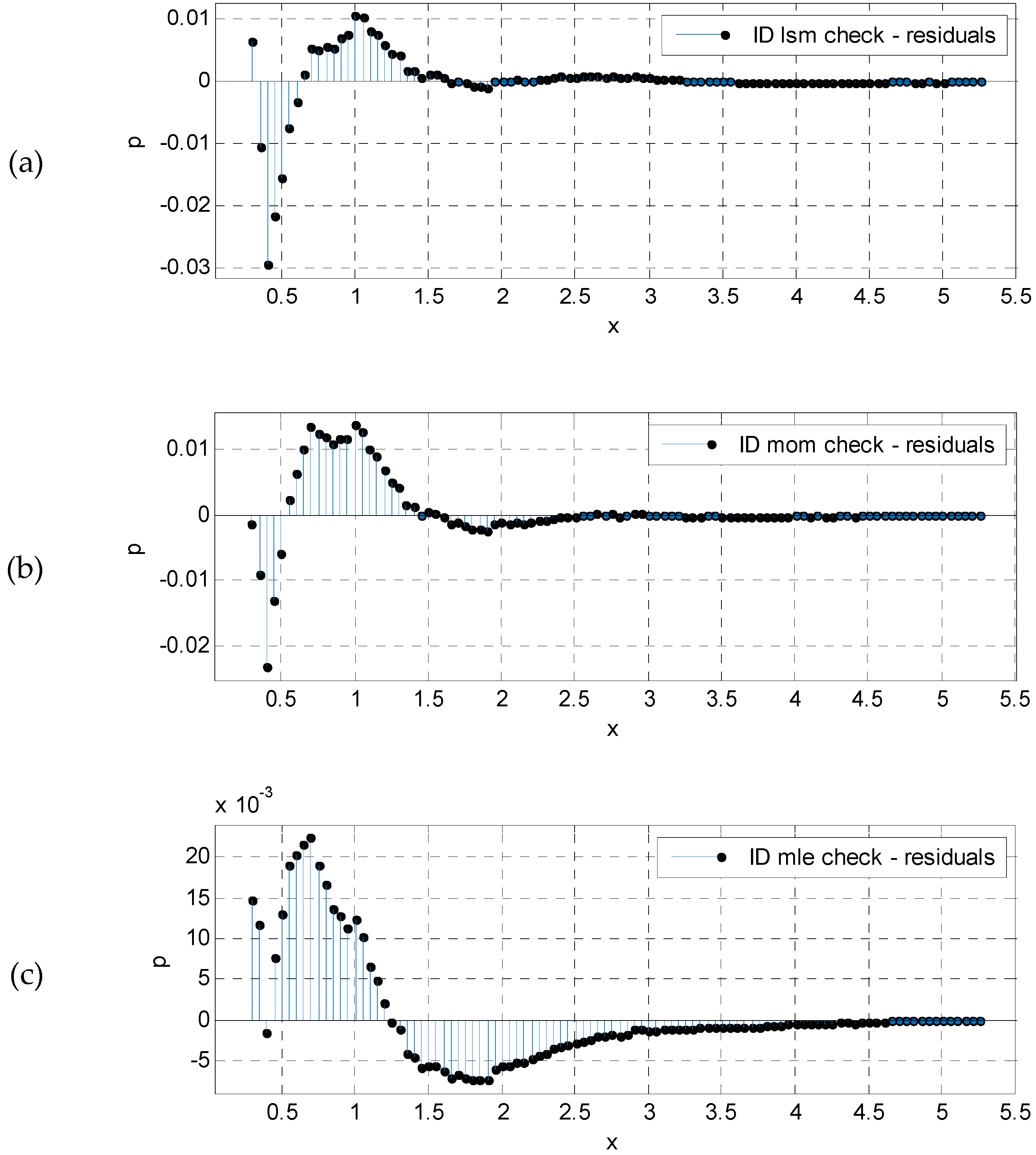
Residuals calculated and obtained by different fitting techniques are compared and presented in Figure 3.

The residuals plot (Figure 3) shows that most of the error was made for smaller wave heights, while wave heights above 2 m were very well described by the theoretical CDF. This “upper tail” of the curve was more important for extrapolating significant wave height values for return periods outside the scope of the database.

Certain limitations were noted with the MoM and MLE fitting techniques when used on this specific case study dataset for a location in the Adriatic Sea. These drawbacks are explained in the following two paragraphs.

The simultaneous optimization of all three parameters with the MoM fitting technique proved to be cumbersome. In theory, it would require the introduction of higher order moment statistics (e.g., skewness) that are more variable and more likely to result in a poor estimate [20]. Different approaches have been proposed in literature; some of them are hybrid—meaning that the proposed algorithm is a combination of the MoM and some other technique. In general, examples in the literature of fitting the three-parameter-Weibull distribution with the MoM technique are scarce. Thus, instead of performing the simultaneous optimization of all three parameters, the location parameter was set manually as the lower cut-off threshold. Significant wave heights smaller than the cut-off-threshold were discarded prior to fitting. The other two parameters were then straightforward to determine.

The MLE, expected to be superior to other techniques, proved to be inapplicable on the specific dataset due to the shape parameter β converging to a value smaller than 1. When this occurred, the probability density function approached infinity as H_s went to the value of the location parameter. This can be seen from the log likelihood function.

$$\mathsf{\Lambda }=N\ln \left(\beta \right)-N \beta \ln \left(\alpha \right)+\left(\beta -1\right){\displaystyle \sum }_{i=1}^N\ln \left(x_i-\theta \right)-{\displaystyle \sum }_{i=1}^N\left(\frac{x_i-\theta }{\alpha }\right),$$

(12)

which was to be maximized by varying the parameters. It is evident that when θ goes to x_min, ln(x_min − θ) goes to −∞; and if β is less than 1, then (β − 1)ln(x_min − α) goes to +∞. Thus, it is always possible “to find” a larger likelihood value, and convergence cannot be achieved. To avoid this issue, the lower bound of the shape parameter was set to 1. The method reached a solution, though it did so with a poorer fit compared to the LSM method. To verify this issue, ocean wave scatter diagrams available in DNV–GL (2017) were checked. It was found that the shape parameter of the three-parameter-Weibull distribution never showed values lower than 1 for the defined global nautical zones. The shape parameter was also calculated for several other locations in the Adriatic, converging to values around or lower than 1. This was, therefore, a specific problem of the local sea basin discarding the MLE fitting technique within the ID approach for the Adriatic Sea.

3.2. Annual (Monthly) Extreme Approach

The dataset extracted from the underlying database for the AM method is given in

Table 4. Yearly and monthly maximums of significant wave height [m].

Month	Year
	1993	1994	1995	1996	1997	1998	1999	2000	2001	2002	2003	2004	2005	2006	2007	2008	2009	2010	2011	2012	2013	2014	2015
1	5.26	3.07	4.11	1.94	1.54	2.21	3.08	1.75	2.94	1.52	2.99	2.44	2.21	2.21	1.62	1.67	1.92	1.33	1.58	1.22	1.72	3.06	2.53
2	2.74	3.1	1.52	2.16	1.54	1.67	2.99	1.07	3.97	2.1	2.41	2.84	1.72	1.73	1.52	1.35	2.31	3.09	2.17	2.34	3.07	2.85	2.51
3	3.87	1.7	2.82	1.28	1.12	2.08	2.73	2.62	2.73	2.12	1.71	3.03	1.32	1.95	2.7	2.29	3.38	2.42	2.42	1.42	2.74	2.29	2.29
4	1.52	2.47	1.49	1.84	2.47	1.87	3.08	2.33	2.79	3.53	2.02	1.38	2.75	1.46	1.27	1.81	3.81	1.81	1.05	1.47	1.52	1.54	1.57
5	1.57	3.57	1.47	1.15	1.47	1.62	1.36	1.63	1.42	1.87	1.75	1.81	1.1	2.07	1.28	1.49	1.1	1.95	1.62	1.89	2.74	1.4	1.49
6	1.67	2.26	2.07	1.71	1.58	1.28	1.29	1.41	2.05	2.53	0.96	1.5	1.51	1.23	1.49	0.96	1.71	1.09	1.28	1.36	0.91	1.16	1.55
7	2.68	0.92	0.83	1.18	1.29	1.29	1.65	2.74	2.37	1.95	1.46	1.27	1.15	0.8	1.9	1.2	1.63	1.41	1.23	1.52	0.81	1.36	1.74
8	2.36	1.29	1.17	1.02	1.33	2.1	1.47	0.94	2.41	1.63	2.15	1.13	0.85	2.01	0.88	0.96	1.2	1.55	1.25	1.04	1.73	1.24	1.44
9	2.6	2.34	1.73	1.87	1.99	2.18	2.84	2.29	2.58	1.6	1.97	1.81	1.97	2.36	1.6	1.44	1.68	1.3	1.17	1.49	1.35	1.64	1.69
10	3.98	2.82	1.12	3.19	2.05	1.87	3.29	2.71	1.42	2.52	3.02	1.78	1.5	1.57	1.92	2.29	2.11	2.33	1.88	2.57	1.9	1.48	2.11
11	2.71	4.26	1.86	3.89	2.66	2.73	3.16	4.05	2.62	4.43	3.11	3.02	2.63	1.77	2.09	3.57	2.63	2.83	2.31	4.56	2.34	2.82	1.74
12	3.03	4.68	2.47	2.57	2.15	2.86	3.73	1.97	3.29	2.71	2.94	1.96	2.45	1.77	1.91	3.34	2.18	2.85	2.07	1.79	3.21	2.46	1.02
Year_Max	5.26	4.68	4.11	3.89	2.66	2.86	3.73	4.05	3.97	4.43	3.11	3.03	2.75	2.36	2.7	3.57	3.81	3.09	2.42	4.56	3.21	3.06	2.53

.

The yearly maximums extracted from the underlying database represented variables to which the Gumbel distribution was to be fitted by means of the three specified fitting techniques. Monthly extremes were also reported, as they could serve for the advanced application of the AM method presented by Carter and Challenor [21]. This method allowed for the fitting of the parameter, initially for monthly extremes throughout the years (e.g., January for all 23 years, then February, and so on…); these were then summed accordingly to obtain yearly parameters to calculate extremes.

Parameters obtained by the LSM, the MoM, and the MLE are presented in

Table 5. Annual maximum (AM) approach estimated parameters for Gumbel distribution.

Parameters	LSM	MoM	MLE
α	3.1098	3.1097	3.0979
β	0.6463	0.6265	0.6404

.

Fitting with all three techniques for the AM dataset was straightforward and simple, with consistent results (very small differences) irrespective of the fitting technique applied. The LSM fit is presented on a linearized scale (WMO [6], probability paper) in Figure 4.

Goodness-of-fit values and residual plots were been checked as with the ID approach. They showed negligible differences in the order of 10E-4 between the empirical data points and the theoretical fits obtained with different fitting techniques. The differences with this order of magnitude could not be used to identify one fit superior to another.

3.3. The Peak-Over-Threshold Approach

The POT approach implies that only the peaks of clustered excesses above a certain threshold are considered [22]. These clusters represent individual storms, and their peaks represent the maximum recorded H_s of each storm. The identified storms, and their respective H_s peaks, should be independent variables so that the number of events follows a Poisson distribution, and, therefore, the interarrival time follows an exponential distribution. There are various strategies found in literature to ensure that the storms are mutually independent, e.g., [23]. A simple strategy is to define the minimum interarrival period, which is the minimum time separation between selected events, to calculate peak-to-peak (instead of threshold down-crossing to the next up-crossing). Another matter is the selection of the threshold, which is a trade-off between bias and variance: Too low a threshold is likely to violate the asymptotic basis of the model, leading to bias; too high a threshold will generate fewer excesses with which to estimate the model, leading to high variance [22]. Thus, the minimum interarrival time and the threshold were varied in order to find the optimal values. The exponential distribution shape parameter α and the respective 50-year significant wave height estimate Hs^RP are presented in Figure 5.

For the analyzed location dataset (13.50° E–45.00° N), based on the sensitivity analysis presented in Figure 5, the threshold value was set to h₀ = 2.5 m, the minimum interarrival time was set to 48 h (peak-to-peak), and the minimum duration time was set to 6 h. Similar values have been used in other extreme significant wave height studies, especially for comparable regions in the Mediterranean Sea [24]. The chosen values also corresponded to our understanding of the specific storm behavior in the Adriatic Sea, which is heavily influenced by the surrounding mountain topography. The significant wave height threshold of 2.5 m corresponded to sea state 5 (“rough”) and above according to the Douglas sea state scale dominantly used by maritime professionals. Figure 5 also clearly indicates how small differences in the selected extreme event/storm definition parameters could significantly vary the extreme estimates.

A sample time series for February 2014 is presented in Figure 6. The figure shows the variation of H_s, identified excesses of the threshold, and their respective peaks. It can be noticed (e.g., the beginning of February 2014) how only the larger of the two successive peaks attributed to the same storm event was extracted in order to satisfy the variable independence requirement.

During 23 years from the underlying database 102 storm events and respective peaks were identified. The average time between storms, d(H_s > H_s) was 323.2 records, i.e., 80.8 days. The exponential distribution parameter α, calculated by the fitting techniques methods, is presented in

Table 6. Peak-over threshold (POT) approach estimated parameter of exponential distribution.

Parameters	LSM	MoM/MLE
α	0.5931	0.5952

.

The MoM and MLE approaches yielded the same result, while the LSM fitting technique showed an insignificantly smaller value. The difference was in the order of magnitude of rounded-up error. As with the previous approaches, the LSM fit between data extracted for the POT analysis and exponential distribution was plotted on linearized WMO [6] probability paper and it presented in Figure 6.

The LSM fit, as presented in Figure 7, showed that the highest empirical data point, H_s,max = 5.26 m, was not captured well by the fit line, but it laid bellow the theoretical line. As with previous approaches, GOF values and residual plots did not indicate notable differences to suggest that one technique yielded better results than the other.

3.4. Extreme Significant Wave Height Estimation

After fitting the parameters to the candidate distribution for each approach, estimates of the significant wave height were calculated for 50- and 100-year return periods by Equations (6), (8), and (10). Additionally, values were calculated also for the 23-year return period, which was equal to the duration of the underlying database, thus rendering the calculated extreme value comparable to the maximum recorded H_s. Results are presented in

Table 7. Initial distribution approach—significant wave height estimates for 23-, 50-, and 100-year return periods.

TR [years]	HsRP–LSM [m]	HsRP–MoM [m]	HsRP–MLE [m]
23	5.77	5.44	4.87
50	6.24	5.86	5.22
100	6.65	6.23	5.53

,

Table 8. Annual maximum (extreme value) approach—significant wave height estimates for 23-, 50-, and 100-year return periods.

TR [years]	HsRP–LSM [m]	HsRP–MoM [m]	HsRP–MLE [m]
23	5.11	5.05	5.08
50	5.63	5.55	5.60
100	6.08	5.99	6.04

and

Table 9. Peak-over-threshold approach—significant wave height estimates for 23-, 50-, and 100-year return periods.

TR [years]	HsRP–LSM [m]	HsRP–MoM/MLE [m]
23 ***	5.23	5.24
50	5.69	5.70
100	6.10	6.11

*** highest H_s recorded in the underlying database was 5.26 m—this value “should” correspond to the estimated values for the 23-year return period. It is possible to notice that the variations, i.e., uncertainties were significant.

.

For the 23-year return period, which was comparable with the maximum recorded significant wave height of 5.26 m, the LSM and MoM results overestimated the targeted value, with the MoM performing better. The MLE 23-year value underestimated, but the MLE fitting technique experienced convergence limitations, with its shape parameter stopping at β = 1 and greatly affecting the results.

For the AM approach, a six-hour sea state duration was assumed for consistency with the underlying database intervals (although three-hour sea state duration is more often recommended in the literature). It is to be noted that the arbitrary “choice” of sea state duration affected the results.

The AM method provided consistent results with the different fitting techniques applied. The estimated extreme significant wave height varied up to 0.09 m for the longest, 100-year return period, implying that the fitting technique choice did not significantly affect results and can be chosen upon preference.

With the POT approach, the average number of peaks per year (calculated as 4.3 peaks-per-year) used in Equations (10) and (11) for extrapolation created an assumption that storms occurred uniformly spaced in time, which is obviously not true. The variance of the between-storms duration period could be reported in future work to illustrate this uncertainty source.

For the POT method, as the MoM and MLE techniques yielded the same result, the extreme significant wave height was also the same. The results obtained by LSM and MoM/MLE differed by less than 0.01 m, making POT the most consistent compared to other approaches.

Overall, the largest difference at the analyzed location (13.5° E–45.0° N) was found between the ID-LSM and the AM-MoM result, if ID-MLE is not considered due to its mathematical limitation. The 23-year return period showed that the best fit to the maximum recorded value from the underlying database (5.26 m) was obtained by the POT approach, with virtually no difference based on the fitting technique.

4. Discussion on Accuracy Evaluation Including Spatial Considerations

The analysis was extended to consider spatial variability. The same methodology, described in earlier sections, was applied to locations in central and south Adriatic Sea, with their respective geographical coordinates of 15.5° E–43.0° N and 17.5° E–41.5° N. Both locations are located offshore on a busy shipping route [3]. For the POT method, based on different input data and the POT parameter analysis (similar to that in Section 3.3), the threshold for the two additional locations was set to h₀ = 3.2 m, while the minimum interarrival time (defined simplified as peak-to-peak) remained 48 h. Minimum storm duration was defined as 6 h, corresponding to one record in the underlaying database. Considering the chosen high threshold (H_s > 2.5 (3.2) m), six hours was considered to be a representative storm duration in the Adriatic Sea. The same minimum storm duration has been used in other studies for the Mediterranean Sea [24].

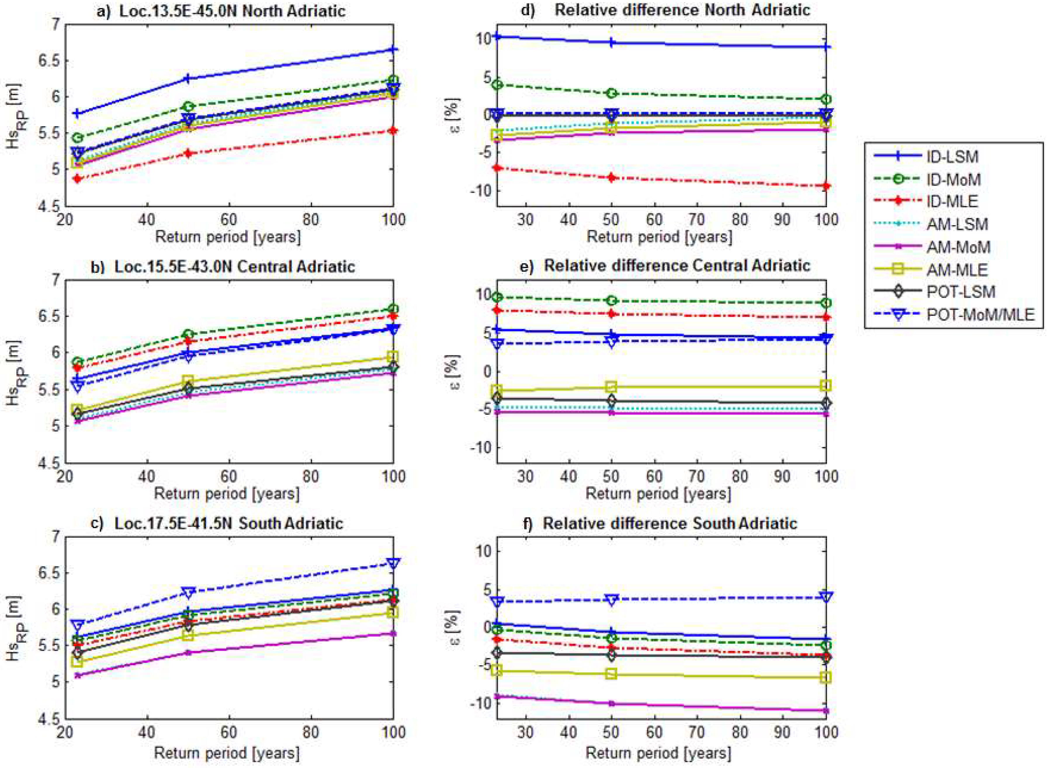
The results of significant wave height estimations for long return periods obtained with analyzed approaches are presented in Figure 8, with their mutual relative trends. Based on the obtained numerical results, the average of the two POT curves was used as a reference value H_s,ref. Thus, the mutual trend of other approaches and techniques, H_s,i^RP, was calculated according to:

$$\epsilon =\frac{H_{S,i}^{RP}-H_{S,ref}}{H_{S,ref}}\times 100,$$

(13)

The results indicated that significant differences could be expected due to the selected approach. Moreover, differences were evident for the same approach depending on the fitting technique due to very small differences between the obtained parameters.

The average values of results obtained for each return period (ID-MLE excluded) and respective standard deviations were as follows: H_s^RP=23y = 5.28 m (stand. dev. = 0.25); H_s^RP=50y = 5.75 m (stand. dev. = 0.24); and H_s^RP=100y = 6.17 m (stand. dev. = 0.22).

If all three analyzed locations are considered, a relatively constant bias, in the order of magnitude of about +/−0.5 meter (+/−10%) with respect to the average of extreme values, was evident between results obtained by various methods (the ID-MLE excluded for the north Adriatic location because it was, in fact, inapplicable for the specific dataset). Various approaches and fitting techniques seemed to cluster around the same mean value. Based on this, it was possible to give a recommendation to engineers to always use multiple approaches when possible in order to verify the results when developing such an analysis.

For the specific and relatively large dataset (23 years with no gaps), the AM and POT approaches in combination with the LSM fitting technique proved to be the most consistent.

The ID approach is straightforward but influenced by the smaller wave height, and bulk data points can fail to capture the upper fit tail (highest H_s), which is especially important for extrapolation to long return periods. This could be countered by employing other goodness-of-fit tests, such as the Anderson–Darling test, which is devised to give heavier weight to the tails.

It should be mentioned that the return period calculation with the AM approach depends on the assumption of the sea state duration Δt. The choice can be made arbitrarily. A common choice is to use the same interval as in the underlying database for consistency (six-hour in this study) or accept and recalculate to Δt = three-hour interval, which is more widely suggested in literature (DNV–GL [7]). The choice influences the results.

For the POT method, the crucial parameters are: the selection of the threshold and interarrival time between storms. The selection of these parameters will lead to very different results regarding the fits and the return period estimates.

Finally, a manual “fit-by-eye” subjective fitting technique (as opposite to “objective” mathematical approaches) is worth mentioning. Some authors (e.g., Holthuijsen [5]) have argued that, if made by an experienced engineer, this approach can possibly give better results since the engineer can weigh the importance of empirical points at his own discretion, disregarding or emphasizing certain wave heights depending on the intended use of the analyses.

The variability of wind-wave directionality can affect the extreme value estimation, so the assumption of the performed univariate analysis implies equal probability of extremes arriving from all directions during all seasons and wind patterns with averaged characteristics. This presents a simplification of the problem. Specifically, for the Adriatic Sea, the analysis could be refined by separating the calculation of the extremes by dominant regional wind patterns. Most wave extremes occur from south-eastern winds (jugo, sirocco) that develop gradually, build up, and last longer in contrast to the north-eastern winds (bura, bora), which can occur very suddenly and violently but are fetch limited. These wind patterns and accompanying waves have different characteristics and consequently represent statistically separate datasets. Thus, for future work, the individual analysis of the extremes caused by distinguishable wind patterns of jugo and bura are expected to yield more accurate predictions.

5. Conclusions

The paper systematically analyzed major approaches and fitting techniques, according to relevant engineering practice, in order to estimate significant wave heights for 50- and 100-year return periods in a case study for three locations in the Adriatic Sea (north, central, and south). The analysis was based on a 23-year database of wave measurement and numerical modelling. The initial-distribution approach employed the three-parameter-Weibull distribution, the annual-maximum approach was assumed to follow the Gumbel distribution, and the dataset extracted for the peak-over-threshold was described by the exponential distribution. Theoretical distribution fit parameters were estimated by means of the least-mean-square method, the method-of-moments, and the maximum-likelihood fitting techniques. The problems encountered for the dataset concerning the specific case study are reported, and the causes of results variability noted. After obtaining various fits, the significant wave height was evaluated for 23-, 50-, and 100-year return periods. The calculated 23-year return period allowed for a comparison with the maximum recorded significant wave height in the underlying database. Differences between methods showed a relatively constant bias that did not depend on the return period. Significant differences can occur depending on the choice of model and parameter fitting technique. For the analyzed dataset, this was in the order of magnitude of 0.5 m. If the intended use of the analysis of extremes is an input for the engineering of offshore structures, such variability can greatly affect cost and safety.

Various uncertainty causes were identified, and these make it a reasonable suggestion to check different approaches whenever possible.