A Tidal Hydrodynamic Model for Cook Inlet, Alaska, to Support Tidal Energy Resource Characterization


Abstract
:1. Introduction
2. Methods
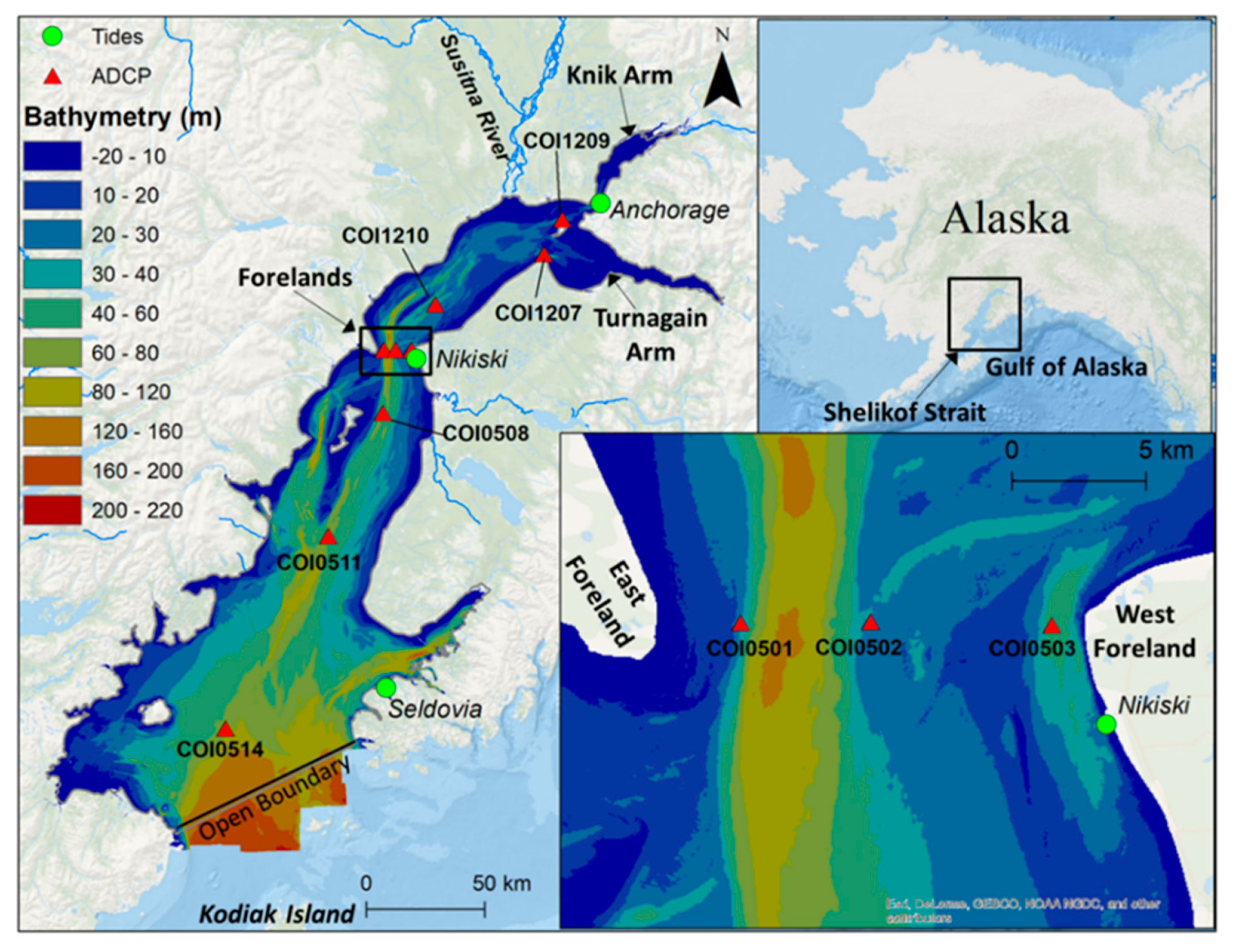
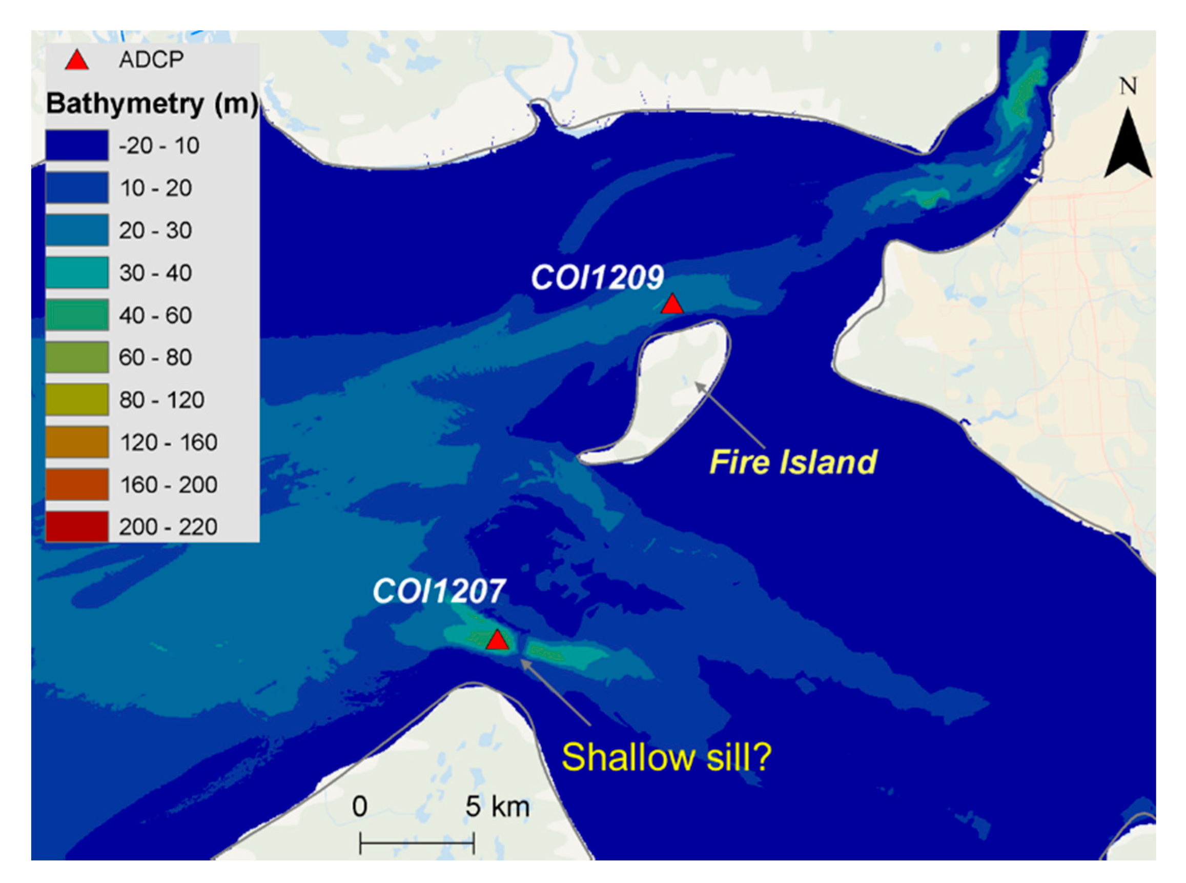
2.1. Study Site
2.2. Hydrodynamic Model
2.3. Model Configuration
3. Results and Discussion
3.1. Model Calibration
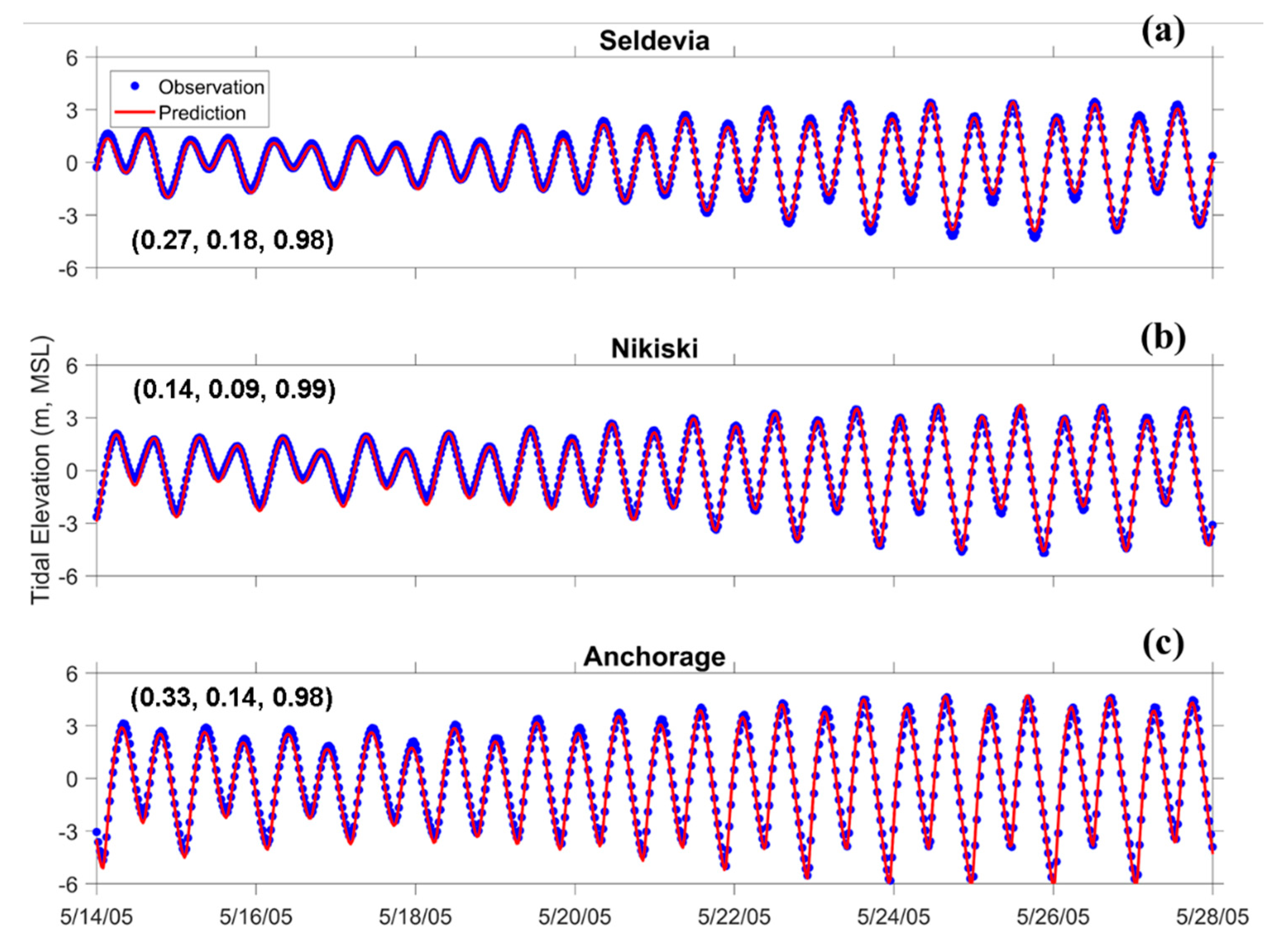
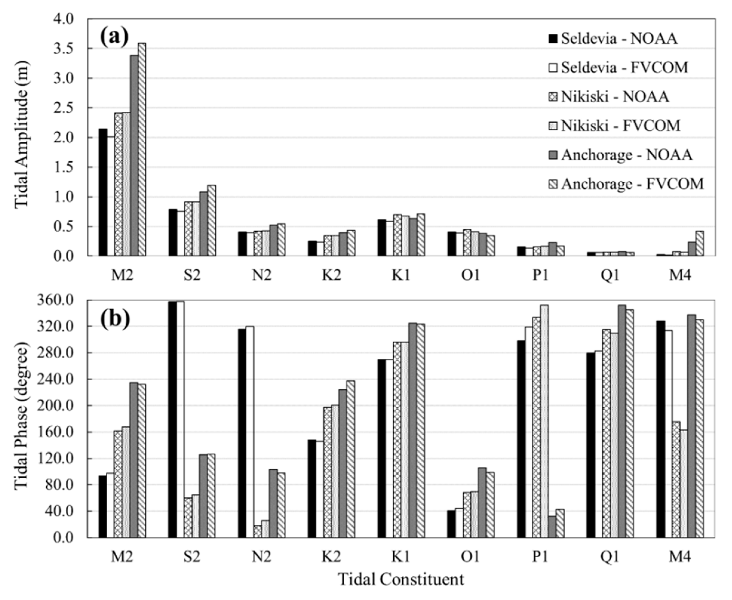
3.1.1. Tidal Elevation
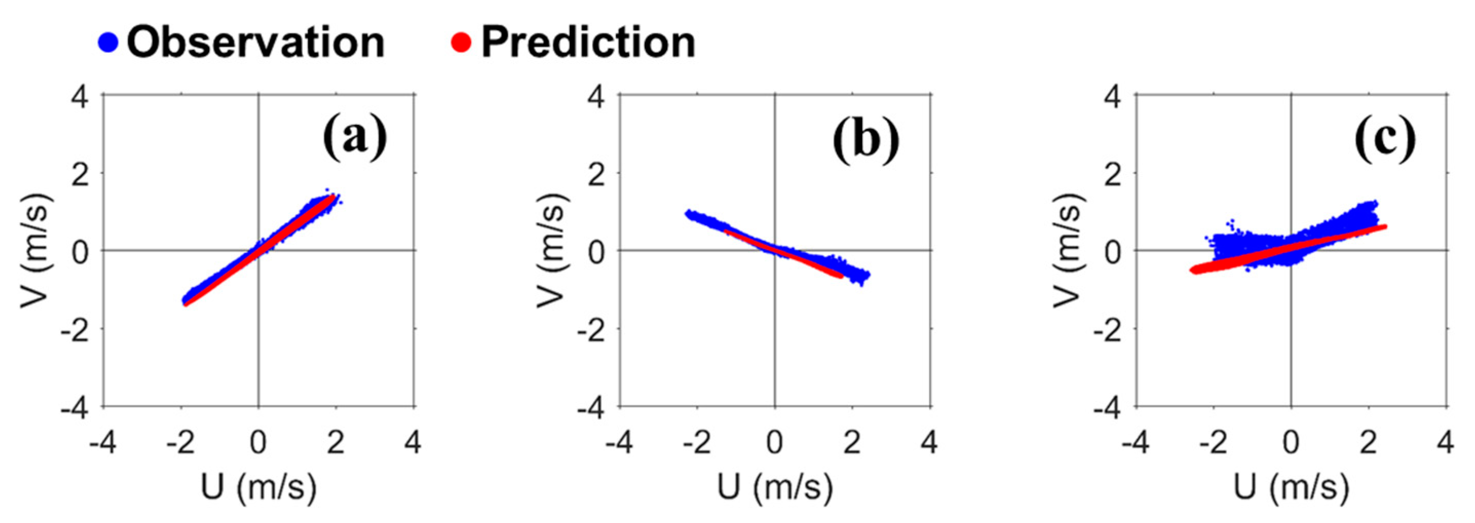
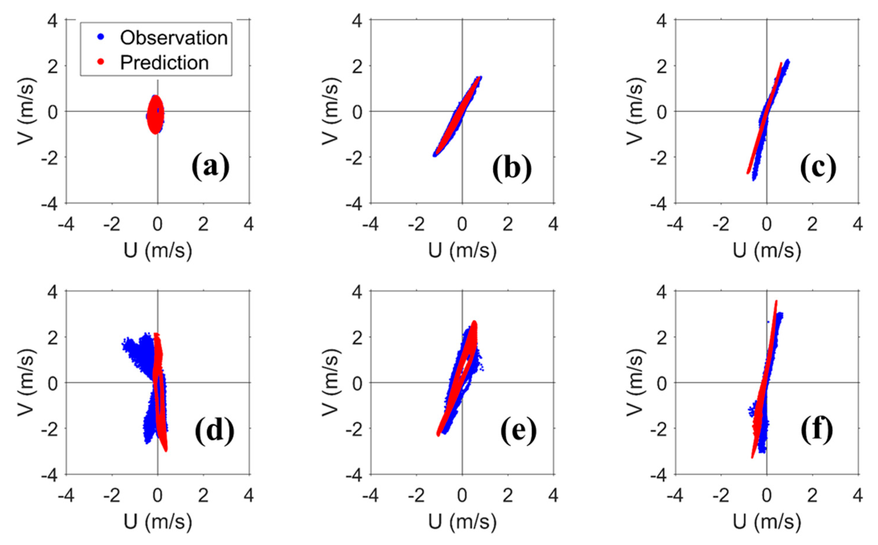
3.1.2. Tidal Velocity
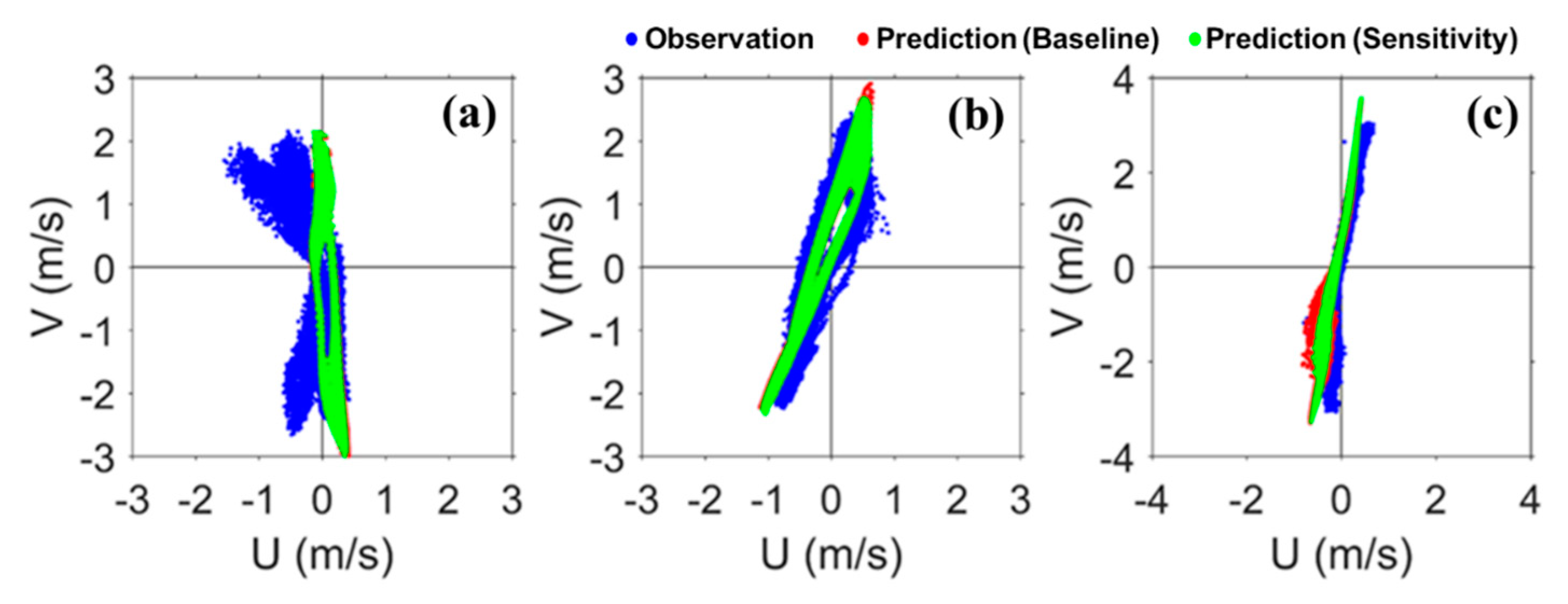
3.2. A Sensitivity Test on the Effect of Grid Resolution
3.3. Model Validation
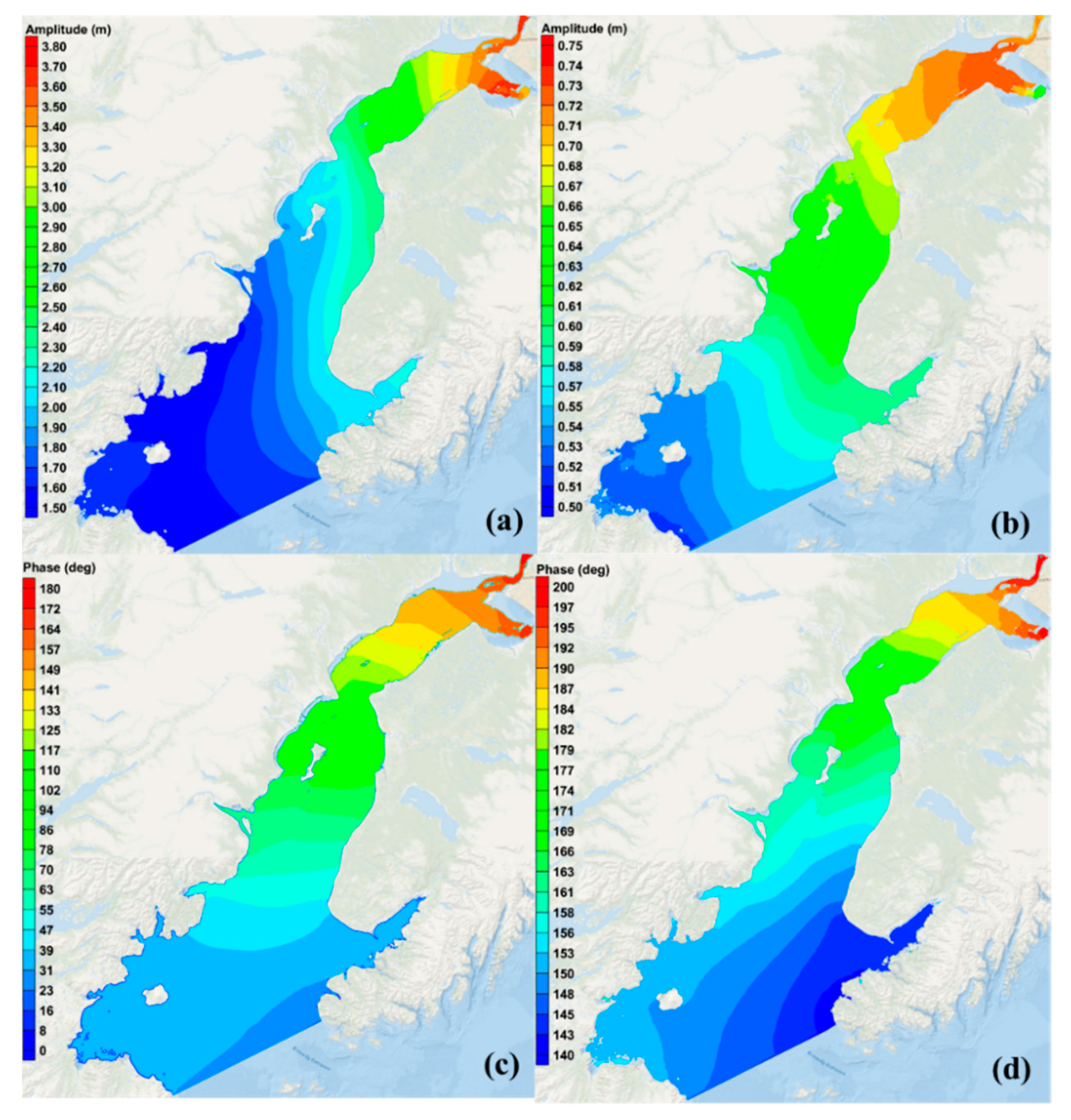
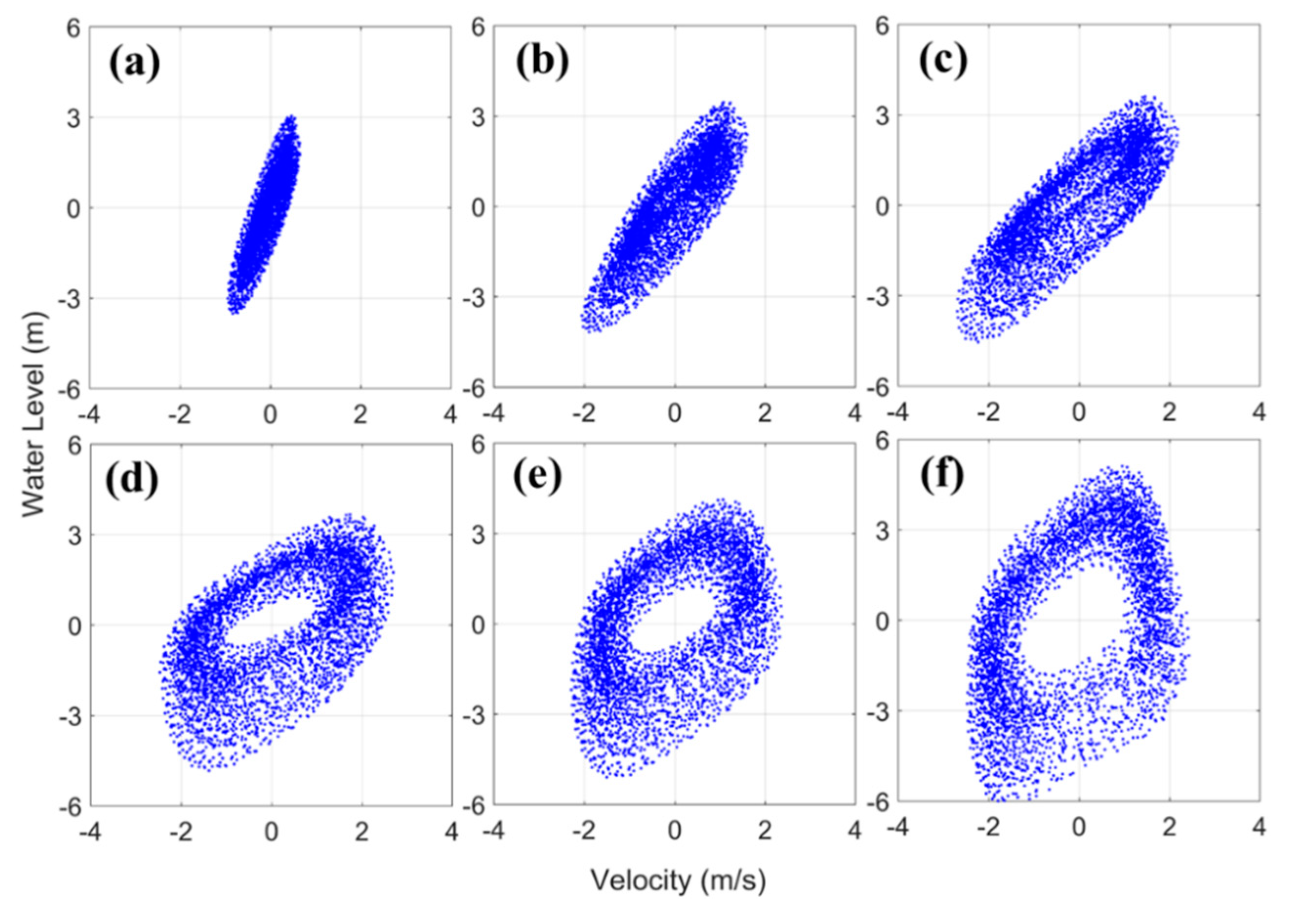
3.4. Tidal Characteristics
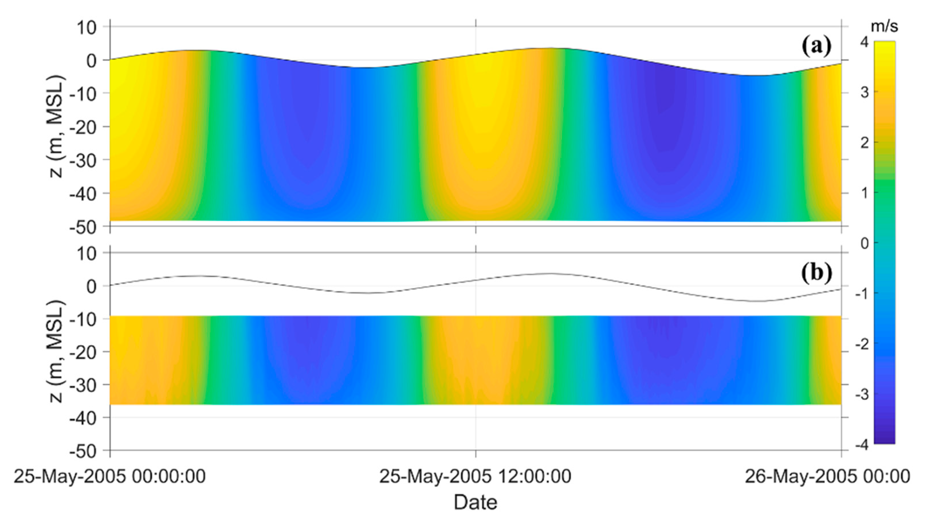
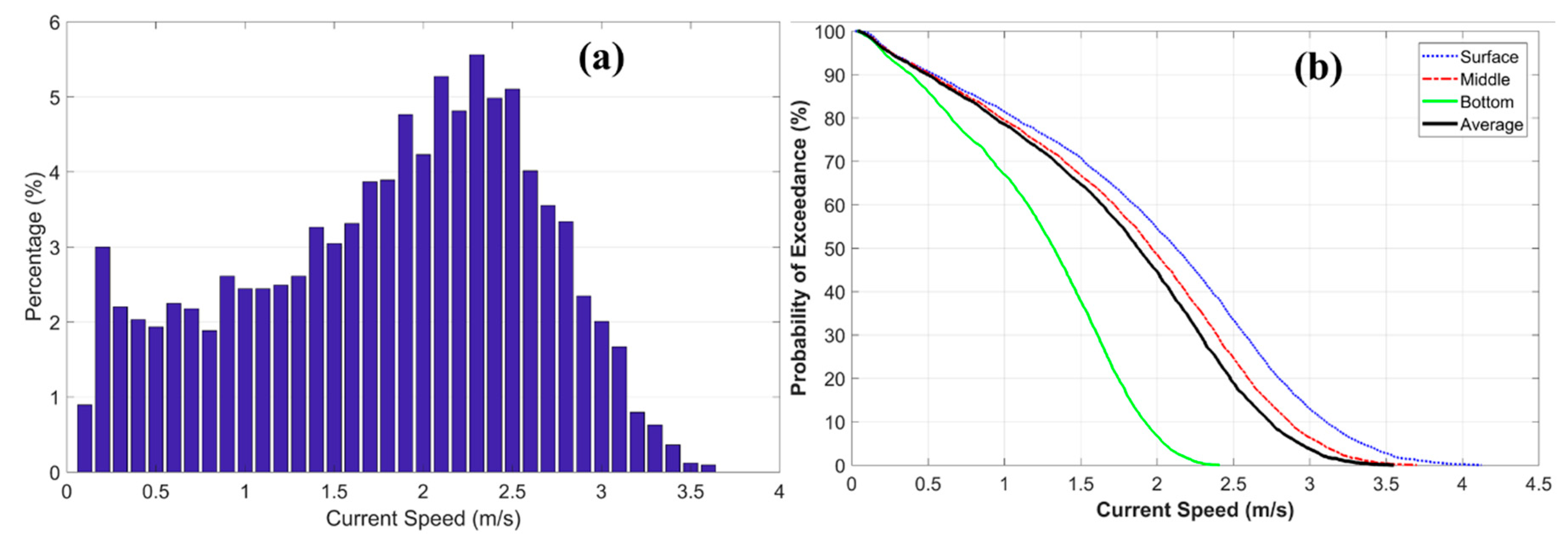
3.5. Spatial Variability of Tidal Currents
3.6. Tidal Energy Extraction Potential in Cook Inlet
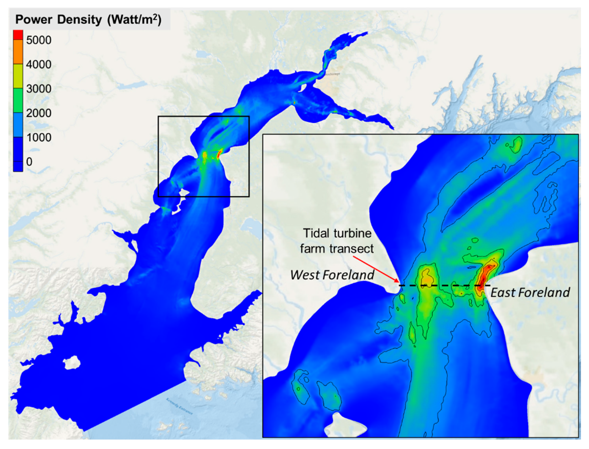
3.6.1. Tidal Energy Resource Distribution
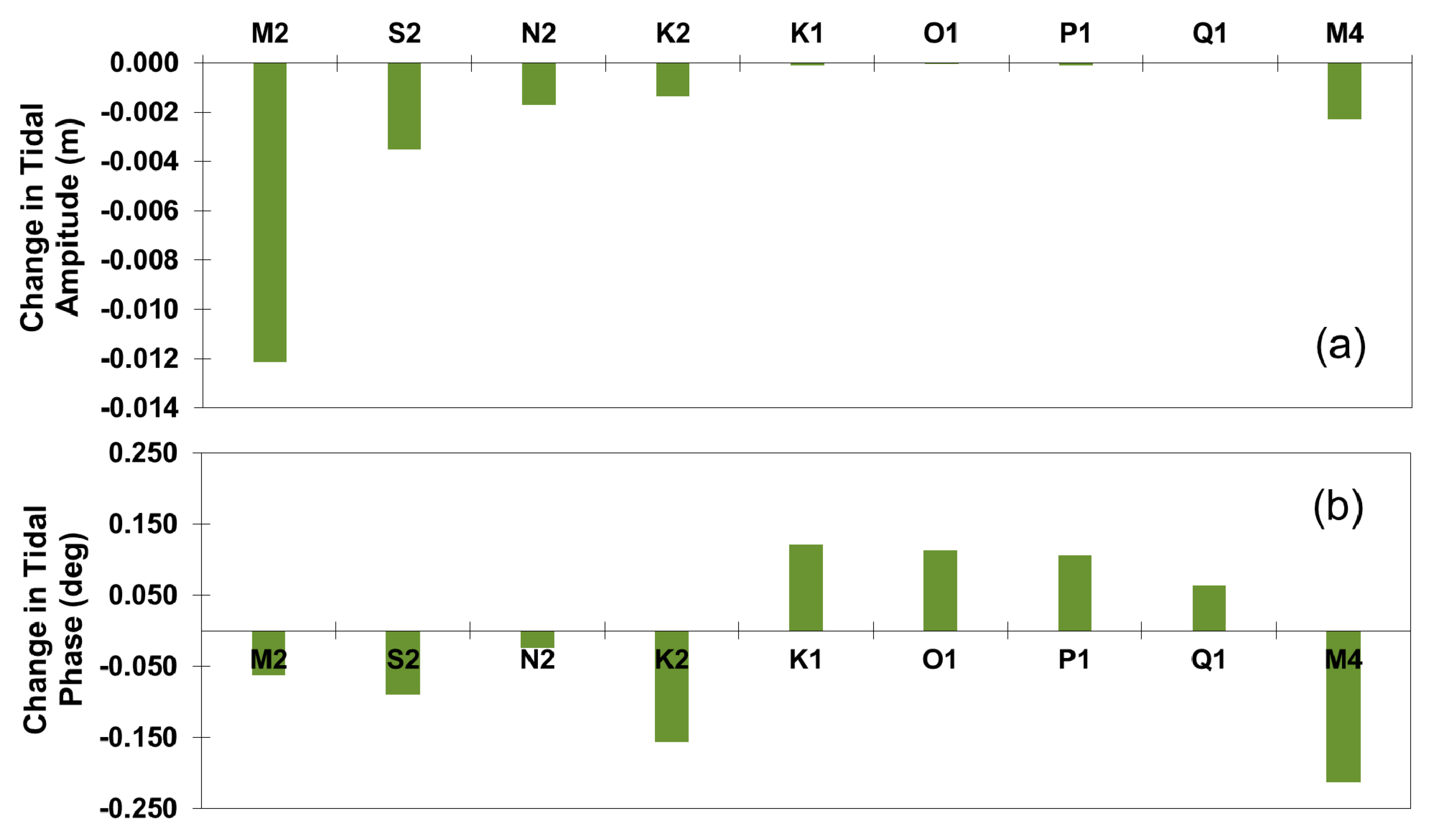
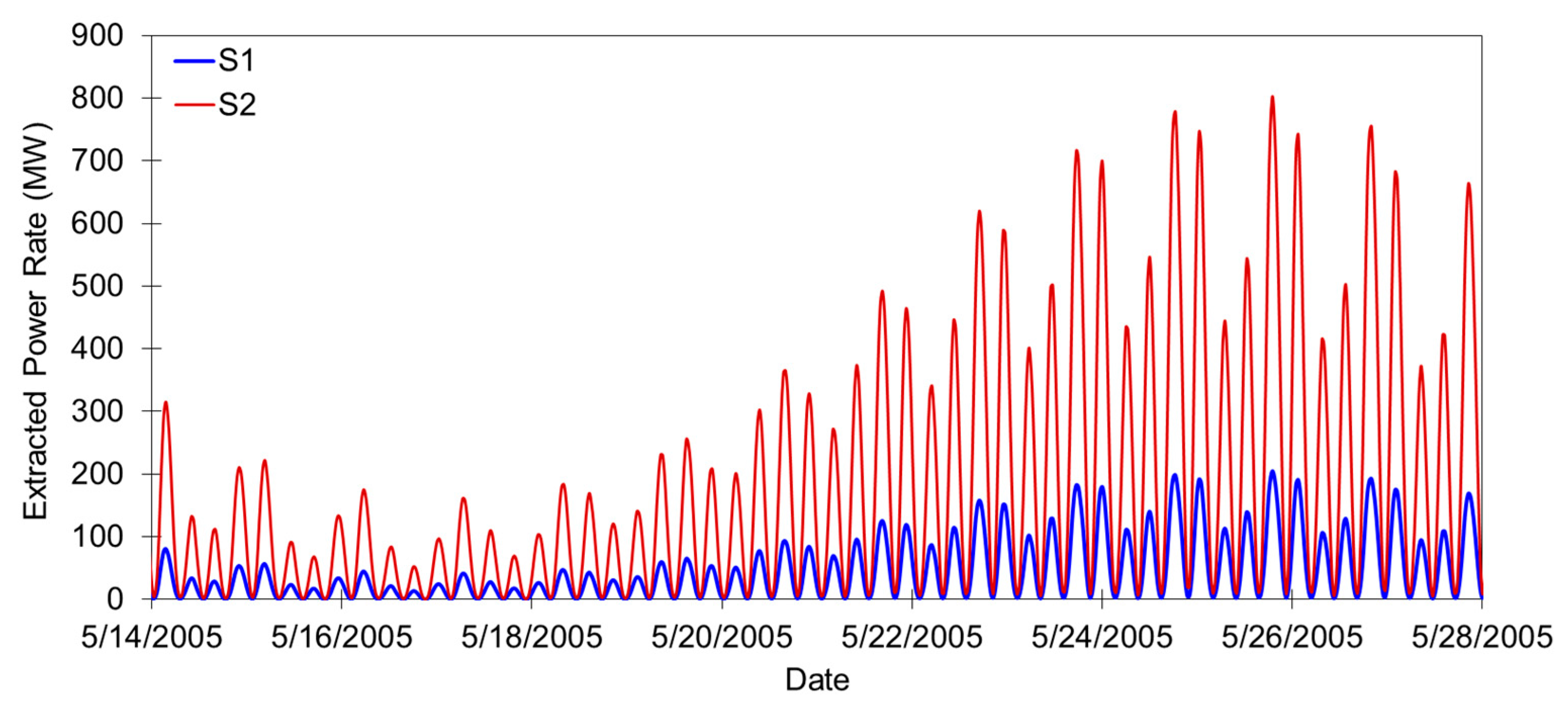
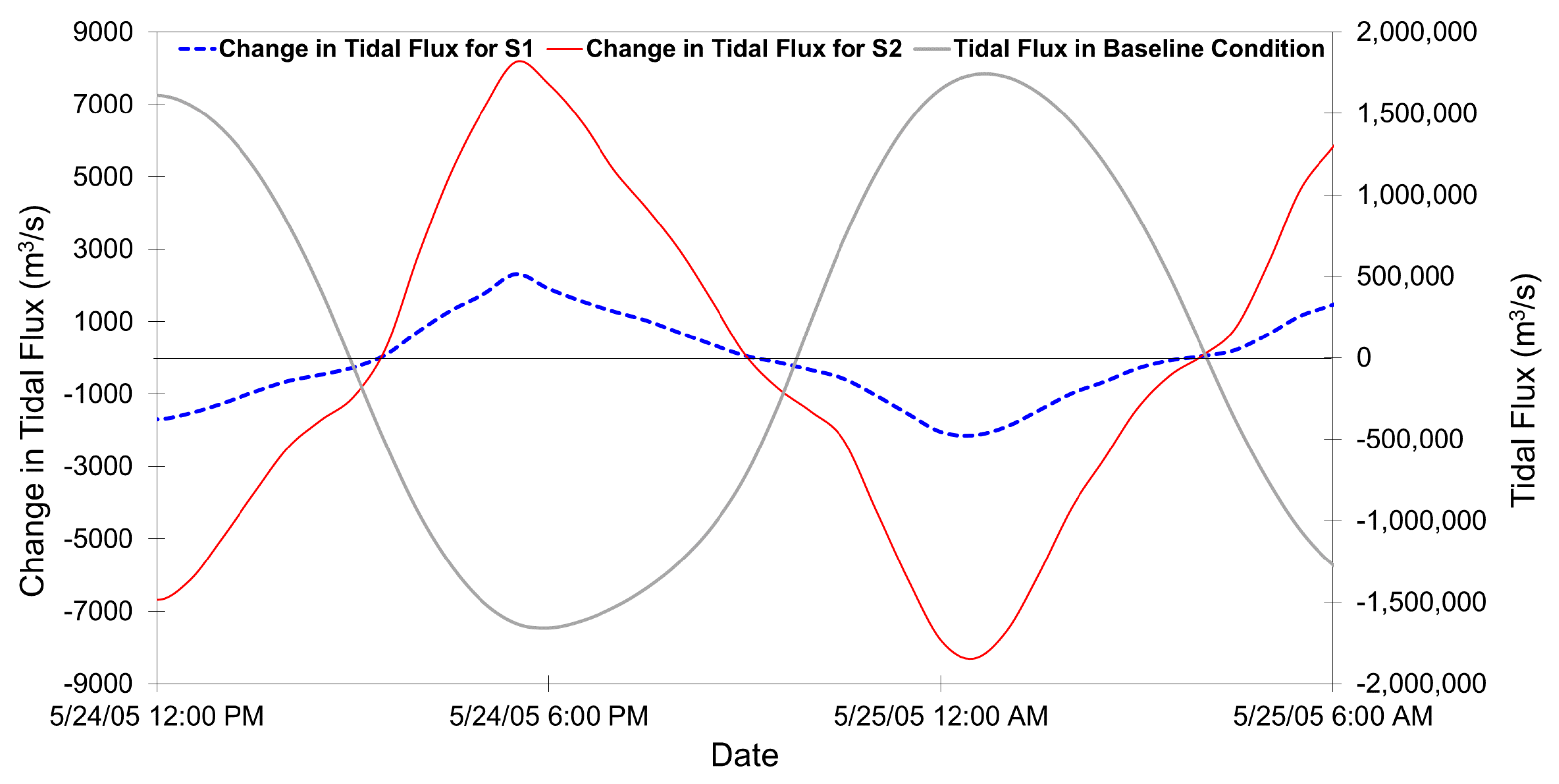
3.6.2. Assessing Tidal Energy Extraction Potential
4. Summary
Author Contributions
Funding
Acknowledgments
Conflicts of Interest
References
- Blunden, L.S.; Bahaj, A.S. Initial evaluation of tidal stream energy resources at Portland Bill, UK. Renew. Energy 2006, 31, 121–132. [Google Scholar] [CrossRef]
- Grabbe, M.; Lalander, E.; Lundin, S.; Leijon, M. A review of the tidal current energy resource in Norway. Renew. Sustain. Energy Rev. 2009, 13, 1898–1909. [Google Scholar] [CrossRef] [Green Version]
- Lewis, M.; McNaughton, J.; Márquez-Dominguez, C.; Todeschini, G.; Togneri, M.; Masters, I.; Allmark, M.; Stallard, T.; Neill, S.; Goward-Brown, A.; et al. Power variability of tidal-stream energy and implications for electricity supply. Energy 2019, 183, 1061–1074. [Google Scholar] [CrossRef]
- O’Carroll, J.P.J.; Kennedy, R.M.; Creech, A.; Savidge, G. Tidal Energy: The benthic effects of an operational tidal stream turbine. Mar. Environ. Res. 2017, 129, 277–290. [Google Scholar] [CrossRef]
- Hasegawa, D.; Sheng, J.; Greenberg, D.A.; Thompson, K.R. Far-field effects of tidal energy extraction in the Minas Passage on tidal circulation in the Bay of Fundy and Gulf of Maine using a nested-grid coastal circulation model. Ocean Dyn. 2011, 61, 1845–1868. [Google Scholar] [CrossRef]
- Lewis, M.; Neill, S.P.; Robins, P.E.; Hashemi, M.R. Resource assessment for future generations of tidal-stream energy arrays. Energy 2015, 83, 403–415. [Google Scholar] [CrossRef] [Green Version]
- Goward Brown, A.J.; Neill, S.P.; Lewis, M.J. Tidal energy extraction in three-dimensional ocean models. Renew. Energy 2017, 114, 244–257. [Google Scholar] [CrossRef] [Green Version]
- Mejia-Olivares, C.J.; Haigh, I.D.; Wells, N.C.; Coles, D.S.; Lewis, M.J.; Neill, S.P. Tidal-stream energy resource characterization for the Gulf of California, México. Energy 2018, 156, 481–491. [Google Scholar] [CrossRef]
- Ward, S.L.; Robins, P.E.; Lewis, M.J.; Iglesias, G.; Hashemi, M.R.; Neill, S.P. Tidal stream resource characterisation in progressive versus standing wave systems. Appl. Energy 2018, 220, 274–285. [Google Scholar] [CrossRef]
- Yang, Z.; Wang, T.; Copping, A.E. Modeling tidal stream energy extraction and its effects on transport processes in a tidal channel and bay system using a three-dimensional coastal ocean model. Renew. Energy 2013, 50, 605–613. [Google Scholar] [CrossRef]
- Yang, Z.; Wang, T.; Copping, A.; Geerlofs, S. Modeling of in-stream tidal energy development and its potential effects in Tacoma Narrows, Washington, USA. Ocean Coast. Manag. 2014, 99, 52–62. [Google Scholar] [CrossRef]
- MeyGen Project. Available online: https://simecatlantis.com/projects/meygen/ (accessed on 11 November 2019).
- Verdant Power. Available online: https://www.verdantpower.com/ (accessed on 11 November 2019).
- Neary, V.S.; Gunawan, B.; Hill, C.; Chamorro, L.P. Near and far field flow disturbances induced by model hydrokinetic turbine: ADV and ADP comparison. Renew. Energy 2013, 60, 1–6. [Google Scholar] [CrossRef]
- Defne, Z.; Haas, K.A.; Fritz, H.M. Numerical modeling of tidal currents and the effects of power extraction on estuarine hydrodynamics along the Georgia coast, USA. Renew. Energy 2011, 36, 3461–3471. [Google Scholar] [CrossRef]
- Richmond, M.; Harding, S.; Romero-Gomez, P. Numerical performance analysis of acoustic Doppler velocity profilers in the wake of an axial-flow marine hydrokinetic turbine. Int. J. Mar. Energy 2015, 11, 50–70. [Google Scholar] [CrossRef] [Green Version]
- Haas, K.A.; Fritz Hermann, M.; French Steven, P.; Smith Brennan, T.; Neary, V. Assessment of Energy Production Potential from Tidal Streams in the United States; Tech Research Corporation: Atlanta, GA, USA, 2011. [Google Scholar] [CrossRef] [Green Version]
- Martin-Short, R.; Hill, J.; Kramer, S.C.; Avdis, A.; Allison, P.A.; Piggott, M.D. Tidal resource extraction in the Pentland Firth, UK: Potential impacts on flow regime and sediment transport in the Inner Sound of Stroma. Renew. Energy 2015, 76, 596–607. [Google Scholar] [CrossRef] [Green Version]
- Thiébot, J.; Bailly du Bois, P.; Guillou, S. Numerical modeling of the effect of tidal stream turbines on the hydrodynamics and the sediment transport–Application to the Alderney Race (Raz Blanchard), France. Renew. Energy 2015, 75, 356–365. [Google Scholar] [CrossRef]
- Wang, T.; Yang, Z. A modeling study of tidal energy extraction and the associated impact on tidal circulation in a multi-inlet bay system of Puget Sound. Renew. Energy 2017, 114, 204–214. [Google Scholar] [CrossRef]
- Karsten, R.H.; McMillan, J.M.; Lickley, M.J.; Haynes, R.D. Assessment of tidal current energy in the Minas Passage, Bay of Fundy. Proc. Inst. Mech. Eng. Part A J. Power Energy 2008, 222, 493–507. [Google Scholar] [CrossRef]
- Neill, S.P.; Litt, E.J.; Couch, S.J.; Davies, A.G. The impact of tidal stream turbines on large-scale sediment dynamics. Renew. Energy 2009, 34, 2803–2812. [Google Scholar] [CrossRef]
- Karsten, R.; Swan, A.; Culina, J. Assessment of arrays of in-stream tidal turbines in the Bay of Fundy. Philos. Trans. A Math. Phys. Eng. Sci. 2013, 371, 20120189. [Google Scholar] [CrossRef] [Green Version]
- Ramos, V.; Carballo, R.; Álvarez, M.; Sánchez, M.; Iglesias, G. Assessment of the impacts of tidal stream energy through high-resolution numerical modeling. Energy 2013, 61, 541–554. [Google Scholar] [CrossRef]
- Nash, S.; O’Brien, N.; Olbert, A.; Hartnett, M. Modelling the far field hydro-environmental impacts of tidal farms – A focus on tidal regime, inter-tidal zones and flushing. Comput. Geosci. 2014, 71, 20–27. [Google Scholar] [CrossRef]
- Rao, S.; Xue, H.; Bao, M.; Funke, S. Determining tidal turbine farm efficiency in the Western Passage using the disc actuator theory. Ocean Dyn. 2015, 66, 41–57. [Google Scholar] [CrossRef]
- State of Alaska, Officer of the Governor. Preliminary assessment of Cook Inlet Tidal Power. Phase 1 Rep. 1981, 1, 97. [Google Scholar]
- Kilcher, L.; Thresher, R. Marine Hydrokinetic Energy Site Identification and Ranking Methodology Part II: Tidal Energy. 2016; 30. Available online: https://www.nrel.gov/docs/fy17osti/66079.pdf (accessed on 4 April 2020).
- Chen, C.; Liu, H.; Beardsley, R.C. An Unstructured Grid, Finite-Volume, Three-Dimensional, Primitive Equations Ocean Model: Application to Coastal Ocean and Estuaries. J. Atm. Ocean. Tech. 2003, 20, 159–186. [Google Scholar] [CrossRef]
- Chen, C.B.; Robert, C.; Cowles, G. An unstructured grid, finite-volume coastal ocean model (FVCOM) system. Oceanography 2006, 19, 78–89. [Google Scholar] [CrossRef] [Green Version]
- Chen, C.; Xu, Q.; Houghton, R.; Beardsley, R.C. A model-dye comparison experiment in the tidal mixing front zone on the southern flank of Georges Bank. J. Geophys. Res. 2008, 113. [Google Scholar] [CrossRef] [Green Version]
- Xuan, J.; Yang, Z.; Huang, D.; Wang, T.; Zhou, F. Tidal residual current and its role in the mean flow on the Changjiang Bank. J. Mar. Syst. 2016, 154, 66–81. [Google Scholar] [CrossRef]
- Lai, Z.; Ma, R.; Gao, G.; Chen, C.; Beardsley, R.C. Impact of multichannel river network on the plume dynamics in the Pearl River estuary. J. Geophys. Res. Ocean. 2015, 120, 5766–5789. [Google Scholar] [CrossRef] [Green Version]
- Wang, T.; Khangaonkar, T.; Long, W.; Gill, G. Development of a Kelp-Type Structure Module in a Coastal Ocean Model to Assess the Hydrodynamic Impact of Seawater Uranium Extraction Technology. J. Mar. Sci. Eng. 2014, 2, 81–92. [Google Scholar] [CrossRef]
- Yang, Z.; Wang, T. Modeling the Effects of Tidal Energy Extraction on Estuarine Hydrodynamics in a Stratified Estuary. Estuaries Coasts 2013, 38, 187–202. [Google Scholar] [CrossRef]
- Wang, T.; Yang, Z.; Copping, A. A Modeling Study of the Potential Water Quality Impacts from In-Stream Tidal Energy Extraction. Estuaries Coasts 2013, 38, 173–186. [Google Scholar] [CrossRef]
- Zimmermann, M.P.; Megan, M. AFSC/RACE: Cook Inlet Grid. 2014. Available online: http://www.afsc.noaa.gov/RACE/groundfish/bathymetry/Cook_bathymetry_grid.zip (accessed on 4 April 2020).
- Chen, C.; Beardsley, R.C.; Cowles, G. An unstructured grid, finite-volume coastal ocean model: FVCOM user manual. School for Marine Science and Technology. Oceanography 2006, 19, 78. [Google Scholar] [CrossRef] [Green Version]
- Egbert, G.D.E.; Svetlana, Y. Efficient Inverse Modeling of Barotropic Ocean Tides. J. Atmos. Ocean. Technol. 2002, 19, 183–204. [Google Scholar] [CrossRef] [Green Version]
- International Electrotechnical Commission. Tidal Energy Resource Assessment and Characterization (Technical Specification No. 62600-201), Marine Energy-WAVE, Tidal and Other Water Current Converters; IEC: Geneva, Switzerland, 2015; p. 46. [Google Scholar]
- Oey, L.-Y.; Ezer, T.; Hu, C.; Muller-Karger, F.E. Baroclinic tidal flows and inundation processes in Cook Inlet, Alaska: Numerical modeling and satellite observations. Ocean Dyn. 2007, 57, 205–221. [Google Scholar] [CrossRef]


| Station | Sample Year | Longitude | Latitude | Depth (m) | # of Bins | Station Full Name |
|---|---|---|---|---|---|---|
| COI0514 | 2005 | −152.93028 | 59.30180 | 80.2 | 20 | Augustine Island |
| COI0511 | 2005 | −152.12018 | 60.02327 | 68.6 | 18 | Cape Ninilchik, west of |
| COI0508 | 2005 | −151.67325 | 60.48295 | 51.5 | 11 | Kalgin Island, east of |
| COI0501 | 2005 | −151.64690 | 60.72198 | 33.5 | 9 | West Foreland |
| COI0502 | 2005 | −151.55733 | 60.72067 | 33.8 | 7 | The Forelands |
| COI0503 | 2005 | −151.43297 | 60.71727 | 44.2 | 12 | East Foreland |
| COI1210 | 2012 | −151.23268 | 60.88697 | 43.3 | 15 | Middle Ground Shoal, east of |
| COI1207 | 2002 | −150.36035 | 61.05660 | 53.3 | 19 | Point Possession |
| COI1209 | 2012 | −150.20150 | 61.18483 | 29.4 | 15 | Fire Island, north of |
| Station | Vel. Comp | COI 0514 | COI 0511 | COI 0508 | COI 0501 | COI 0502 | COI 0503 |
|---|---|---|---|---|---|---|---|
| RMSE (m/s) | U | 0.07 | 0.09 | 0.13 | 0.45 | 0.15 | 0.17 |
| V | 0.08 | 0.11 | 0.20 | 0.24 | 0.17 | 0.31 | |
| SI | U | 0.62 | 0.23 | 0.43 | 1.35 | 0.42 | 0.82 |
| V | 0.29 | 0.17 | 0.18 | 0.20 | 0.14 | 0.18 | |
| R2 | U | 0.85 | 0.97 | 0.92 | 0.19 | 0.93 | 0.90 |
| V | 0.95 | 0.98 | 0.98 | 0.98 | 0.99 | 0.99 |
| Station | Vel. Comp | COI 0501 | COI 0502 | COI 0503 |
|---|---|---|---|---|
| RMSE (m/s) | U | 0.45 | 0.15 | 0.19 |
| V | 0.24 | 0.17 | 0.23 | |
| SI | U | 1.37 | 0.42 | 0.90 |
| V | 0.20 | 0.14 | 0.18 | |
| R2 | U | 0.19 | 0.93 | 0.90 |
| V | 0.98 | 0.99 | 0.99 |
| Station | Vel. Comp | COI 1210 | COI 1207 | COI 1209 |
|---|---|---|---|---|
| RMSE (m/s) | U | 0.12 | 0.58 | 0.37 |
| V | 0.12 | 0.23 | 0.38 | |
| SI | U | 0.11 | 0.42 | 0.30 |
| V | 0.16 | 0.48 | 1.0 | |
| R2 | U | 0.99 | 0.97 | 0.97 |
| V | 0.99 | 0.97 | 0.57 |
© 2020 by the authors. Licensee MDPI, Basel, Switzerland. This article is an open access article distributed under the terms and conditions of the Creative Commons Attribution (CC BY) license (http://creativecommons.org/licenses/by/4.0/).
Share and Cite
Wang, T.; Yang, Z. A Tidal Hydrodynamic Model for Cook Inlet, Alaska, to Support Tidal Energy Resource Characterization. J. Mar. Sci. Eng. 2020, 8, 254. https://doi.org/10.3390/jmse8040254
Wang T, Yang Z. A Tidal Hydrodynamic Model for Cook Inlet, Alaska, to Support Tidal Energy Resource Characterization. Journal of Marine Science and Engineering. 2020; 8(4):254. https://doi.org/10.3390/jmse8040254
Chicago/Turabian StyleWang, Taiping, and Zhaoqing Yang. 2020. "A Tidal Hydrodynamic Model for Cook Inlet, Alaska, to Support Tidal Energy Resource Characterization" Journal of Marine Science and Engineering 8, no. 4: 254. https://doi.org/10.3390/jmse8040254
APA StyleWang, T., & Yang, Z. (2020). A Tidal Hydrodynamic Model for Cook Inlet, Alaska, to Support Tidal Energy Resource Characterization. Journal of Marine Science and Engineering, 8(4), 254. https://doi.org/10.3390/jmse8040254