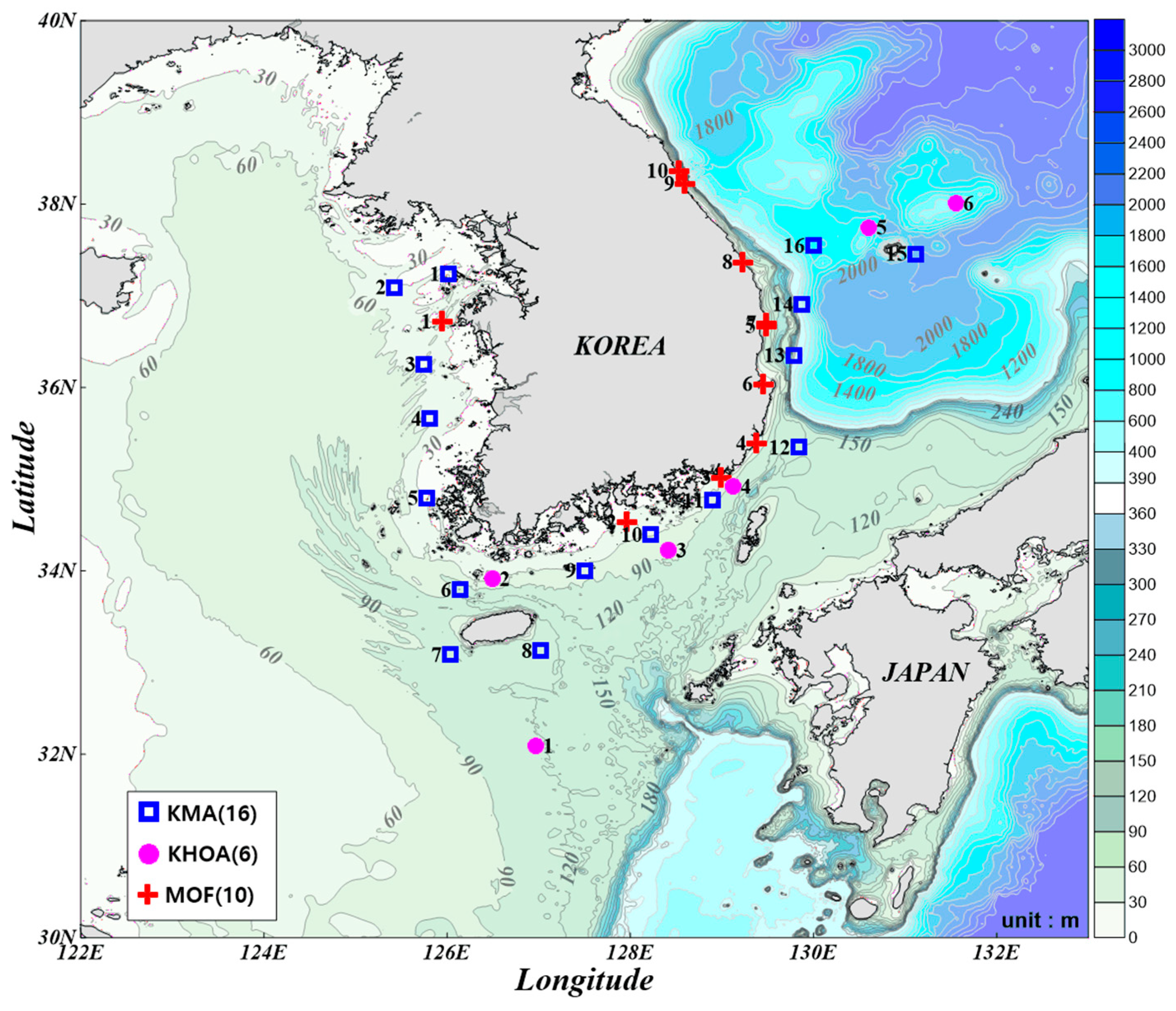
Article

Wave Energy in Korean Seas from 12-Year Wave Hindcasting

1
Geosystem Research Corporation, Department of Marine Forecast, 306, 172 LS-ro, Gunpo-si, Gyeonggi-do 15807, Korea
2
Coastal & Ocean Engineering Division, Korea Institute of Ocean Science and Technology, 385, Haeyang-ro, Yeongdo-gu, Busan 49111, Korea
*
Author to whom correspondence should be addressed.
J. Mar. Sci. Eng. 2020, 8(3), 161; https://doi.org/10.3390/jmse8030161
Submission received: 31 January 2020 / Revised: 24 February 2020 / Accepted: 26 February 2020 / Published: 2 March 2020
(This article belongs to the Special Issue Numerical Models in Coastal Hazards and Coastal Environment)

Abstract

:
In this study, a numerical simulation is performed to produce wave hindcasting data from 2007 to 2018 for the assessment of wave energy resources in the sea waters of Korea. The hindcasting data are obtained with a relatively fine spatial resolution of 1/20° covering 120–150 °E longitude and 22.4–47.6 °N latitude using the Simulating WAves Nearshore wave model (SWAN). Three different wind fields, those of the European Centre for Medium-Range Weather (ECMWF), National Centers for Environmental Prediction (NCEP), and Japan Meteorological Agency (JMA), are used for the numerical wave simulation. It is observed that the wind field dataset of JMA exhibits the best agreement with available field observation data. For this reason, the wave energy resources are evaluated based on the data hindcasted using the JMA wind field. It is found that the overall magnitudes of wave energy are larger in winter than in summer. The wave energy in August, however, is comparable to the mean wave energy during winter because of the influence of frequent high wave events caused by typhoons. The highest monthly average wave power around Yellow Sea, South Sea, East Sea, and Jeju Island are 13.3, 18.2, 13.7, and 40 kW/m, respectively.

1. Introduction

Recently, the regulations on the use of fossil fuels have been made more stringent because of worsening global warming and pollution. To resolve these problems, renewable energies derived from solar heat and tidal currents and waves are suggested as appropriate alternatives to fossil fuels. In this regard, various research works have been conducted in oceans because wide spaces are available, and the potential threat to human lives is lower than when these studies are conducted on land. For the successful production of these renewable energies in oceans, however, it is necessary to understand the capacity of available power before the infrastructures are built; thus, advanced thorough investigations are crucial. For example, in the case of wave power generation, a precise comprehension of the distributions and variation patterns of wave energy and other wave characteristics in a region of interest is imperative. This is difficult to achieve, however, because of the high variability and dispersion of wave fields over time and space. To determine wave characteristics at a specific location, observational data must be gathered at different points in the area over sufficiently long periods (at least 10 years). In most ocean areas, however, such data are not available. An alternative approach to understand wave characteristics in specific regions is hindcasting. This technique employs wave models by which previous wave conditions have been represented and improved through comparisons with observational data.
Previous studies on hindcast modeling for regional wave conditions have been reported. Bernardino et al. evaluated wave energy resources in the Cape Verde Islands in the Atlantic Ocean west of South Africa for 10 years (2004–2013) [1]. The Simulating WAves Nearshore (SWAN) [2] wave model was used, and the European Centre for Medium-Range Weather Forecasts (ECMWF) wind field was employed for wave forcing. The ERA-Interim (ECMWF reanalysis) dataset, which is a global atmospheric reanalysis from 1979 to 2019, was utilized with a 1° spatial resolution and a 6-h temporal resolution. In the Black Sea, the wave energy distribution over a 30-year period (1987–2016) was estimated using SWAN [3]. In this study, the U.S. NCEP–CFSR (National Centers for Environmental Prediction–Climate Forecast System Reanalysis) wind data are compared with ERA-Interim data. The NCEP–CFSR winds are finally applied to the wave model because of their better performance. Wave energy distributions have also been hindcasted using SWAN in the Persian Gulf [4], coastal regions of Portugal [5], and Iroise coasts of France [6]. The analyses in these studies are similar except for differences in the applied wind fields and hindcast durations. In the Persian Gulf, ECMWF ERA-40 data with a 0.2° resolution were used for 25 years from 1984 to 2005. In Portugal, ERA-Interim data with a 0.75° resolution were employed for 15 years from 2000 to 2014. In Iroise, France, ALADIN (Aire Limitée, Adaptation dynamique, Développement InterNational, Météo-France) [7], with a 10-km special resolution and 3-h time interval wind data, was employed for eight years from 2004 to 2011. In China, the wave energy field was hindcasted for 20 years from 1996 to 2015 [8]. In this study, CCMPV2.0 (Cross-Calibrated Multi-Platform Version 2.0) wind data [9] with a 0.25° resolution are utilized to calculate wave energy distributions in 17 regions, which are classified according to their distance from the coast.
The foregoing studies employed the SWAN wave model for hindcasting, but other similar research utilized different wave models. For example, Kim et al. evaluated the wave energy fields in the seas around the Korean Peninsula for 25 years from 1979 to 2003 [10]. In their study, various models were used at different periods according to wave conditions. Under extreme wave conditions, the wave prediction model (WAM) [11] was employed. Under normal wave conditions, the hybrid parametrical wave prediction model (HYPA) [12] was applied because of its shorter running time. The use of WAM and HYPA in this previous research, which was performed a decade ago, has motivated the conduct of the present study. Although SWAN has been used in most previous studies related to regional wave hindcasting, it has not been employed in the seas around the Korean Peninsula. The use of SWAN for hindcasting in this region is accordingly proposed in this paper. Another main objective of this study is to evaluate the wind fields used for wave forcing. According to previous studies, hindcasting accuracy depends on wind field selection. In the research of Kim et al. [10], only ECMWF data were used. In the present study, the performances of three different sets of wind data are tested through comparisons with updated observation data from the Wave Information Network of Korea (WINK, http://wink.kiost.ac.kr) system [13] to select the most suitable wind field for wave hindcasting. Additionally, although only the wave energy was previously evaluated in [10], the distributions of other wave parameters, such as wave height, period, and direction, are calculated in this study to increase the quantity of available data for researchers and other potential users.

2. Wind and Wave Data

2.1. Wind Data

Three wind products using the three wind datasets of the ECMWF, NCEP, and JMA are evaluated for wave hindcasting. The ECMWF and NCEP datasets are global products, whereas the JMA (Japan Meteorological Agency) dataset is a regional product for East Asia. The spatial resolutions of ECMWF, NCEP, and JMA are 0.125°, 0.205°, and 0.0625°, respectively. The time interval of ECMWF is 6 h, and that of NCEP and JMA is 1 h; wind product details are listed in Table 1.

2.2. Wave Data

In this study, the data employed for model evaluation are obtained from WINK because this system provides quality-controlled observational wave data from 32 stations (16, 6, and 10 stations are monitored by Korea Meteorological Administration (KMA), Korea Hydrographic and Oceanographic Agency (KHOA), and Ministry of Oceans and Fisheries (MOF), respectively). The locations of these stations and other salient details are shown and listed in Figure 1 and Table 2, respectively.

3. Numerical Model

3.1. Theoretical Formulations

The evolution of the action density N(E/σ, where E is the wave energy density distributed over intrinsic frequencies (σ) and propagation directions (θ)) is governed by the action balance equation.
N t + x , y [ ( C g + U ) N ] + σ ( C σ N ) + θ ( C θ N ) = S t o t σ
The quantities Cσ and Cθ are the propagation velocities in spectral space (σ, θ). The right-hand side contains Stot, which is the source/sink term that represents all physical processes which generate, dissipate, or redistribute wave energy.
S t o t = S i n + S n l 3 + S w c + S b o t + S b r k
These terms denote, respectively, wave growth by the wind, nonlinear transfer of wave energy through three-wave interactions [14] and wave decay due to whitecapping, bottom friction and depth-induced wave breaking. The energy transfer from wind to waves (Sin) and wave energy dissipation caused by whitecapping (Swc) are approached with the saturation-based model of Westhuysen [15] combined with the wind input formulation proposed by Yan [16]. The energy dissipation by bottom friction (Sbot) is computed according to the formulation developed by Madsen et al. [17]. The energy dissipation due to wave breaking (Sbrk) according to Battjes and Janssen [18].

3.2. Model Setup

In this study, the SWAN model version 40.91 is employed. The model has an orthogonal grid with a spatial resolution of 0.05° and covers 120°–150 °E longitude and 22.4°–47.6 °N latitude. The topographic data provided by KHOA are utilized for the model grid depth (Figure 2). The initial water level is set as the approximate highest high water level (AHHWL). By fixing the sea levels in all model runs, the change in water level caused by the tide is disregarded. The AHHWL, instead of the mean sea level, is used because tidal flats are widely generated on the western coast, and a significant portion of the sea has to be treated as land if the latter is applied. The two-dimensional wave spectrum used in the model consists of direction and frequency. The wave direction is divided into 48 segments, each of which is set at 7.5° wide. The frequency is divided into 20 bands within the (0.04–0.4)-Hz range. These 20 frequency bands may produce extremely wide bandwidths especially in long waves with lower frequency levels. To examine this, a sensitivity test with 40 bands is implemented. The model integration time usually increases with the frequency band. The computational cost can be reduced if the frequency bands are also reduced (provided that the results are stable). Figure 3 shows a comparison of wave parameters calculated in three different cases. In Case 1, 20 bands in the (0.04–0.4)-Hz frequency range are used. In Cases 2 and 3, 40 bands in the (0.04–0.4) and (0.02–0.4)-Hz frequency ranges are used and observed at the KMA-2 location, respectively. No distinct difference is found among the three cases, thus validating the use of 20 band levels to reduce computational cost.
In the model runs, only wind forcing is present, and no waves are set along the lateral boundaries, assuming that waves from the open seas do not enter the computational domain. For validation, the three wind fields of ECMWF, NCEP, and JMA are compared with the observational data measured in 2016; the setting details of the model are listed in Table 3. Other model conditions, such as ocean currents, are not considered in the experiments.

3.3. Comparison with Point Measurements

To evaluate the accuracy of wind datasets, the verification of three wind fields of ECMWF, NCEP, and JMA is conducted. Observational wind data from 22 stations monitored by the KMA and KHOA are used for the evaluation. Considering the spatial resolution of the model (0.05° or ~5 km), data from the six stations monitored by the MOF are excluded because these stations are close to the coast (water depths, 15–36 m).
The evaluation is performed using the correlation coefficient ( R = i ( ( x i x ) × ( y i y ) ) / ( i ( ( x i x ) 2 × ( y i y ) 2 ) ) ), root mean square error ( RMSE = i ( x i y i ) 2 / n ), and bias ( B = y ¯ x ¯ ), where x and y are the observation and model values, respectively. The R values of NCEP, ECMWF, and JMA are 0.902, 0.913, and 0.928, respectively; the RMSE values are 0.398, 0.377, and 0.318, respectively. The B values of NCEP, ECMWF, and JMA are 0.189, 0.200, and 0.094, respectively. The JMA wind data are the most accurate compared with those of NCEP and ECMWF (Table 4). For the wave by wave height evaluation, the wave height is classified as <1, 1–2, 2–3, and >3 m. The JMA data perform best among all wave levels (Table 5). Figure 4 shows the time series of model data and observational data from Jeju-South station monitored by the KHOA. The scatter diagrams for the 22 stations are shown in Figure 5. Based on the foregoing, the JMA wind data are selected to investigate the wave energy characteristics in the seas of Korean.

4. Wave Energy Resource Characterization

4.1. Wave Energy Calculation Method

Wave energy, P , can be calculated by
P = ρ g 2 64 π T e 2 H s 2
where H s is a significant wave height; is the specific density of water; is the gravitational acceleration; T e is the average wave period indicating the energy period and is usually determined as 90% of the peak wave period in the SWAN model [4,10]. Parameters H s and T e are obtained from the wave model outputs.

4.2. Spatial Distribution of Wave Energy

In order to investigate the wave energy distribution in Korean seas, the wave energy average over a span of 12 years (2007–2018) and the yearly wave energy average are shown in Figure 6 and Figure 7, respectively. The wave energy averages in the Yellow Sea, Korea Strait, East Sea, and the vicinity of Jeju Island are 0.6–13.3, 3–9, 3–8, and 7–12 kW/m, respectively (Figure 6). The yearly wave energy average for 12 years shown in Figure 7 indicates that the wave energy exceeds 15 kW/m in the vicinity of Jeju Island. The high wave energy around Jeju Island appears related to the fact that more high waves occur in its vicinity than in other regions when typhoons occur in summer.

4.3. Inter-Annual Wave Energy Evolution

In order to examine the characteristic features of wave energy distribution, the monthly wave energies in four regions (Yellow Sea, South Sea, East Sea, and Jeju Island vicinity) are listed in Table 6 and Table 7; the distribution map is shown in Figure 8. The time series of monthly wave energy for 12 years is shown in Figure 9. Figure 10 shows the monthly wave energy over 12 years. Figure 9 and the list in Table 7 suggest that the monthly wave energy is highly variable. The Yellow Sea has high variabilities: 3.2–8.6, 0.7–5.0, and 1.9–10.9 kW/m in February, June, and August, respectively. In May, however, the wave energy is at a minimum (0.6–2.5 kW/m) and with low variability. The wave energies in the Yellow Sea, South Sea, East Sea, and Jeju Island vicinity are 0.6–13.3, 1.1–18.2, 0.7–13.7, and 1.6–40 kW/m, respectively, suggesting high monthly variations. Generally, the wave energy reaches the maximum value and variability in winter and the minimum in summer (except for August). The high variability in August compared with the other months is possibly the effect of typhoons.
The results in Table 7 and Figure 9 represent the average wave energy in each region. If the wave energy average of the entire area is calculated, however, the result will not be relevant for wave energy exploitation because various depths are encountered. Figure 11 and the list in Table 8 are, therefore, included to compare the time series of wave energy computed at two selected locations in each region. The wave energy increases with the distance from the shore, except for the Yellow Sea, where the discrepancies among different locations are smaller than in other regions. In general, the magnitude of wave energy in the Yellow Sea, South Sea, and East Sea are similar, and the temporal variation is not significant. The wave energy in Jeju Island, however, is approximately two times greater than those in other regions; the magnitude is greatest in summer.

4.4. Seasonal Evolution of Wave Energy

In order to investigate the seasonal variation of wave energy, the monthly averaged wave energy over 12 years from 2007 to 2018 is used, as shown in Figure 12. Figure 13 shows the monthly averaged wave energy in February and August in 2007, 2012, and 2018. As shown in Figure 11, the wave energy is generally high in December and January and low in May and June. The lower energy during summer (except for August when typhoons and tropical storms cross the region) gradually increases with time and again peaks in December. The wave energy variability in the South Sea shown in Figure 13 is influenced by the occurrence of typhoons.

4.5. Wave Height, Period, and Direction

In Section 4.3, the analyzed data are presented in terms of wave energy distribution because the study aims to provide information for designing the wave power generation in the regions around the Korean Peninsula. In this section, additional hindcast data on other wave parameters, such as height, period, and direction, are described. Figure 14 and Figure 15 show the distributions of monthly mean wave height and period, respectively. The wave height distribution is similar to that of wave energy because it significantly increases in winter from December to February in all four regions. In December, the monthly mean wave heights increase to as high as 2 m in the East Sea and Jeju Island. The wave height decreases after winter and reaches the minimum in May. In August, however, the wave height near Jeju Island increases to ~1.5 m probably because of tropical storms that occasionally cross this region. On the other hand, the monthly variation in wave period is less significant because the spatial–temporal variations are not as distinct as the changes in wave height. The pattern, nevertheless, is generally similar to that of wave height because it increases in December, January, and February; in August, a significant increase in wave period is also observed near Jeju Island.
To understand the wave propagation directions, the rose diagrams of wave height and direction at eight selected locations in the four regions are presented in Figure 16. The wave direction exhibits distinct differences among the regions. In Jeju Island and the Yellow Sea, the waves generally approach the shore from the northwest. On the other hand, in the East and South Seas, they approach from the northeast. These patterns indicate that the waves developed in the Yellow Sea generally approach the coast from the northwest, whereas those generated in the East Sea approach from the northeast. It should be noted that the wave directions at P3 and P7 are clearly distinguishable although the distance between these two locations is only ~50 km.

4.6. Extreme Storm Events

In this section, the investigation of model performance under extreme wave conditions is presented. The Korean Peninsula is influenced by tropical storms because some of the typhoons that develop southwest of the North Pacific Ocean cross the East China Sea and East Sea. Table 9 lists the typhoons that influenced the Korean Peninsula from 2007 to 2018. The listed values were estimated at the time when these tropical cyclones passed over 30 °N latitude. During the 2007–2018 period, 23 typhoons were observed; six of these (NARI (2007), BOLAVEN (2012), SANBA (2012), DANAS (2013), GONI (2015), CHABA (2016)) were in the strongest intensity category because their maximum wind speeds exceeded 44 m/s. The storms that affected the Korean Peninsula exhibited high variance over the years because no typhoons were observed in 2008 and 2009; however, in 2012, five typhoons were monitored. Figure 17 shows the paths of these 23 typhoons. All the storms that moved to the west below 30 °N latitude passed over the East China Sea. Some of them, thereafter, changed directions toward the east and crossed the East Sea, thus impacting the southern and eastern coasts of the Korean Peninsula. The other storms continued to the north and passed through the Yellow Sea, thereby affecting the west coast.
In running the models for hindcasting, the impact of these typhoons is evaluated by means of the wind fields. In calculating the wave parameters and energy, however, it is found that the contributions of storms are indistinct.
The model performances using the wind fields during some of the tropical storms are compared. It is found that the outcomes of JMA best agree with observational data. In Figure 18, the model performance comparisons during Typhoons GONI (2015) and CHABA (2016) are provided for additional information.

5. Discussion

In this study, the SWAN wave model is employed for hindcasting. In reality, other wave models, such as WAM (wave model), can be used for similar purposes. For example, Kim et al. [10] used the HYPA and WAM for hindcasting in the seas around the Korean Peninsula. Their research motivated the present study. The SWAN model has been widely employed in hindcasting in other oceans and seas [1,3,4,6,7,8,9] but not in the seas around the Korean Peninsula. Apparently, it would be advantageous to use SWAN for hindcasting around this area. It should be noted, however, that the present study aims to determine the wind fields that are most appropriate for wave hindcasting in specific regions around the peninsula. Kim et al. [10] only utilized the ECMWF data for wind field hindcasting. It is, therefore, necessary to examine whether these data are indeed the best choice for wind field hindcasting or a better alternative dataset is available.
The results show that the JMA data better agree with measurements. Moreover, the hindcast model in the present study employs a finer resolution compared with that in Kim et al. [10]—the horizontal grid size in the latter is 1/6°, whereas 1/20° is employed in the experiments of the present study. A finer resolution is typically regarded as indicating that derived results are more accurate; consequently, the model outcomes may be deemed more credible by readers and potential users of published data. Although sensitivity tests among various hindcast models have not been performed in this study, these would have yielded valuable outcomes as well. The conduct of these tests is thus proposed in future studies. Among the deficiencies of the present research is the absence of lateral boundary conditions for the model and the assumption that no waves enter the computational domain simply because there is a dearth of information. In the low-frequency bands, however, long waves could propagate over extended distances and possibly affect wave conditions and distributions in the regions considered in this study. This aspect, therefore, also requires thorough consideration in future experiments.

6. Conclusions

It is advantageous to use wave data observed over a period of at least 10 years to determine the wave power generation in a particular location. In reality, however, it is difficult to continuously measure wave data over a 10-year period in the ocean; hence, such field datasets are rarely obtained. Alternatively, wave information could be obtained from hindcast simulations using wave models. Based on the foregoing, the present study is designed to derive information on the distributions of wave energy and other relevant parameters in the four regions around the Korean Peninsula—Yellow Sea, South Sea, East Sea, and Jeju Island.
Before hindcasting is conducted, the reproducibility of wave fields between the wind products of ECMWF, NCEP, and JMA is evaluated through comparisons with observational data from 21 stations. The results show that the differences among the wind fields are statistically significant. Furthermore, because the JMA wind field exhibits the highest correlation coefficient and the lowest root mean square and bias error, it is considered the best dataset among the three. Based on these results, the JMA wind data are selected for the conduct wave hindcasting using the SWAN model over a 12-year period (2007–2018) to investigate the characteristic patterns of wave energy distributions in the four regions.
Among the four regions, it is found that the wave energy near Jeju Island is the highest then followed by that in the South Sea; the lowest is observed in the Yellow Sea. The seasonal variability of wave energy is also observed to be high around Jeju Island. Its maximum is reached in December and January, and its minimum occurs in May. In August, the wave energy near Jeju Island sharply increases because of the occasional occurrence of typhoons that pass through this region. Around the island, the other wave parameters, such as wave height, period, and direction, also exhibit a pattern similar to that of wave energy. The wave height and period reach the maximum in December, January, and February and thereafter gradually decrease (except for August, when these parameters increase). The wave direction also exhibits severe spatial discrepancies because the waves in the Yellow Sea and near Jeju Island generally approach the shore from the northwest, whereas those in the South and East Seas approach from the northeast. The foregoing indicates that the waves in the coasts along the Korean Peninsula mainly develop in the northern parts of the Yellow Sea and East Sea.
The regions considered in the present study have been influenced by the occasional occurrence of typhoons. Accordingly, it is necessary to examine the performance of the hindcast model under extreme conditions. Through comparisons, it is confirmed that among the three wind fields, the JMA wind field dataset best agrees with observational data measured during major typhoons (such as GONI (2015) and CHABA (2016)). Although it is found that the energy generated by the waves in the seas around the Korean Peninsula (specifically near Jeju Island) may be sufficiently high for wave power generation, further investigations are necessary because the results of the present study only focused on determining the most appropriate wind field for hindcast simulations. Model validations through comparisons with additional observational data and other wave models are thus suggested for future investigations.

Author Contributions

Conceptualization, H.-S.E.; methodology, W.-M.J.; validation, J.-J.P. and S.-H.O.; formal analysis, H.-S.E. and W.-M.J.; investigation, J.-J.P. and S.-H.O.; data curation, J.-J.P.; writing—original draft preparation, H.-S.E., S.-H.O, and Y.S.C.; writing—review and editing, H.-S.E., W.-M.J., Y.S.C., S.-H.O., and J.-J.P. All authors have read and agreed to the published version of the manuscript.

Funding

This study was supported by Korea Institute of Ocean Science and Technology (project No. PE99832).

Acknowledgments

This research was supported by a grant (2018-MOIS31-008) from the Fundamental Technology Development Program for Extreme Disaster Response funded by the Ministry of Interior and Safety (MOIS, Korea).

Conflicts of Interest

The authors declare no conflicts of interest.

Abbreviations

AHHWLApproximation Highest High Water Level
ALADINAire Limitée, Adaptation dynamique, Développement InterNational
BBisa
CCMPV2.0Cross-Calibrated Multi-Platform Version 2.0
ECMWFThe European Centre for Medium-Range Weather Forecasts
ERA-InterimECMWF Reanalysis-Interim
ESEast Sea
HYPAHybrid PArametrical wave prediction model
JIJeju Island
JMAJapan Meteorological Agency
KHOAKorea Hydrographic and Oceanographic Agency
KMAKorea Meteorological Administration
KSKore Strait
MOFMinistry of Oceans and Fisheries
MSLMean Sea Level
NCEP–CFSRU.S. National Centre for Environmental Prediction
RCorrelation Coefficient
RMSERoot Mean Square Error
SWANSimulating WAves Nearshore
WAMWAve Prediction Model
WINKWave Information Network of Korea
YSYellow Sea

References

  1. Bernardino, M. Evaluation of the wave energy resources in the Cape Verde Islands. Renew. Energy 2017, 101, 316–326. [Google Scholar] [CrossRef]
  2. Booij, N. A third-generation wave model for coastal regions: 1. Model description and validation. J. Geophys. Res. 1999, 104, 7649–7666. [Google Scholar] [CrossRef] [Green Version]
  3. Lopez, M. The wave and wind power potential in the western Black Sea. Renew. Energy 2019, 139, 1146–1158. [Google Scholar]
  4. Kamranzad, B. Assessment of wave energy variation in the Persian Gulf. Ocean Eng. 2013, 70, 72–80. [Google Scholar] [CrossRef] [Green Version]
  5. Rusu, E. Study on the influence of the distance to shore for a wave energy farm operating in the central part of the Portuguese nearshore. Energy Convers. Manag. 2016, 114, 209–223. [Google Scholar] [CrossRef]
  6. Guillou, N.; Chapalain, G. Numerical modelling of nearshore wave energy resource in the Sea of Iroise. Renew. Energy 2015, 83, 942–953. [Google Scholar] [CrossRef] [Green Version]
  7. Benard, P. Aladin-nh/arome dynamical core; status and possible extension to IFS. In Proceedings of the ECMWF Seminar, Reading, UK, 6 September 2004; pp. 714–726. [Google Scholar]
  8. Yifan, L. Wave energy assessment in the China adjacent seas on the basis of a 20-year SWAN simulation with unstructured grids. Renew. Energy 2019, 136, 275–295. [Google Scholar]
  9. Atlas, R. A cross-calibrated, multiplatform ocean surface wind velocity product for meteorological and oceanographic applications. Bull. Am. Meteorol. Soc. 2011, 92, 157–174. [Google Scholar] [CrossRef]
  10. Kim, G.; Jeong, W.M.; Lee, K.S.; Jun, K.; Lee, M.E. Offshore and nearshore wave energy assessment around the Korean Peninsula. Energy 2011, 36, 1460–1469. [Google Scholar] [CrossRef]
  11. The WAMDI Group. The WAM model e, a third generation wave prediction model. J. Phys. Oceanogr. 1988, 18, 1775–1810. [Google Scholar] [CrossRef] [Green Version]
  12. Günter, H. A hybrid parametrical wave prediction model. J. Geophys. Res. 1979, 84, 5727–5738. [Google Scholar] [CrossRef]
  13. Ministry of Oceans and Fisheries (MOF). WINK System. Available online: http://wink.kiost.ac.kr (accessed on 2 March 2019).
  14. Eldeberky, Y. Nonlinear Transformation of Wave Spectra in the Nearshore Zone. Ph.D. Thesis, Department of Civil Engineering, Delft University of Technology, Delft, The Netherlands, 1996. [Google Scholar]
  15. van der Westhuysen, A.J. Advances in the Spectral Modelling of Wind Waves in the Nearshore. Ph.D. Thesis, Faculty of Civil Engineering, Delft University of Technology, Delft, The Netherlands, 2007. [Google Scholar]
  16. Yan, L. An Improved Wind Input Source Term for Third Generation Ocean Wave Modelling; Technical Report 87–88; Royal Netherlands Meteorological Institute (KNMI): De Bilt, The Netherlands, 1987. [Google Scholar]
  17. Madsen, O.S.; Poon, Y.K.; Graber, H.C. Spectral wave attenuation by bottom friction: Theory. In Proceedings of the 21st International Conference on Coastal Engineering, Sol-Malaga, Spain, 20–25 June 1988; ASCE: Reston, VA, USA, 1988; pp. 492–504. [Google Scholar]
  18. Battjes, J.; Janssen, J. Energy loss and set-up due to breaking of random waves. In Proceedings of the 16th International Conference on Coastal Engineering, Hamburg, Germany, 27 August–3 September 1978; pp. 569–587. [Google Scholar]
Figure 1. Locations of wave observation stations around Korean Peninsula provided by the Wave Information Network of Korea (WINK) system.
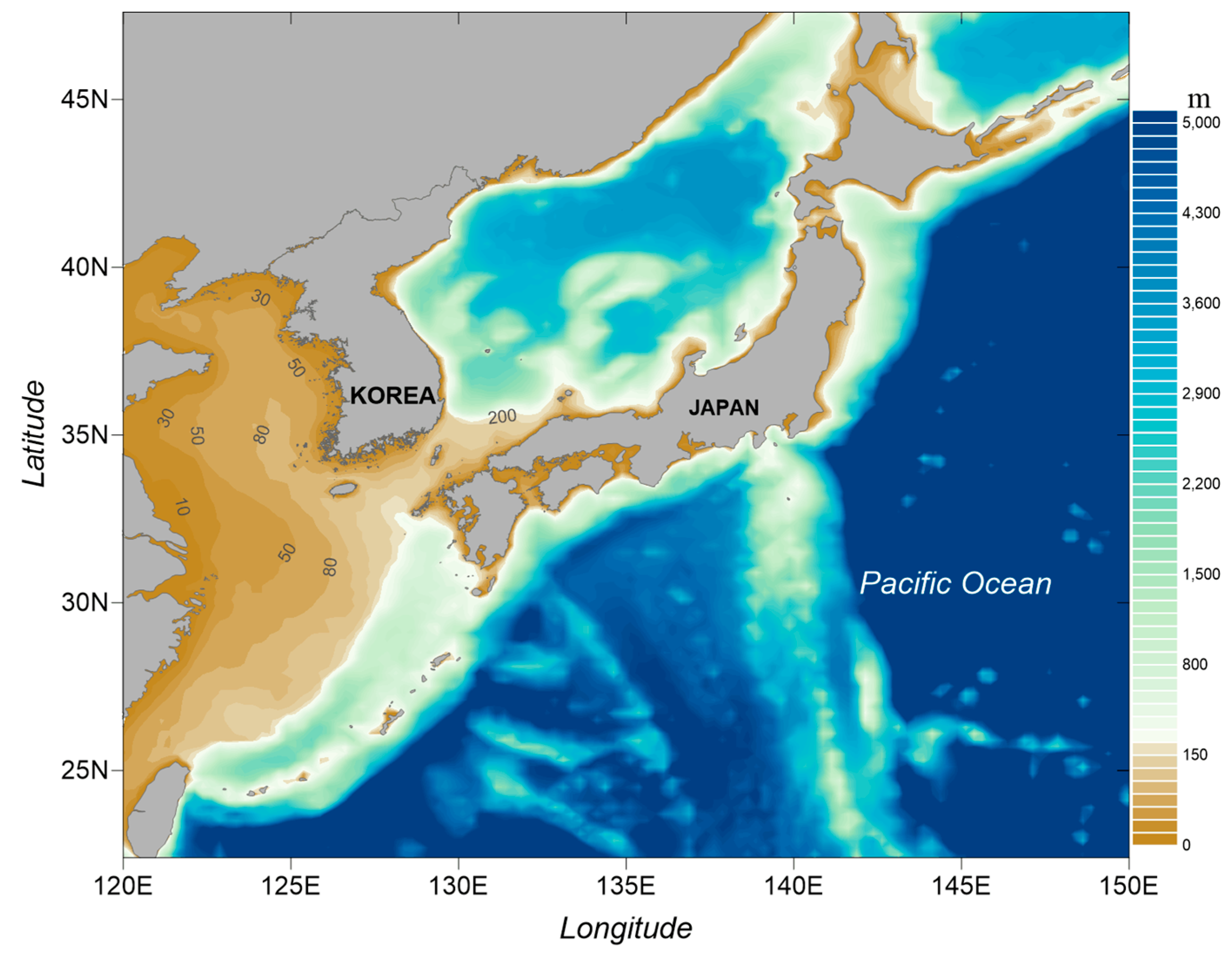
Jmse 08 00161 g001
Figure 2. Sea bottom bathymetry of geographical area simulated by the simulating waves nearshore (SWAN) model.
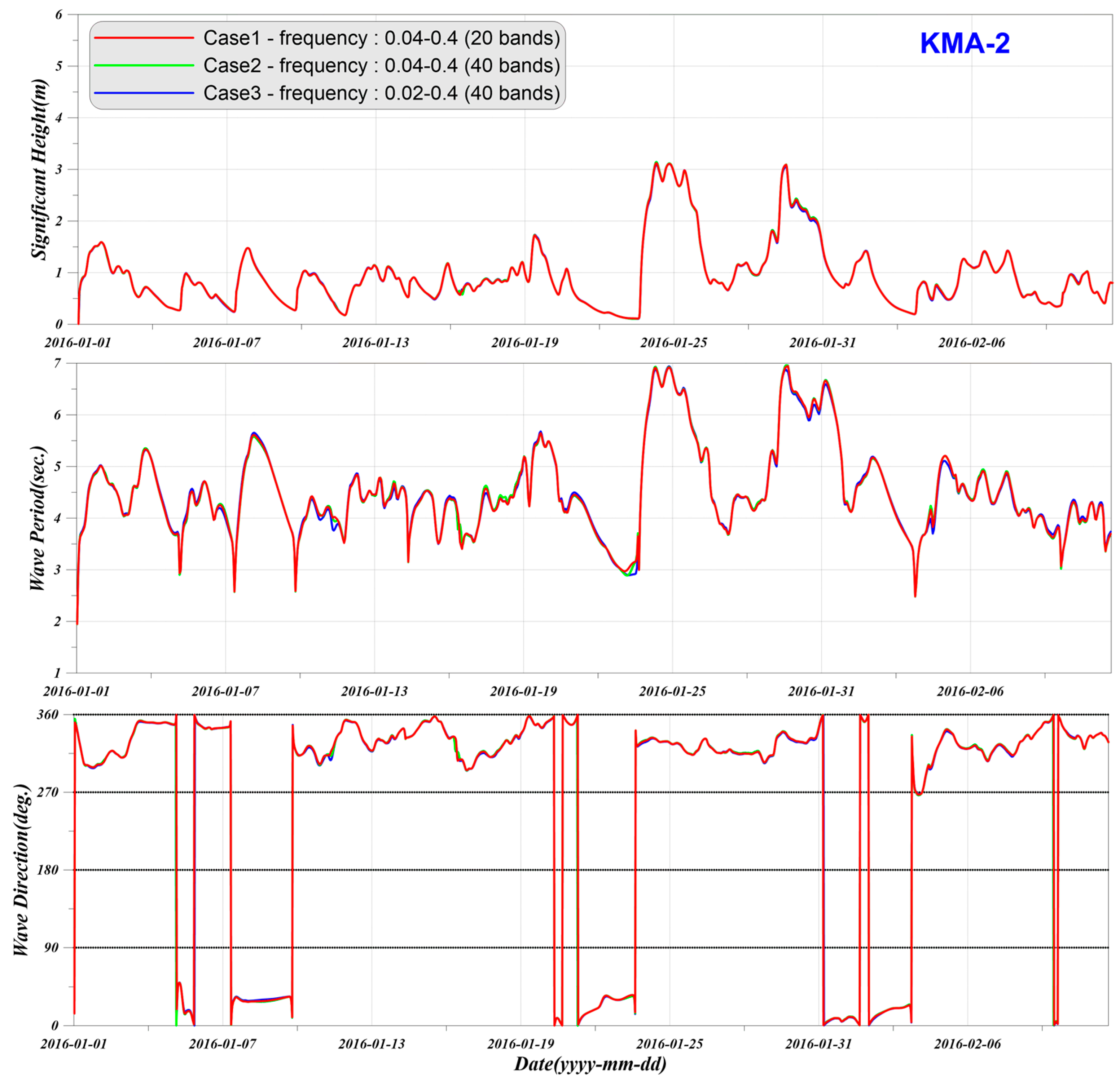
Jmse 08 00161 g002
Figure 3. Comparison of wave parameters (wave height, period, and direction) among the three different wave bands at KMA-2 location. Case 1: 20 bands in (0.04–0.4)-Hz frequency range; Case 2: 40 bands in (0.04–0.4)-Hz frequency range; Case 3: 40 bands in (0.02–0.4)-Hz frequency range.
Jmse 08 00161 g003
Figure 4. Measured and computed time series of significant wave heights at Korea Hydrographic and Oceanographic Agency (KHOA)-Jeju-South station in 2016.
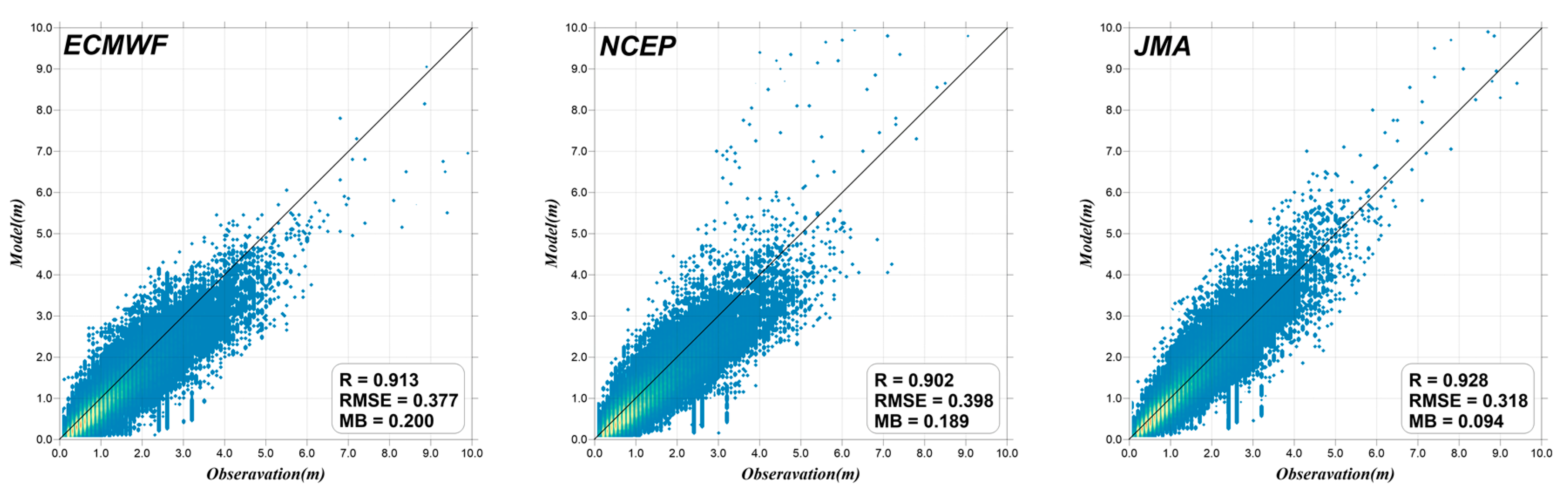
Jmse 08 00161 g004
Figure 5. Scatter diagrams of measured and hindcasted significant wave heights around the Korean Peninsula over 2007–2018.
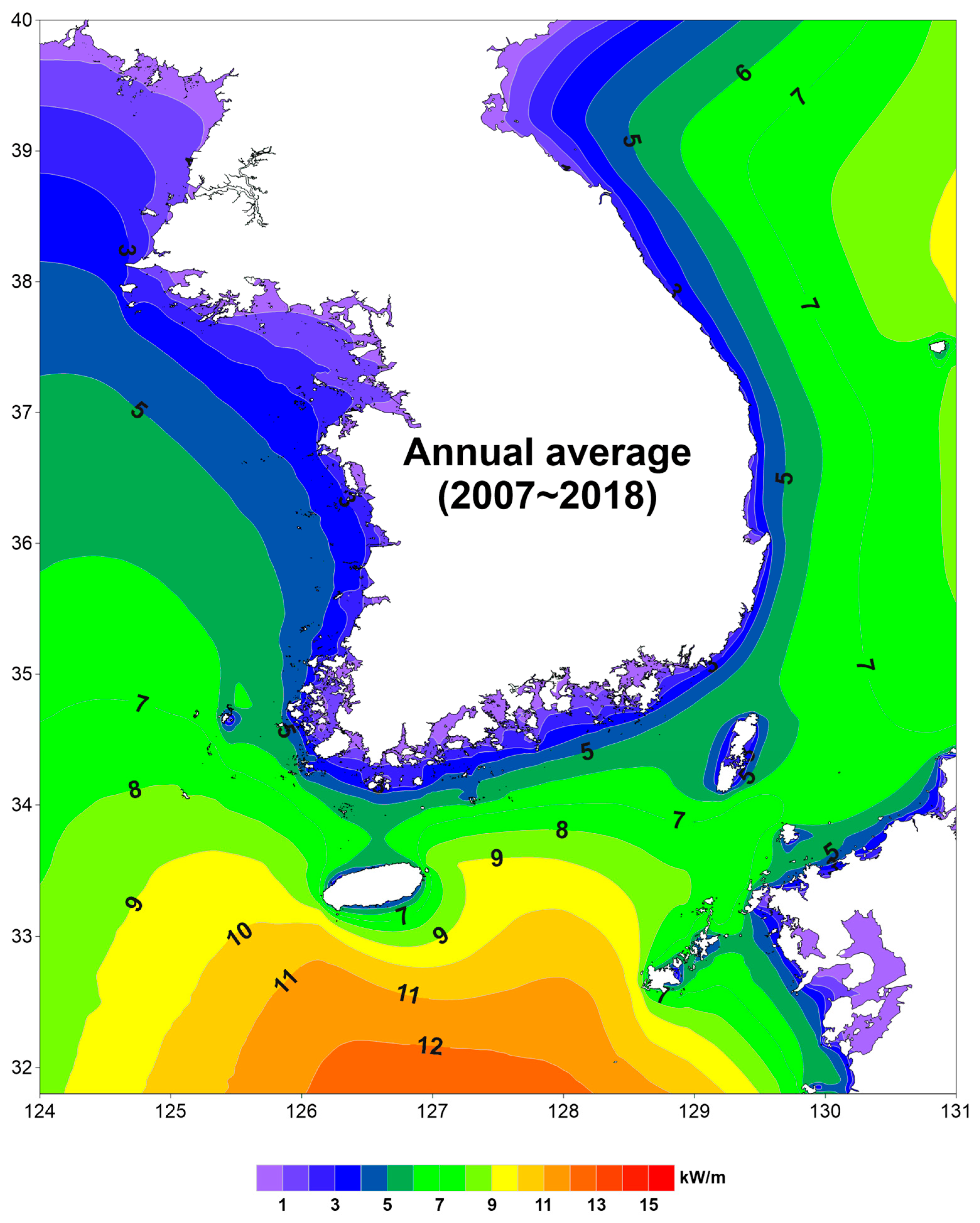
Jmse 08 00161 g005
Figure 6. Average wave energy over 12 years from 2007 to 2018.
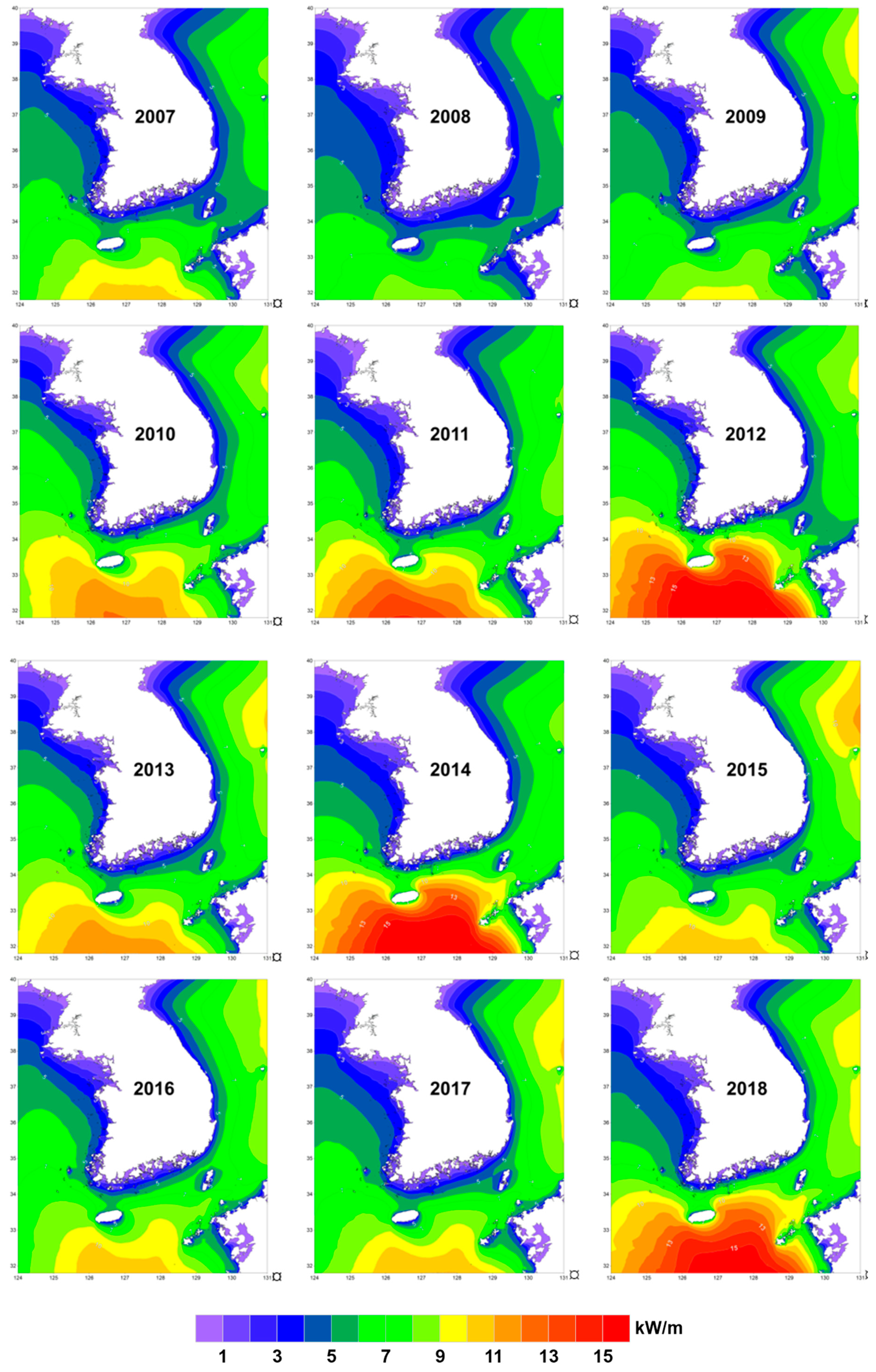
Jmse 08 00161 g006
Figure 7. Yearly wave power average around the Korean Peninsula over 2007–2018.
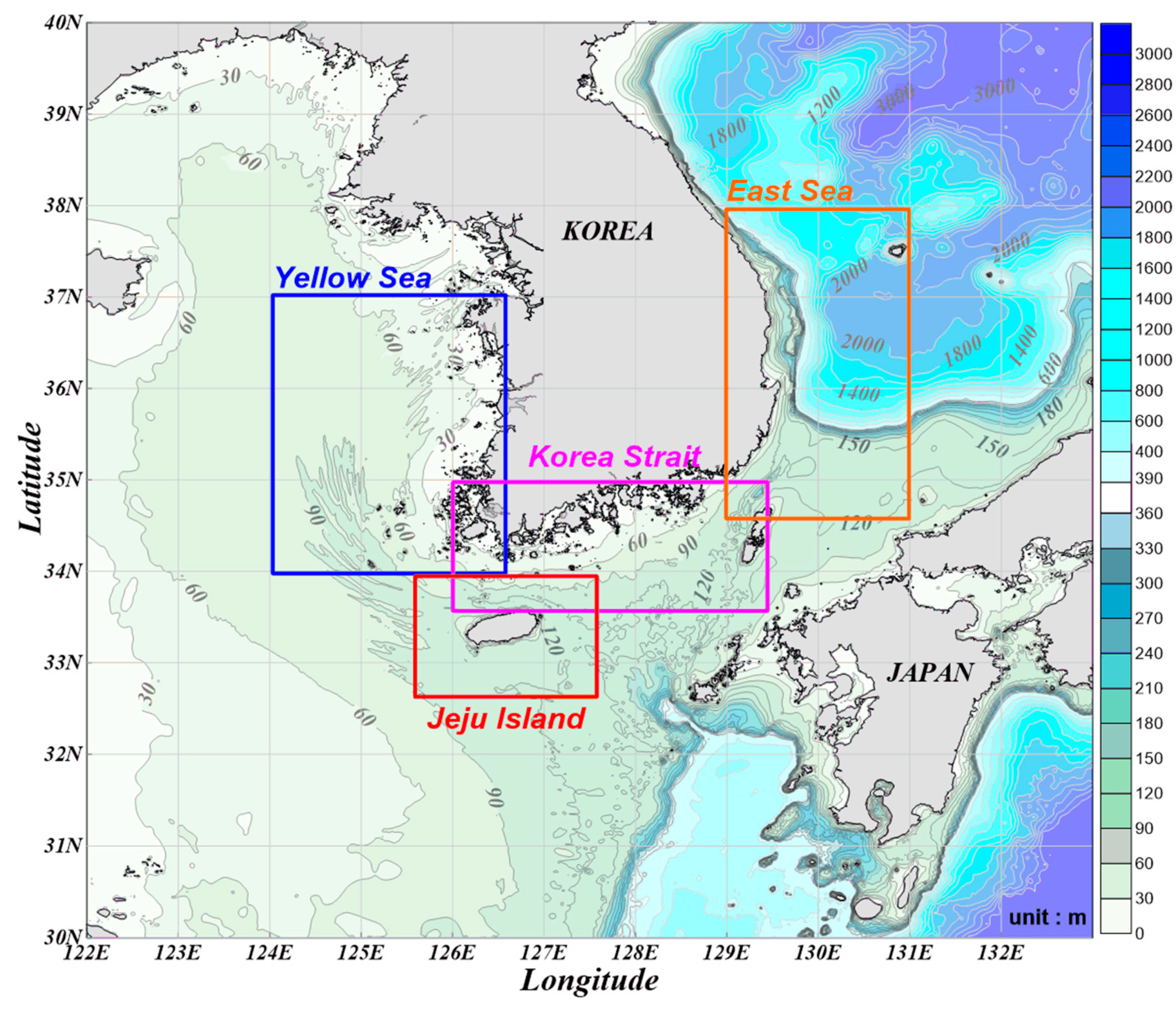
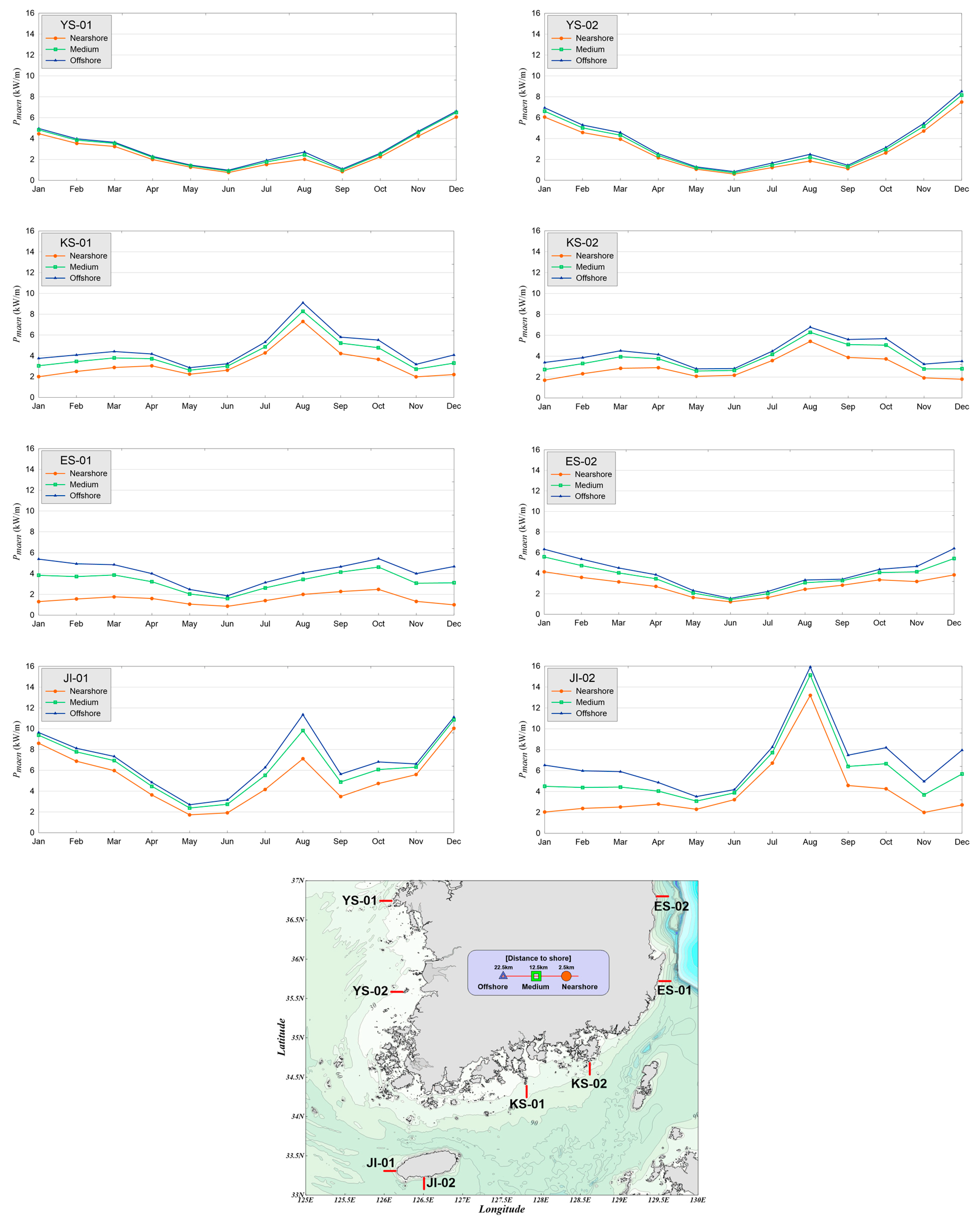
Jmse 08 00161 g007
Figure 8. Four selected regions for wave power calculation in the Yellow Sea, Korea Strait, East Sea, and Jeju Island.
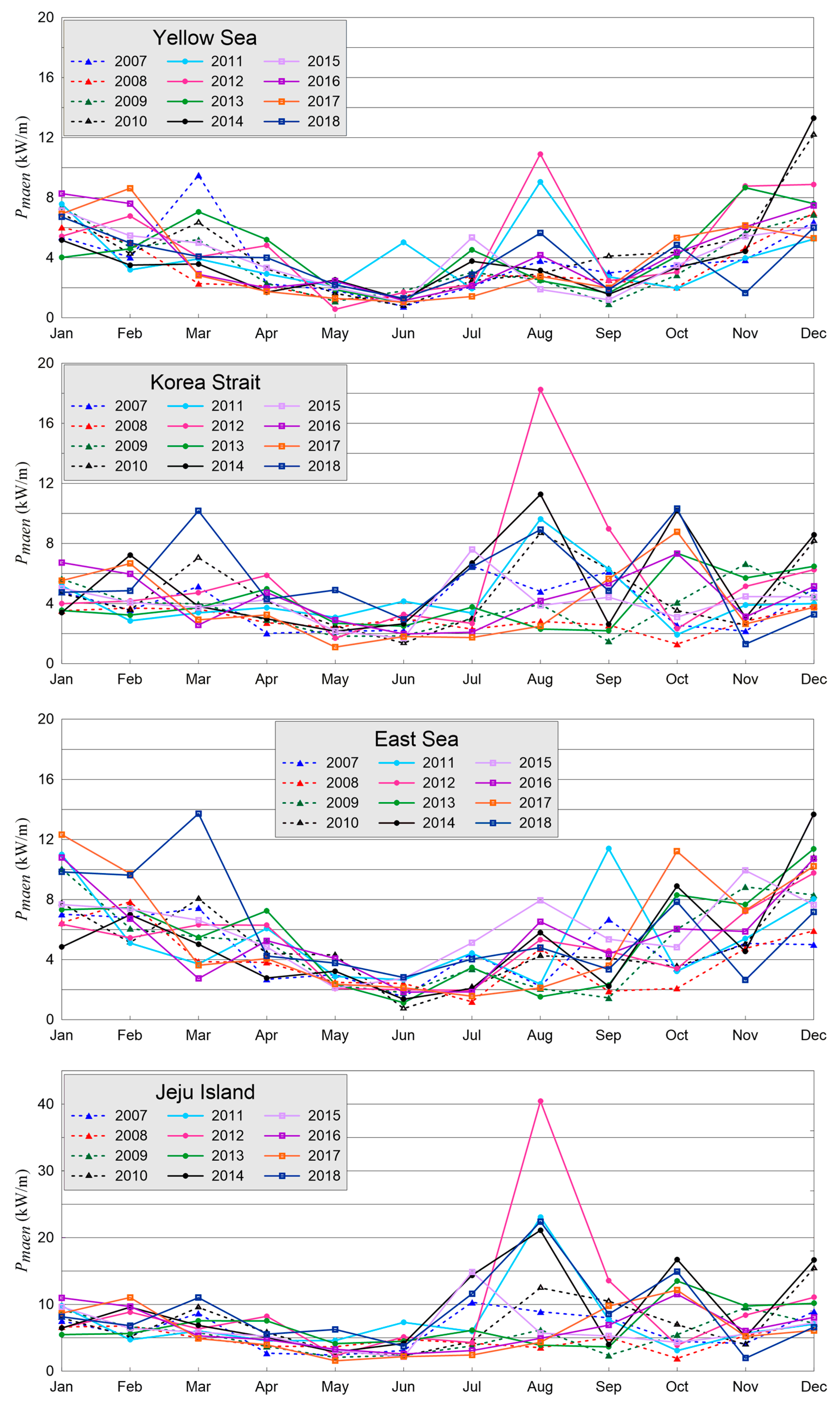
Jmse 08 00161 g008
Figure 9. Time series of monthly overall predicted wave power around the Korean Peninsula (Yellow Sea, Korea Strait, East Sea, Jeju Island) over 2007–2018. Note that the maximum value in the Y-axis for Jeju Island is 40.
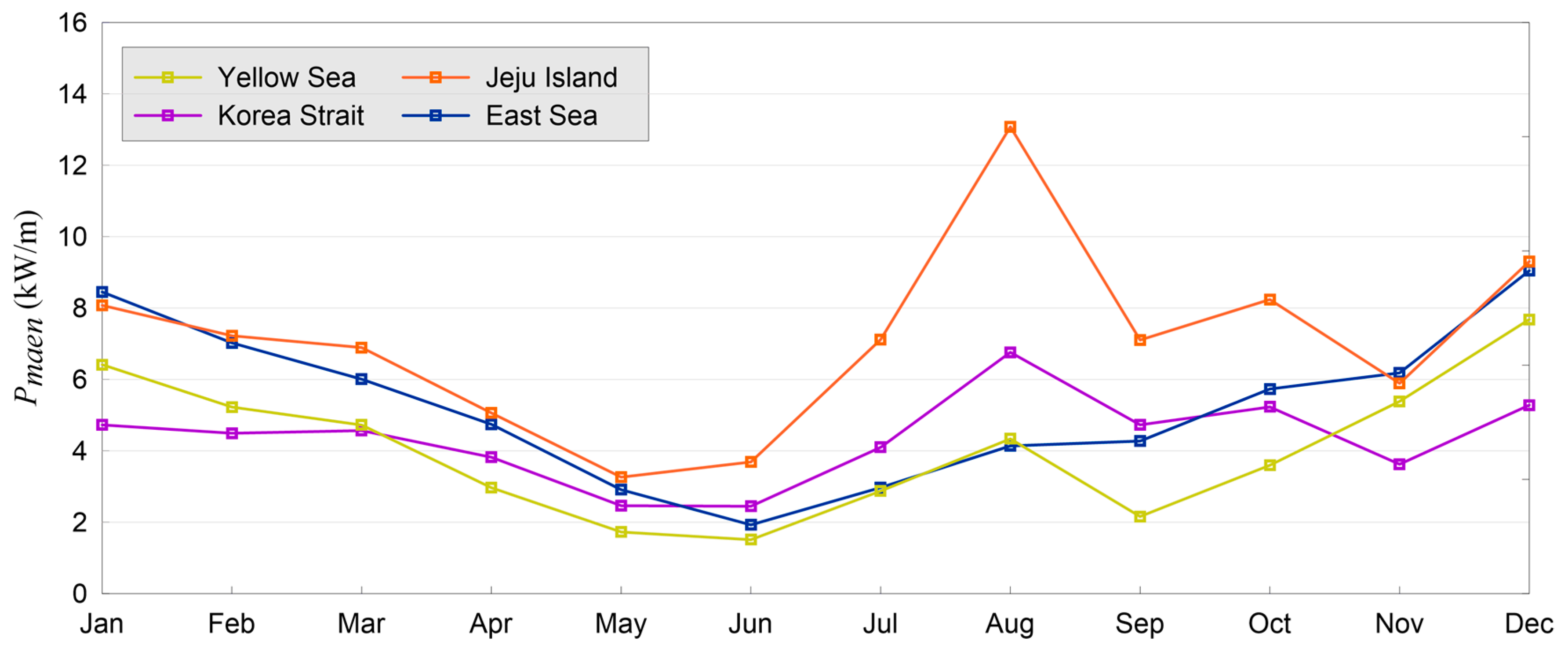
Jmse 08 00161 g009
Figure 10. Monthly wave power in the Yellow Sea, Korea Strait, East Sea, and Jeju Island averaged over 12 years from 2007 to 2018.
Jmse 08 00161 g010
Figure 11. Time series of monthly mean wave energy computed at two selected locations for each region over 2007–2018. The orange, green, and blue lines denote the locations where the energies are computed; their distances from the shore are 2.5 (nearshore), 12.5 (medium), and 22.5 km (offshore), respectively.
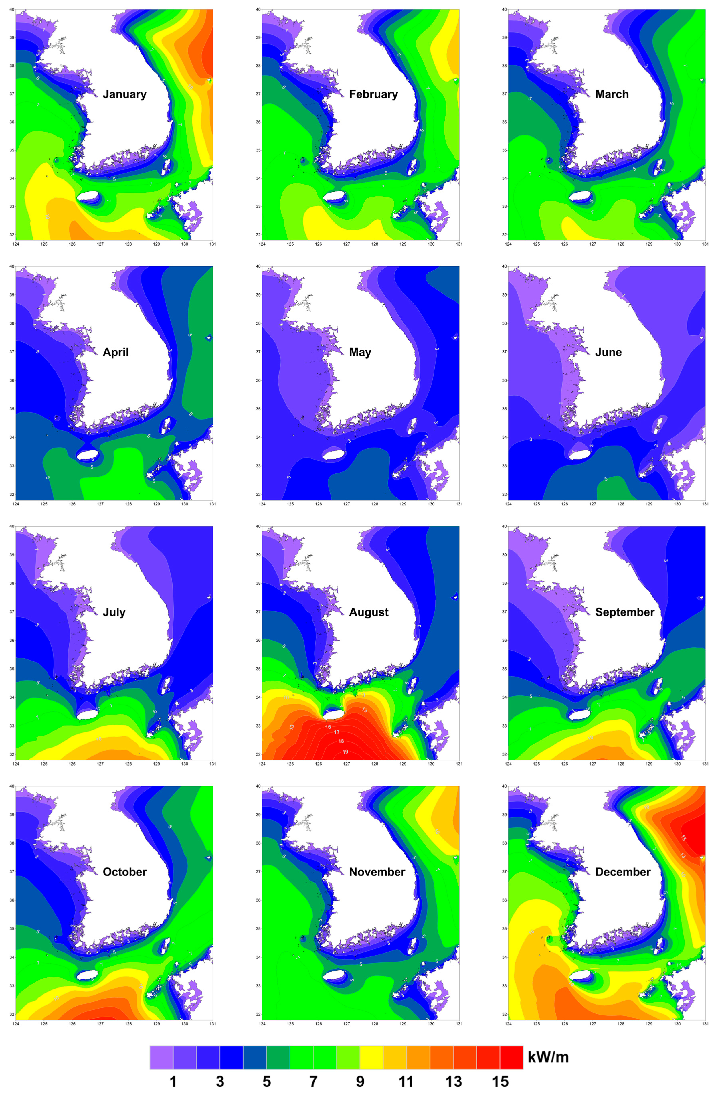
Jmse 08 00161 g011
Figure 12. Monthly wave power around the Korean Peninsula over 2007–2018.
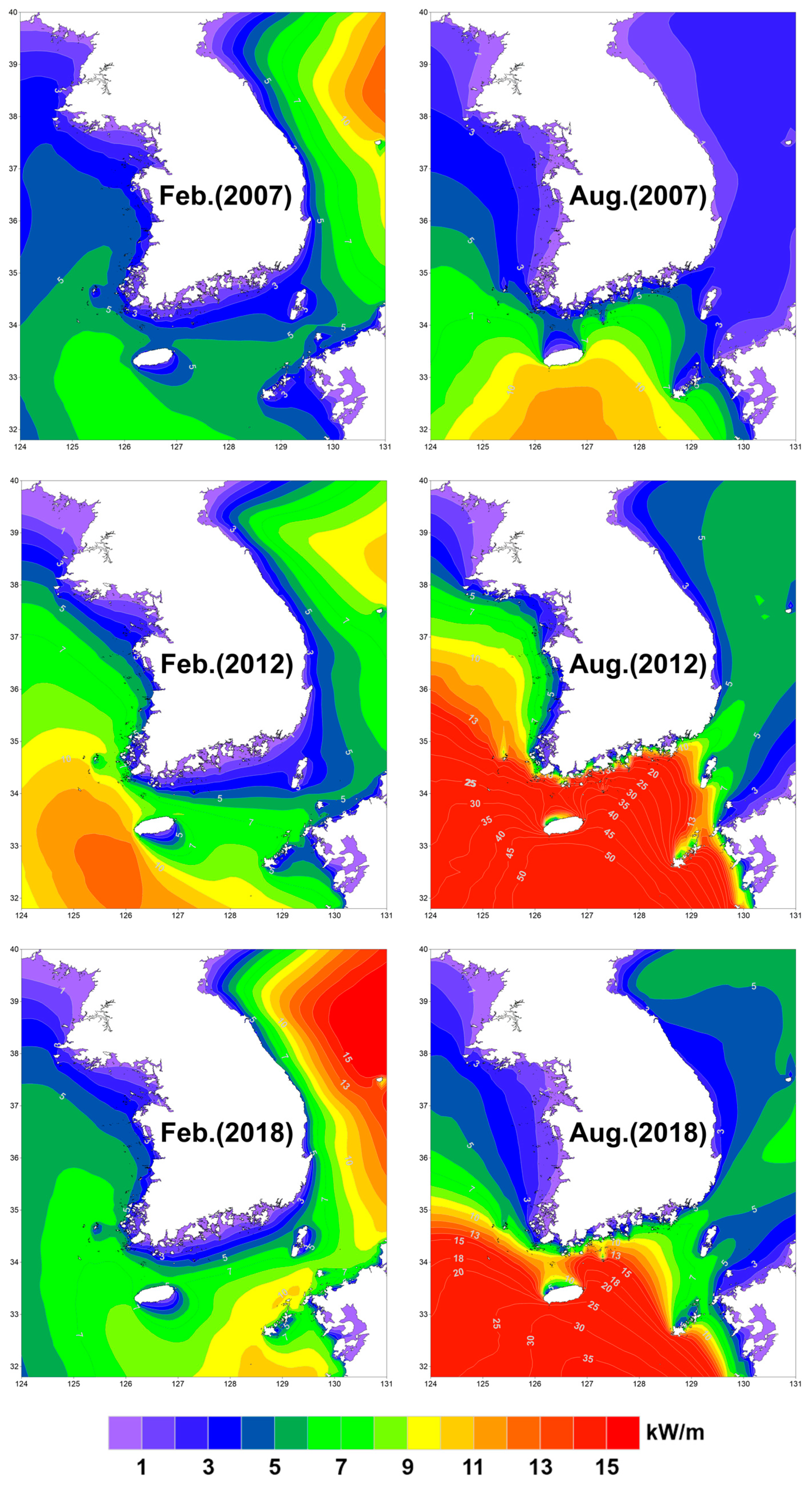
Jmse 08 00161 g012
Figure 13. Monthly averaged wave power of February and August around the Korean Peninsula in 2007, 2012, and 2018.
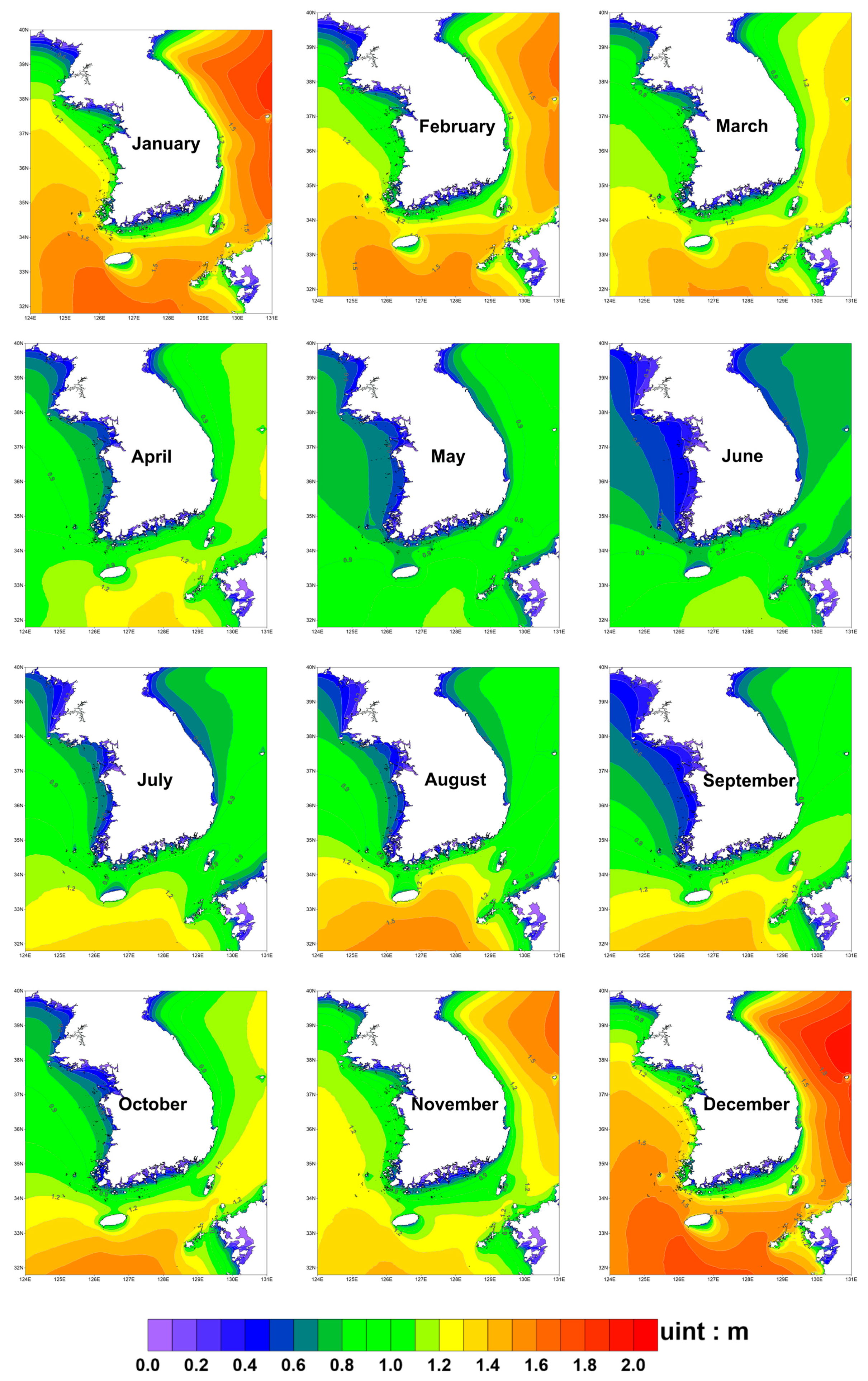
Jmse 08 00161 g013
Figure 14. Monthly averaged wave height around the Korean Peninsula over 2007–2018.
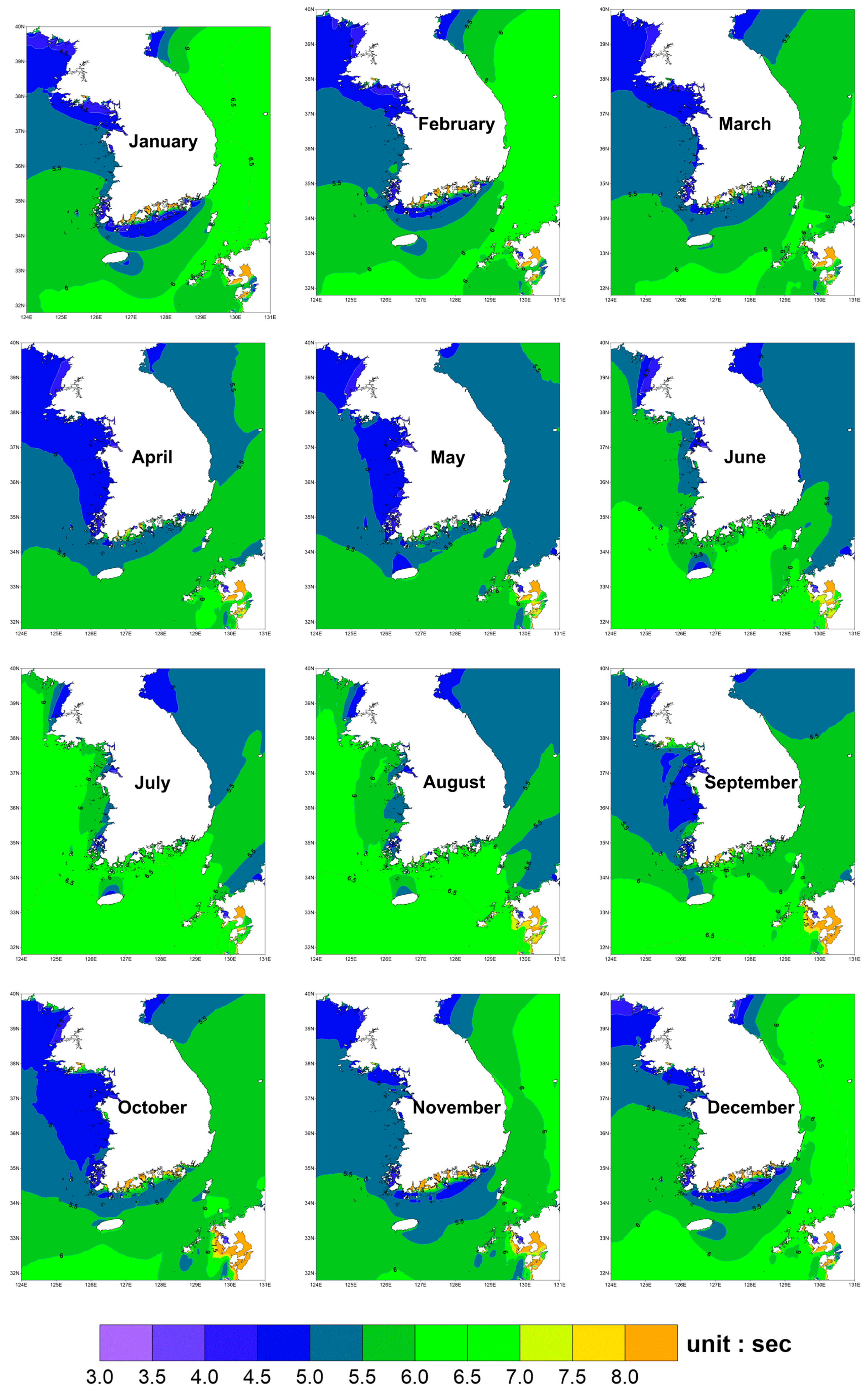
Jmse 08 00161 g014
Figure 15. Monthly averaged wave period around the Korean Peninsula over 2007–2018.
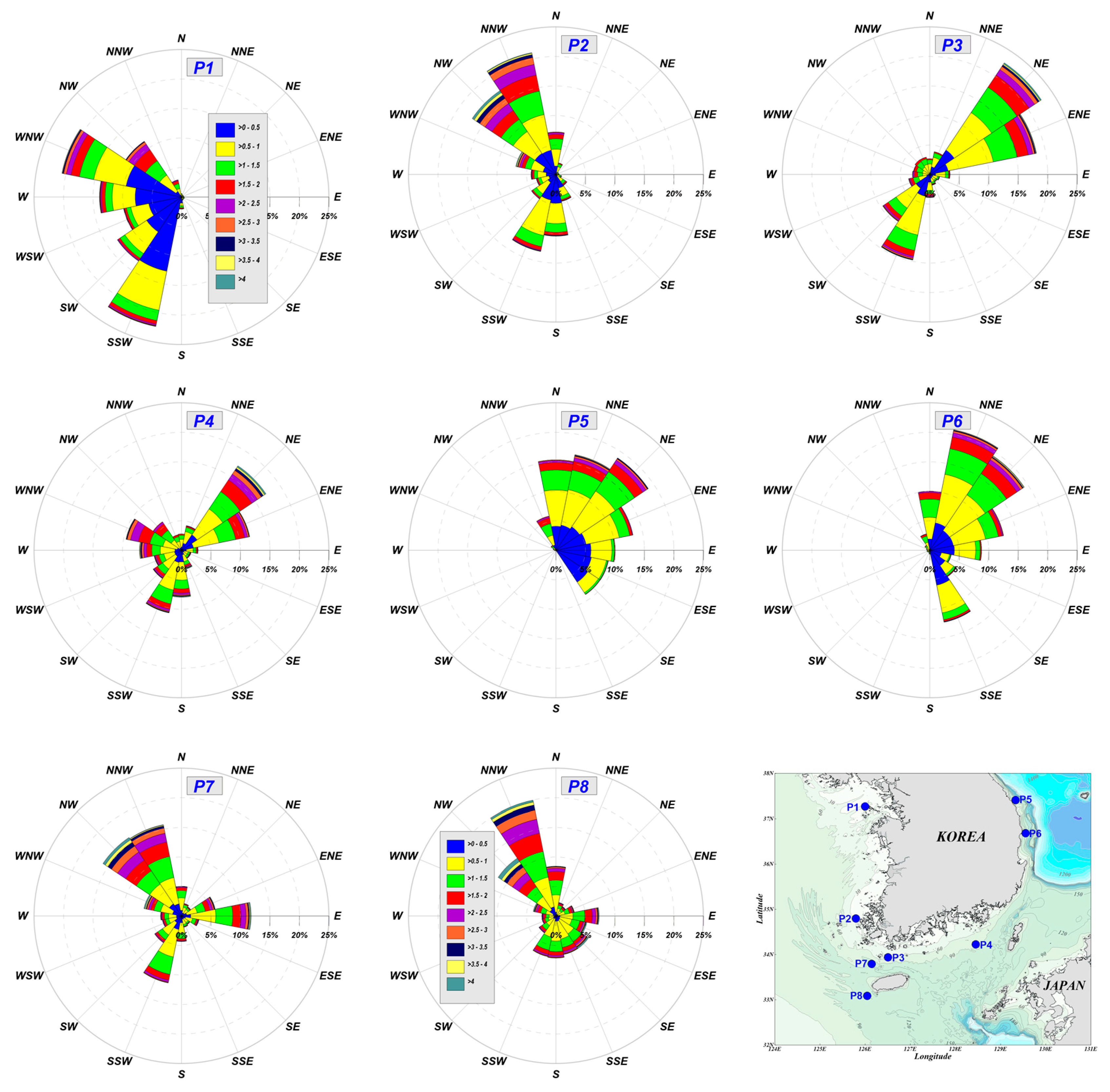
Jmse 08 00161 g015
Figure 16. Rose diagram of averaged wave height and direction at eight selected locations in four regions around the Korean Peninsula over 2007–2018.
Jmse 08 00161 g016
Figure 17. Paths of typhoons that affected the Korean Peninsula: (a) 2007–2013 and (b) 2014–2018.
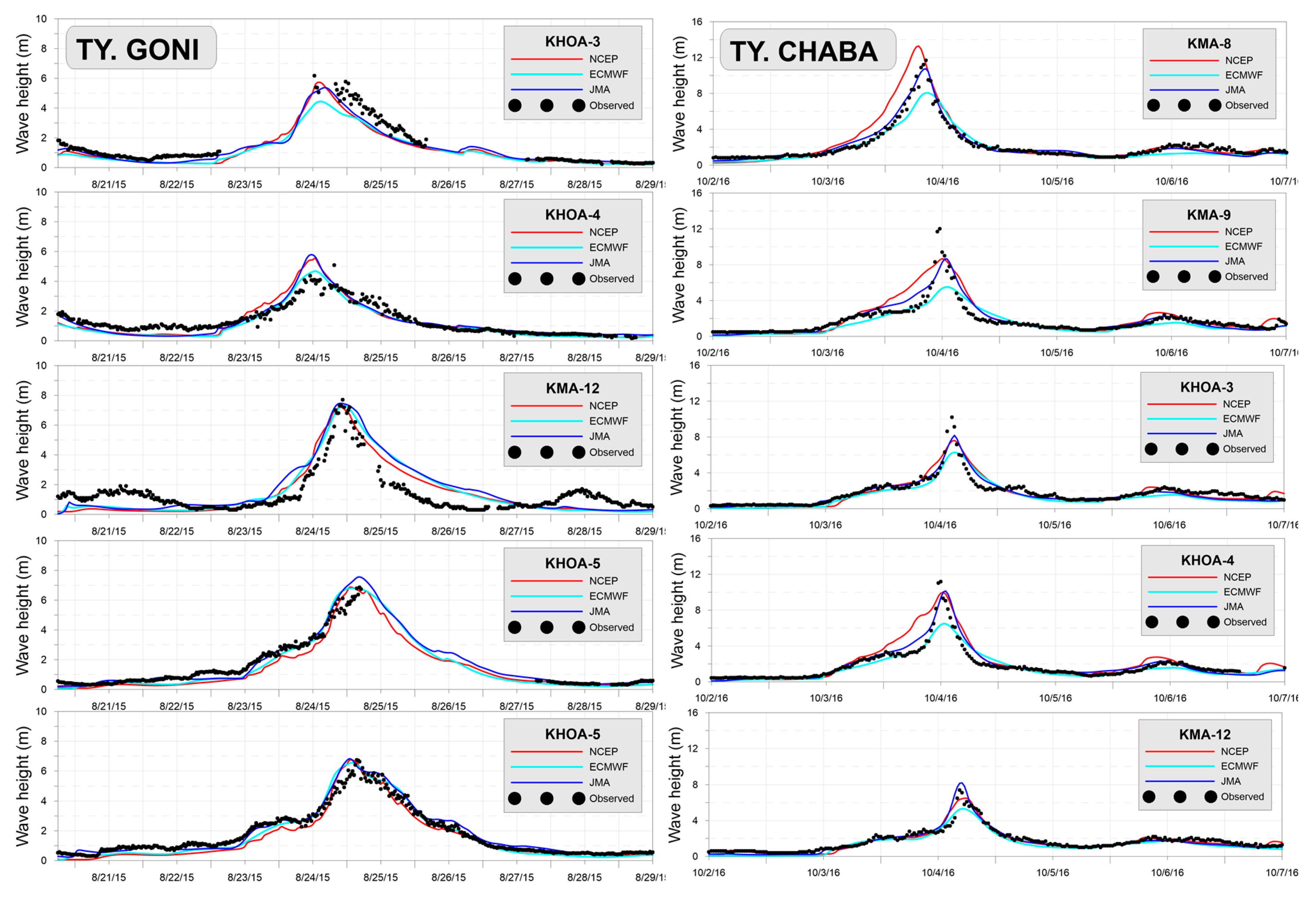
Jmse 08 00161 g017
Figure 18. Measured and computed time series of significant wave heights among the three wind fields during Typhoons GONI (2015) and CHABA (2016).
Jmse 08 00161 g018
Table 1. Summary of European Centre for Medium-Range Weather (ECMWF), National Centers for Environmental Prediction (NCEP), and Japan Meteorological Agency (JMA) wind data.
Wind DataSpatial ResolutionPeriodTime ResolutionArea
(°)(h)
ECMWFSet A1.1251979.01–1993.126Global
Set B1.1251994.04–2006.02
Set C0.252006.03–2012.01
Set D0.1252012.02–current
NCEPSet A0.3121979.01–2010.121Global
Set B0.205 × 0.2042011.01–current
JMA0.0625 × 0.0502006.03–current3120–150 °E, 22.4–47.6 °N
* Winds fields are based on U10, i.e., wind speed (m/s) at a height of 10 m above the sea surface.
Table 2. Summary of wave observation data provided by the WINK system.
NOSite NameObservation Start TimeObservation LocationWater Depth
KMA1Deokjeokdo1996.07.0137°14′9.96″N126°1′7.68″E37 m
2Incheon2015.12.2237°5′30.12″N125°25′44.04″E45 m
3Weyeondo2009.10.2136°15′0″N125°45′0″E58 m
4Buan2015.12.2235°39′30.96″N125°48′50.04″E59 m
5Chilbaldo1996.07.0134°47′35.88″N125°46′36.84″E36 m
6Chujado2014.01.1433°47′36.96″N126°8′27.96″E111 m
7Marado2008.11.1533°4′59.88″N126°1′59.88″E116 m
8Seogwipo2015.12.2233°7′41.16″N127°1′22.08″E115 m
9Geomundo1997.05.0134°0′5.04″N127°30′5.04″E81 m
10Tongyeong2015.12.2234°23′30.12″N128°13′30″E65 m
11Geojedo1998.05.0134°46′0.12″N128°54′0″E89 m
12Ulsan2015.12.2235°20′43.08″N129°50′29.04″E144 m
13Pohang2008.11.1536°21′0″N129°46′59.88″E372 m
14Uljin2015.12.0936°54′24.84″N129°52′27.84″E789 m
15Ulreungdo2011.12.2837°27′19.44″N131°6′51.84″E2123 m
16Donghae2001.04.0137°32′39.12″N130°0′0″E1520 m
KHOA1Jeju-South2012.11.1632°5′25″N126°57′57″E122 m
2Jeju Strait2012.11.1633°54′42″N126°29′32″E67 m
3South Sea-East2012.11.1634°13′21″N128°25′8″E86 m
4Korea Strait2012.11.1634°55′8″N129°7′17″E98 m
5Ulleungdo-NW2012.11.2237°44′34″N130°36′4″E1307 m
6Ulleungdo-NE2012.11.3038°0′26″N131°33′9″E1040 m
MOF1Taean2014.07.1236°43′11.5″N125°56′43.4″E26 m
2Yosu2018.12.1334°31′57.4″N127°57′56.5″E30 m
3Busan2017.09.2235°00′50″N128°59′48″E36 m
4Ulsan2018.07.1435°23′30.1″N129°22′52.0″E29 m
5Kyungju2014.07.2135°40′6.4″N129°28′55.1″E32 m
6Pohang2018.05.2236°02′16.34″N129°27′12.03″E22 m
7Uljin2015.07.0236°41′59.8″N129°29′24.1″E31 m
8Samchuk2013.09.2737°22′00″N129°14′5.2″E32 m
9Sokcho2013.06.1938°13′14.04″N128°35′55.38″E15 m
10Gosung2016.04.2938°21′40.4″N128°31′41.6″E32 m
Table 3. Numerical wave model (SWAN) setup.
CategoryContents
versionSWAN V40.91 (Delft University of Technology)
grid systemOrthogonal grid system
domainLong. 120°–150°E, Lat. 22.4°–47.6 °N, (0.05° interval, 600 × 504)
wave spectrum48 components (0–360°) of wave direction
20 components (0.04–0.4Hz) of frequency
wind dataECMWF, NCEP, JMA (2016)
depthDigital charts (KHOA)
water levelAHHWL
Table 4. Wind product verification results at wave observation stations.
Site NameRRMSEB
NCEPECMWFJMANCEPECMWFJMANCEPECMWFJMA
KMADeokjeokdo0.8470.8920.9320.3020.2810.2900.0840.0920.143
Incheon0.8980.9290.9510.2980.2570.2200.0870.0810.011
Buan0.8790.9130.9370.4000.3420.2860.1270.1110.025
Chilbaldo0.8590.9120.9310.3910.3180.2860.0430.0590.027
Chujado0.9450.9250.9430.2860.3150.3160.1550.0460.037
Marado0.8640.9120.9200.4600.3980.3490.1830.2160.099
Seogwipo0.9060.8880.9210.3800.4100.3220.1860.2300.137
Geomundo0.9060.8910.9050.3400.3140.3320.0280.1070.049
Tongyeong0.8870.8890.9230.3450.3360.2830.0700.1820.002
Geojedo0.8770.8990.9220.3820.3610.2770.1960.2210.075
Ulsan0.9220.9320.9360.3960.4080.3080.2450.2810.113
Pohang0.9190.9190.9260.4680.4770.3400.3280.3390.148
Uljin0.9170.9160.9210.5380.5400.3900.4090.4130.220
Ulreungdo0.9290.9400.9430.4800.4420.3450.3160.2930.147
Donghae0.9140.9120.9190.5010.4880.3720.3670.3490.170
KHOAJeju-South0.9020.9500.9490.4350.3600.3080.1600.2160.107
Jeju Strait0.8920.8430.8590.3540.3820.4560.1140.0740.181
South Sea-East0.9160.9250.9470.3220.3070.2660.0520.1460.012
Korea Strait0.8870.9070.9250.3670.3430.2690.1960.2010.056
Ulleungdo-NW0.9310.9330.9380.4460.4180.3290.3020.2720.100
Ulleungdo-NE0.9370.9470.9460.4730.4130.3340.3150.2660.115
Average0.9020.9130.9280.3980.3770.3180.1890.2000.094
Table 5. Wind product verification results for wave height classes.
Wave Height ClassRRMSEB
NCEPECMWFJMANCEPECMWFJMANCEPECMWFJMA
0–1 m0.6570.7010.7470.2540.2420.1980.1140.1310.065
1–2 m0.6260.6520.6990.4180.4040.3440.2380.2370.122
2–3 m0.4980.4770.4980.6280.5980.5530.3930.3610.237
>3 m0.6110.6070.6671.0570.8470.7590.6640.5520.343
Total0.9020.9130.9280.3980.3770.3180.1890.2000.094
Table 6. Areas for wave energy calculation in the Yellow Sea, Korea Strait, East Sea, and Jeju Island.
ZoneArea
LongitudeLatitude
Yellow Sea124.0°–126.5 °E34.0°–38.0 °N
Korea Strait126.0°–129.5 °E33.5°–35.0 °N
East Sea129.0°–131.0 °E34.5°–38.0 °N
Jeju Island125.5°–127.5 °E32.5°–34.0 °N
Table 7. Minima and maxima of monthly wave power in the Yellow Sea (YS), Korea Strait (KS), East Sea (ES), and Jeju Island (JI).
MonthYSKSESJI
MINMAXMINMAXMINMAXMINMAX
14.08.33.46.74.812.35.511.0
23.28.62.97.25.19.74.711.0
32.39.52.610.22.713.74.911.0
41.75.22.05.92.77.32.78.2
50.62.51.14.92.14.31.66.2
60.75.01.44.10.72.82.27.3
71.45.31.77.61.25.12.414.9
81.910.92.318.21.57.93.540.4
90.94.11.59.01.511.42.413.6
102.05.31.310.32.111.21.916.7
111.68.81.36.72.69.91.99.8
125.213.33.38.65.013.76.116.7
Region0.613.31.118.20.713.71.640.4
Table 8. Averaged wave energy over 12 years from 2007 to 2018 at two selected locations for each region. Nearshore, medium, and offshore denote the distances of locations from the shore, i.e., 2.5, 12.5, and 22.5 km, respectively.
RegionWater DepthDistance to Shore (km)Average Wave Energy (kW/m)LongitudeLatitude
ConditionValue (m)
YSYS-01offshore50.9522.53.08125.90 °E36.75 °N
medium60.1012.52.96126.00 °E36.75 °N
nearshore39.122.52.68126.10 °E36.75 °N
YS-02offshore38.1022.53.68126.05 °E35.60 °N
medium33.8112.53.45126.15 °E35.60 °N
nearshore25.802.53.12126.25 °E35.60 °N
KSKS-01offshore65.6822.54.63127.80 °E34.20 °N
medium52.6812.54.06127.80 °E34.30 °N
nearshore55.622.53.24127.80 °E34.40 °N
KS-02offshore75.8922.54.23128.60 °E34.50 °N
medium64.1712.53.76128.60 °E34.60 °N
nearshore58.492.52.86128.60 °E34.70 °N
ESES-01offshore117.4022.54.12129.65 °E35.65 °N
medium77.5412.53.27129.55 °E35.65 °N
nearshore34.082.51.55129.45 °E35.65 °N
ES-02offshore190.4022.54.03129.70 °E36.75 °N
medium154.1012.53.61129.60 °E36.75 °N
nearshore38.012.52.81129.50°E36.75 °N
JIJI-01offshore103.1022.56.96125.95°E33.35 °N
medium100.5012.56.43126.05°E33.35 °N
nearshore60.572.55.32126.15°E33.35 °N
JI-02offshore110.4022.56.98126.50°E33.00 °N
medium111.2012.55.80126.50°E33.10 °N
nearshore84.502.54.06126.50°E33.20 °N
Table 9. List of typhoons that influenced the Korean Peninsula from 2007 to 2018.
YearNameMonthCentral Pressure(hPa)Maximum Wind Speed(m/s)Radius (km)
2007NARISep.94544180
2010DIANMUAug.98527300
KOMPASUAug.96040300
MALOUSep.99421220
2011MEARIJun.98030480
MUIFAJul.96538430
2012KHANUNJul.98825250
DAMREYJul.97534250
TEMBINAug.98031200
BOLAVENAug.94545500
SANBASep.94047400
2013DANASSep.94545350
2014NEOGURIJul.96040450
NAKRIJul.98025360
VONGFONGOct.97533340
2015CHANHOMJun.96039380
HALOLAJul98029220
GONIAug.94047330
2016CHABASep.94047300
2017NANMADOLJul.98527170
2018PRAPIROONJul.97532280
SOULIKAug.95043380
KONGREYSep.97532420

