A Numerical Model for Offshore Mound Evolution

Abstract

A numerical model was developed to simulate the evolution of a mound placed in the offshore (i.e., outside the zone of wave breaking), exposed to varying non-breaking waves and water levels. The net sediment transport rate is assumed to be mainly dominated by bed load transport, where wave asymmetry plays an important role. The net transport over a wave cycle is expressed with reference to an equilibrium profile, which ensures model reliability and robustness. In order to validate the model, data collected at two field sites, Cocoa Beach and Perdido Key Beach in Florida, USA, were employed. The numerical results show good agreement with the measured data from the two sites in terms of the profile evolution. It demonstrates that the model has the capability to simulate the evolution of mounds placed in the offshore. In addition, several scenarios with different mound volume and location designs were investigated to indicate potential uses for the model. The results illustrate how the mound evolution is influenced by the volume and location of the mound placement.

1. Introduction

With climate change, sea levels are rising and extreme storms may occur more frequently, leading to shoreline retreat and beach erosion, which threaten the stability and sustainability of coastal areas. Conventional approaches for coastal protection are mainly to employ hard structures [1,2,3], such as revetments, breakwaters, and seawalls. However, hard structures have a significant impact on the ecosystems and lead to secondary effects on the environment [4,5,6]. In addition, the construction and maintenance of hard structures are expensive. Thus, alternative methods, i.e., soft measures, designed to build with nature are widely proposed. Sand nourishment, one of the most popular soft measures implying placement of large quantities of dredged sand, has been extensively used in recent years [7,8,9,10,11]. One merit of sand nourishment is that the placement of the material needs not be strictly compatible with the beach since the waves and currents change the coastal patterns easily by sorting the material. According to the placement of the sand, nourishment can be employed following different strategies, including shoreface nourishment, backshore nourishment, and beach nourishment. In the present study, shoreface nourishment through the construction of offshore mounds from dredged sand, often extracted from navigation channels, is emphasized. Offshore refers to a zone where the waves are not breaking, but are still the main agent for the transport.

Nearshore mounds can attenuate wave energy and reduce the erosion on the shoreface. Simultaneously, wave breaking on the mounds contributes to the dispersion of sand in the landward direction, which can indirectly nourish the beaches. With regard to the positive aspects, a wide range of research on nearshore mound construction has been conducted [12,13,14,15,16,17,18,19]. Although the sand placed in the nearshore is a part of the littoral system, the location of a nearshore mound should be carefully considered to ensure that it has a positive impact on the beach. Many earlier unsuccessful studies have indicated that the location of placement is of importance [20,21]; mounds can be defined as “active” or “stable” corresponding to the depth of placement in the near- and offshore [17]. Van Rijn and Walstra [22] showed that the berm (i.e., mound) is stable for years in water depths between 10 m and 15 m, and active in water depths of less than 8 m. Browder and Dean [23] monitored the performance of the Perdido Key Beach nourishment involving two different placements and found that the placement of sand along the shoreline led to a beach about 50 m wider than the pre-project beach, but the placement of an underwater berm showed modest change during the project period. In addition, other methods, such as laboratory investigation and numerical simulations, have been carried out to determine the response of nearshore and offshore mounds [15,16,24,25,26,27].

The objective of this study is to simulate the response of offshore mounds constructed by dredged sand to varying non-breaking waves and water levels by employing a newly developed numerical model. The model was originally developed to simulate cross-shore sediment transport and beach profile evolution in the nearshore [28], but was modified to describe the behavior of offshore mounds. Cocoa Beach and Perdido Key Beach in Florida were used as case studies to evaluate the model performance with regard to reproducing the observed changes in the mounds with time. After model validation, in order to explore the influence of mound design on its evolution, mound volume and location were changed following different scenarios based on the Cocoa Beach data set. The results illustrate how the model can be used for providing guidance to the design of mounds in the offshore that is of great value in coastal planning and management.

The paper is organized as follows. The theory of the numerical model will be briefly introduced in Section 2, emphasizing the new theory developed to determine sediment transport in the offshore taking into account wave asymmetry. Section 3 is the model application, including the introduction of the study area, data acquisition, model setup, simulation results analysis, and scenario design. An extended discussion relating to the novelty of the model and further improvements of the model is given in Section 4. Finally, the conclusions are presented in Section 5.

2. Theoretical Background

2.1. General

The main objective here is to develop a numerical model to simulate the evolution of offshore mounds. A model for simulating the response of the entire beach profile, including the offshore, surf zone, and swash zone, to varying waves and water levels was developed by Zhang, Larson, and Ge [28]. In this model, a set of modules describing the governing hydrodynamic and morphodynamic processes were included. The hydrodynamic processes comprise wave transformation, mean water elevation, and mean cross-shore currents. In the module of wave transformation, the model for decay of random waves based on linear wave theory developed by Larson [29] is employed for solving the wave transformation equations using a wave-by-wave approach. The root-mean-square wave height can be obtained at all locations across the profile. Snell’s law is used to calculate wave refraction and changes in the wave angle. In combination with the wave transformation equation, the mean water elevation is determined from the cross-shore momentum equation. The mean cross-shore current along the profile is calculated according to a schematized vertical variation in the current proposed by Rattanapitikon and Shibayama [30].

The morphodynamic processes consist of modules for calculating the sediment transport in different zones, including the offshore zone, surf zone, swash zone, and dune zone. In the offshore zone, two modes of sediment transport are described, involving the calculation of bed load and suspended load transport. The depth changes are calculated by solving the sand volume conservation equation with respect to the gradients in the cross-shore sediment transport using appropriate boundary conditions. The profile morphology is updated at every time step.

In order to test the model, data from the SUPERTANK data collection project [31] were used. These data included a number of different profile evolution cases, including two cases with nearshore mounds, both a narrow-crested and a broad-crested mound. However, the mounds were located in the zone of breaking waves (nearshore), which dominated the sediment transport. The model agreement with the data demonstrated that it yields reliable and robust results in simulating cross-shore sediment transport and profile evolution.

The model [28] was not rigorously tested and validated for transport in the offshore and the simulations were performed for limited periods of time when erosional conditions prevailed; thus approach towards equilibrium was not investigated in detail. Simulating mound evolution in the offshore over several months or years required additional model development, particularly regarding sediment transport under non-breaking waves and profile evolution towards equilibrium conditions.

In this study, the mounds are constructed in the offshore, where wave breaking can be neglected and where it is assumed that bed load dominates the transport, although the formula employed is based on both a transporting and stirring component that potentially have more generality, also capturing some of the suspended load behavior. The forcing for the bed load is the local horizontal orbital velocity due to the wave motion, where velocity asymmetry is included. Here, velocity asymmetry refers to the differences in velocity between the onshore and offshore portion of the wave cycle. The bed slope is also taken into account to obtain a profile evolution that approaches realistic equilibrium conditions under constant forcing.

To determine the sediment transport under an asymmetric wave, first-order cnoidal wave theory is used to calculate certain wave properties based on the work by Isobe [32]. These wave properties are introduced in the sediment transport formula developed by Camenen and Larson [33] to obtain the net transport over a wave cycle, taking into account the local slope that will counteract transport upslope and promote transport downslope. When determining the net transport, the schematization of the velocity variation during a wave cycle into two sinusoidals proposed by Grasmeijer and Ruessink [34] is employed. Finally, the transport equation is expressed in terms of the deviation of the local slope from an equilibrium slope, which may be obtained from field measurements leading to robust and reliable results when simulating the profile evolution. In the following, a brief summary is presented of the equations employed to calculate the sediment transport due to wave asymmetry, including the effects of the local beach slope.

2.2. Velocity Asymmetry and Its Description

Isobe and Horikawa [35], followed by Grasmeijer and Ruessink [34], developed predictive equations for the horizontal velocity variation under an asymmetric wave. First, the velocity range (e.g., the difference between the maximum (u_c) and minimum velocity (u_t); $\widehat{u}=u_c-u_t$) is computed based on either higher-order wave theory (the former study) or empirical observations (the latter study). Here, the approach taken by Grasmeijer and Ruessink [34] will be employed; the predictive equations they developed are,

$$\widehat{u}=2r{u}_o$$

(1)

$$r=1-\frac{2}{5}\frac{H}{h}$$

(2)

where u_o is the amplitude of the horizontal bottom orbital velocity (linear theory), H the wave height, and h the water depth. In order to compute the net sediment transport due to asymmetry, the velocity variation with time needs to be specified during a wave cycle. Grasmeijer and Ruessink [34] modeled the asymmetry using two sinusoidal shapes, one for the onshore and one for the offshore flow phase. The same formulation will be utilized here.

The two sinusoidals are defined by the peak velocities u_c and u_t, having the durations T_c (onshore) and T_t (offshore), respectively; continuity then yields (same volume flux in the onshore and offshore flow),

$$T_c=\frac{u_t}{u_c+u_t}T$$

(3)

$$T_t=\frac{u_c}{u_c+u_t}T$$

(4)

where T is the wave period. In order to predict the quantities u_c, u_t, T_c, and T_t first-order cnoidal wave theory will be employed, as described after the sediment transport relationship used has been introduced.

2.3. Bed-Load Sediment Transport

For the bed-load sediment transport under waves, the formula proposed by Camenen and Larson [33] was employed were the net transport over a wave cycle may be expressed as,

$$\frac{q_{sa}}{\sqrt{\left(s-1\right)g{d}_{50}^3}}=a_w\sqrt{{\mathsf{\theta }}_w^{net}}{\mathsf{\theta }}_{cw,m}\exp \left(-b\frac{{\mathsf{\theta }}_{cr}}{{\mathsf{\theta }}_{cw}}\right)$$

(5)

where q_sa is the net transport, s the specific gravity of the sediment, g the acceleration due to gravity, d₅₀ the median grain size, a_w (= 6) and b (= 4.5) empirical coefficients, ${\mathsf{\theta }}_w^{net}$ the net Shields parameter over a wave cycle, ${\mathsf{\theta }}_{cw,m}$ and ${\mathsf{\theta }}_{cw}$ the mean and maximum Shields parameter due to waves and currents, respectively, and ${\mathsf{\theta }}_{cr}$ the Shields parameter for incipient motion of the sediment. Thus, Equation (5) includes three main parts affecting the net transport: a transporting term ($\sqrt{{\mathsf{\theta }}_w^{net}}$), a stirring term (${\mathsf{\theta }}_{cw,m}$), and an initiation of motion term ($\exp \left(-b{\mathsf{\theta }}_{cr}/{\mathsf{\theta }}_{cw}\right)$).

The net Shields parameter over a wave cycle is obtained by integrating the instantaneous Shields parameter (${\mathsf{\theta }}_w$) over a wave cycle according to,

$${\mathsf{\theta }}_w^{net}=\frac{1}{T}\left({\displaystyle \underset{0}{\overset{T_c}{\int }}{\mathsf{\theta }}_w^{on}dt}+{\displaystyle \underset{T_c}{\overset{T}{\int }}{\mathsf{\theta }}_w^{off}dt}\right)$$

(6)

where on and off denotes the phases of the wave cycle when the flow is onshore and offshore, respectively. The instantaneous Shields parameter is calculated as,

$${\mathsf{\theta }}_w=\frac{1}{2}\frac{f_w{u}^2}{\left(s-1\right)g{d}_{50}}$$

(7)

where f_w is the wave friction factor and u the instantaneous horizontal bottom orbital velocity. Introducing two sinusoidals to describe the time variation (peak velocities u_c and u_t; durations T_c and T_t) yields after integration the following net Shields parameter [28]:

$${\mathsf{\theta }}_w^{net}=\frac{1}{4}\frac{f_w}{\left(s-1\right)g{d}_{50}}\left(u_c^2\frac{T_c}{T}-u_t^2\frac{T_t}{T}\right)$$

(8)

This formulation does not, however, include the effect of bed slope. The influence of bed slope is important in long-term simulation where the beach profile is expected to approach equilibrium conditions corresponding to a specific bed slope under steady forcing conditions.

In the present study, the effects of the local slope on q_sa was introduced in accordance with Madsen [36,37], as outlined in Larson and Hanson [15]. Thus, when the transport is onshore during a wave cycle it is typically upslope, and when it is offshore it is downslope, counter-acting and promoting the transport, respectively (might be different across an offshore mound). The modified net Shields parameter, taking into account the local slope, becomes,

$${\mathsf{\theta }}_w^{net}=\frac{1}{4}\frac{f_w}{\left(s-1\right)g{d}_{50}}\left(u_c^2\frac{T_c/T}{1+\frac{\partial h/\partial x}{\tan {\Phi }_m}}-u_t^2\frac{T_t/T}{1-\frac{\partial h/\partial x}{\tan {\Phi }_m}}\right)$$

(9)

where $\partial h/\partial x$ is the local slope (x is the cross-shore distance) and Φ_m the friction angle for a moving grain (taken to be 30 deg). In this transport formulation, a symmetric wave (i.e., u_c = u_t) will yield a net transport, which will not occur if the slope is not included (compare Zhang, Larson and Ge [28]).

Introducing the condition for continuity (Equations (3) and (4)) into Equation (9) yields:

$${\mathsf{\theta }}_w^{net}=\frac{1}{4}\frac{f_w}{\left(s-1\right)g{d}_{50}}{\widehat{u}}^2\left(\frac{{\widehat{q}}_c}{1+\frac{\partial h/\partial x}{\tan {\Phi }_m}}-\frac{{\widehat{q}}_t}{1-\frac{\partial h/\partial x}{\tan {\Phi }_m}}\right)$$

(10)

where the following definitions related to the onshore and offshore transport, respectively, where made:

$${\widehat{q}}_c=\frac{u_c^2}{{\widehat{u}}^2}\left(1-\frac{u_c}{\widehat{u}}\right)$$

(11)

$${\widehat{q}}_t=\frac{u_t^2}{{\widehat{u}}^2}\left(1-\frac{u_t}{\widehat{u}}\right)$$

(12)

Multiplying the denominators within the brackets in Equation (10) with their conjugate values and rearranging gives:

$${\mathsf{\theta }}_w^{net}=\frac{1}{4}\frac{f_w}{\left(s-1\right)g{d}_{50}}\frac{{\widehat{u}}^2\tan {\Phi }_m}{{\tan }^2{\Phi }_m-{\left(\partial h/\partial x\right)}^2}\left({\widehat{q}}_c\left(\tan {\Phi }_m-\frac{\partial h}{\partial x}\right)-{\widehat{q}}_t\left(\tan {\Phi }_m+\frac{\partial h}{\partial x}\right)\right)$$

(13)

2.4. Equilibrium Profile Slope

At equilibrium conditions, the onshore and offshore transport balances each other, implying that ${\mathsf{\theta }}_w^{net}=0$, giving,

$${\widehat{q}}_c\left(\tan {\Phi }_m-\frac{d{h}_e}{dx}\right)={\widehat{q}}_t\left(\tan {\Phi }_m+\frac{d{h}_e}{dx}\right)$$

(14)

where subscript e denotes equilibrium conditions. Solving for the equilibrium slope yields:

$$\frac{d{h}_e}{dx}=\tan {\Phi }_m\left(\frac{{\widehat{q}}_c-{\widehat{q}}_t}{{\widehat{q}}_c+{\widehat{q}}_t}\right)$$

(15)

After specifying ${\widehat{q}}_c$ and ${\widehat{q}}_t$, the local equilibrium slope may be calculated. Using first-order cnoidal wave theory, it can be shown that the equilibrium slope is a function of the Ursell number only. Substituting in Equation (14) into Equation (13), the following expression is obtained:

$${\mathsf{\theta }}_w^{net}=\frac{1}{4}\frac{f_w}{\left(s-1\right)g{d}_{50}}\frac{{\widehat{u}}^2\tan {\Phi }_m\left({\widehat{q}}_c+{\widehat{q}}_t\right)}{{\tan }^2{\Phi }_m-{\left(\partial h/\partial x\right)}^2}\left(\frac{d{h}_e}{dx}-\frac{\partial h}{\partial x}\right)$$

(16)

An advantage with this formulation is that the observed equilibrium slope may be employed instead of the theoretically calculated from Equation (15); this approach induces more robust and reliable model behavior.

2.5. First-Order Cnoidal Wave Theory

In the present study, first-order cnoidal wave theory following Isobe [32] was employed to compute the wave-related quantities needed in the different equations. Using the definitions in Equations (11) and (12), the sum of ${\widehat{q}}_c$ and ${\widehat{q}}_t$ occurring in Equation (16) becomes,

$$K_n={\widehat{q}}_c+{\widehat{q}}_t=\frac{u_c{u}_t}{{\widehat{u}}^2}=\frac{u_c}{\widehat{u}}\left(1-\frac{u_c}{\widehat{u}}\right)$$

(17)

where the coefficient K_n was introduced for convenience. Figure 1 illustrates how K_n varies with the Ursell number (U_r), which is the main quantity to characterize the wave shape and particle velocity in first-order cnoidal wave theory, defined as:

$$U_r=\frac{gH{T}^2}{h^2}$$

(18)

Instead of using cnoidal wave theory to compute K_n at every time step and location during model simulations, the curve in Figure 1 may be approximated by two 3rd-order polynomials to achieve shorter execution times. The fit between the polynomials and the theoretical curve from cnoidal theory is excellent, with coefficients of determination of over 99%. The actual expressions for the polynomials are given in the Appendix A.

Using cnoidal theory, the equilibrium slope may also be determined from Equation 15. Introducing the definitions from Equations (11) and (12) into Equation (15) results in:

$$\frac{d{h}_e}{dx}=2\frac{u_c}{\widehat{u}}-1$$

(19)

For a purely sinusoidal wave, where $u_c=\widehat{u}/2$, the equilibrium slope becomes zero.

2.6. Transport Equation for Asymmetric Waves

Introducing the derived expression for ${\mathsf{\theta }}_w^{net}$ into Equation (5), using Equations (16) and (17), yields,

$$q_{sa}=a_w\frac{1}{2}\sqrt{\frac{f_w}{\tan {\Phi }_m}}{d}_{50}\widehat{u}{K}_n^{1/2}{\left|\frac{d{h}_e}{dx}-\frac{\partial h}{\partial x}\right|}^{1/2}\mathrm{sign}\left(\frac{d{h}_e}{dx}-\frac{\partial h}{\partial x}\right){\mathsf{\theta }}_{cw,m}\exp \left(-b\frac{{\mathsf{\theta }}_{cr}}{{\mathsf{\theta }}_{cw}}\right)$$

(20)

where the dimensional sediment transport is given and the function sign denotes the transport direction; also, the term ${\left(\partial h/\partial x\right)}^2$ was neglected since it is typically much smaller than ${\tan }^2{\Phi }_m$. The sign on the transport must be kept track of separately, since ${\mathsf{\theta }}_w^{net}$ may be positive or negative depending on if the transport direction is onshore or offshore, respectively (${\mathsf{\theta }}_w^{net}$ appears under a square-root sign). This equation will be used to calculate the local transport at an offshore mound, where the equilibrium slope will be estimated based on local surveys. All other coefficients will be kept at their default values according to previous studies. The coefficient K_n will be determined based on the Ursell number employing the empirically derived polynomials given in the Appendix A.

3. Model Application

In this section, data from the two field sites, Cocoa Beach and Perdido Key Beach in Florida, are used to validate the numerical model, followed by efforts to improve agreement by additional calibration. In addition, different scenarios based on the Coca Beach data set were employed involving varying mound designs and the associated response. Detailed information regarding the field sites, data collection, model setup, numerical simulation results, and scenario design are given below.

3.1. Cocoa Beach, Florida

3.1.1. Project Description and Model Setup

Erosion and storm damage are significant problems for the beaches of Brevard County, Florida, in the United States. In order to address these problems, beach nourishment projects for shore protection have been widely conducted since the 1970s. For data collection needs, the Florida Department of Environmental Protection (FDEP) constructed the survey monuments, which are used as reference marks for the beach profile surveys, with a spacing of approximately 1000 feet apart starting with monument R1 south of Canaveral Harbor and ending with R291 at Sebastian inlet along the Brevard County sandy coastal shores [38]. Cocoa Beach is located south of Cape Canaveral Air Force Station spanning the FDEF monuments from R26 to R40. The main fill projects of Cocoa beach before 2010 are tabulated in

Table 1. Cocoa beach fill projects.

Date (year)	Fill Location (FDEP Monuments)	Volume (Cubic Meters)	Source of Sand
1992	R28-R31	60,400	Canaveral channel dredging
1993	R28-R31	38,228	Canaveral channel dredging
1994	R28-R31	51,990	Canaveral channel dredging
1995	R28-R31	93,276	Canaveral channel dredging
1996	R34-R38	30,582	Truck haul

[39]. In this table, it is shown that a total of 274475 cubic meters of sand has been placed on Cocoa Beach and most of the sediments were dredged from the Canaveral channel. In addition, it should be noted that the sediments were placed at an offshore site in water depths of 5.5 -6.7 meters for the Cocoa Beach fill projects in 1992, 1993, 1994, and 1995.

In this study, the mound response to waves after the 1992 placement was investigated using the numerical model. The offshore mound was constructed to be approximately 1.5 m in height, 100 m in width in the cross-shore direction, and 915 m in the alongshore direction. An initial profile was selected from the central part of the mound, where the effects of alongshore sediment dispersal was minimal. The first survey, shortly after the mound placement, was carried out on July 28, 1992. Two measured profiles at a time period of 136 days and 291 days after the sand disposal were selected to compare with the model simulations. Input wave and tidal data were employed from numerical modeling hindcasts, since no measured wave or tidal data were available at the site. Wave information was available every 3 hr at a water depth of 10 m from the Wave Information Study (WIS) [40] and the tidal data was given every 1 hr [15]. It should be noted that the significant wave height H_s was converted to root-mean-square wave height H_rms in the model input, assuming a Rayleigh distribution.

During the simulations, the length of the computational domain, the grid spacing, and time steps were 520 m, 10 m, and 20 min, respectively; thus, the wave and tidal data were interpolated to a time step of 20 min. The wave height H_rms varied between 0.16 and 2.98 m and the mean period between 3 and 18 s. The representative median grain size is 0.15 mm and the incident wave angle were not included, assuming that the waves were approximately shore normal at the input water depth. In the calculations, no wave breaking occurred on the mounds, implying that no transport was generated by wave breaking and undertow. Initially, all parameter values from the model, as well as those emerging in the derivation of the new transport formula, were kept at their standard values. After this model validation, an effort to increase the agreement with the data was made by calibrating some of the main parameter values; however, the agreement did only improve slightly for certain periods of the simulations, overall lending credibility to the new transport formula derived. The equilibrium profile shape was determined based on the recorded profile prior to the placement of the mound, where a theoretical Dean equilibrium profile was fitted to the measured profile, showing excellent agreement.

3.1.2. Simulation Results

Figure 2 shows the comparison between the measurements and the simulation results 136 days after the mound placement. The calculated profile shows a distinct spreading out of the placed sand, which is consistent with the measured profile, indicating that the numerical model can predict the mound evolution rather well. In general, the calculated profile underestimates the observed mound diffusion to some extent in comparison with the data.

In order to investigate the mound evolution for a longer period of wave exposure, the comparisons between the measured and the calculated profiles 291 days after the mound placement are depicted in Figure 3. It is clearly seen that most of the material have diffused away from the original placement site; the mound is quite flat and close to the equilibrium profile. It is interesting to note that the model simulation produced more satisfactory agreement with the data for the evolution after 291 days compared to the evolution after 136 days.

Figure 4 shows the shape changes of the mound over time. It is clearly seen that the sand of the placed mound moves to both sides, that is, onshore and offshore at the same time; however, more sediment from the mound is transported onshore since the transport is larger in shallow water, which is beneficial from a nourishment point of view. In addition, the mound spreads out faster with time in the beginning and then diffuses more slowly when the profile is closer to equilibrium.

Figure 5 shows the distribution of the total sediment transport across the profile at different times. The positive values represent a direction of net transport towards the offshore and vice versa. The directions of net sediment transport rate on both sides of the dividing vertical line across the crest of the mound are opposite, which is consistent with the results in Figure 4. In addition, the total sediment transport rate is larger in the beginning, but gradually decays with time towards zero as equilibrium is approached. The displayed transport rate distributions yield the principal behavior of the profile changes displayed in Figure 4, although the waves are varying constantly and the transport rate may be lower at specific times when the waves are small.

For the purpose of trying to improve the agreement, attempts to calibrate the sediment transport rate obtained by Equation 20 were made. As discussed in [28], a multiplier can be applied to the bed load transport equation in order to improve the agreement with the observed mound evolution. Here the same approach was adopted and a coefficient CTAS introduced as a calibration parameter, where CTAS = 1 implies no change to the original equation. The evolution of the mound after 136 days and 291 days in response to changes in the value of CTAS are displayed in Figure 6a and 6b, respectively. The calculated profile agrees a bit better with the data if CTAS = 2; for higher values on CTAS the mound diffusion rate is overestimated. However, if CTAS = 2 is used for simulating the evolution over 291 days, the mound diffusion is too large and the agreement is markedly poorer than for CTAS = 1. Thus, the original equation (Equation (20)) without any modification to the transport parameter values was used for subsequent simulations discussed in this paper.

3.2. Perdido Key Beach, Florida

3.2.1. Project Description and Model Setup

Perdido Key located in Escambia County, Florida, is a narrow barrier island adjacent to Pensacola Pass to the east, Perdido Pass to the west, Gulf of Mexico to the south, and Big Lagoon to the north. The length of the long axis of Perdido Key is approximately 25 km in the West-East orientation [41]. It should be noted that the study area mainly focuses on approximately 10.5 km sandy coastline in the western part of Pensacola Pass within the Gulf Islands National Seashore. The study area spanned from the monuments Range 30 in the westernmost part to Range 67 in the easternmost, which were designated by the Florida Department of Natural Resources (DNR). In addition, twenty-five survey lines originating from a baseline with a 600 m spacing were distributed among the monuments.

The study area experienced severe erosion since it is located downdrift of a modified entrance. According to Dean [42], the net erosion rate from 1974 to 1984 was about 1.5 m year⁻¹ and the eroded volume up to 190000 cubic meters per year. To counteract the erosion, beach nourishment projects have been frequently and widely conducted in this area. For example, the first beach nourishment took place in 1985 and approximately 1.8 million cubic meters of sand was placed along Range 61 to 64 along a distance of approximately 1.2 km. However, there were no documents for recording the performance of the beach nourishment in this project. Subsequently, many beach fill projects were successively accomplished in this area.

A beach fill project conducted between 1989 and 1991 was investigated and the data used in this study. The project consists of two parts, shoreline placement and offshore mound placement [23]. In the first phase of the project, 4.1 million cubic meters of sand was placed along 7.5 km shoreline in the easternmost part, from November 1989 to September 1990. In the second phase, 3 million cubic meters of sand were placed underwater at a water depth of about 6 m, finishing the construction in October 1991. This paper focuses on the second phase of the nourishment, when the material was placed as an offshore berm (mound).

The offshore mound was constructed to be 1.5 m in height, 300–800 m in width in the cross-shore direction, and 3.5 km along the shoreline [43]. Here two cross sections, one approximately in the central part of the mound and another at Range 58 [41], were selected for modeling the sediment transport and profile response of the offshore mound. The cross sections encompassed two different initial mound shapes, which were useful for the model validation. The representative median grain size D₅₀ along these two survey lines are 0.33 mm and 0.31 mm, respectively, according to the grain size distributions for the sand samples discussed in Work [41].

The wave data at a time step of 1 hour were collected from WIS [40] at a water depth of 20 meters. The 20 min tidal elevations at the entrance of Pensacola Bay were generated using the model Wxtide32 [44]. The wave height H_rms varied between 0 and 2.02 m and the mean period between 2.43 and 10.15 s. The same grid spacing and time steps as for Cocoa Beach were used in this simulation and the equilibrium profile shape was estimated through a least-squares fitted Dean profile to the measured profile shape in the offshore before mound placement. The standard parameter values in the Cocoa beach study were used in the model for testing Perdido Key and the agreement was good, indicating that no additional calibration was needed; thus, the results constitute an independent model validation.

3.2.2. Simulation Results

Figure 7 displays the mound evolution with time at the midpoint of the mound. The pre-disposal profile in September 1990 was rather flat with a slope of 1:1000. An offshore mound with an average height of 1.5 m and a width of 500 m at a water depth of 6.1 m (center of the mound, prefill profile) was constructed in October 1991. After one year of action by waves and tides, the simulated profile is in good agreement with the measured profile; both show a distinct spreading of the placed mound, but not as significant as Cocoa Beach, which is not only due to the different wave conditions at the two mounds but also owing to the initial shape of the two mounds. Thus, if the placed mound is approximated with a triangle at the Cocoa Beach it is clear that it is steeper and narrower than the mound tending to a trapezoid at the Perdido Key. The sand diffusion rate is strongly influenced by the initial mound shape, as shown by the previous simulations.

Similarly, Figure 8 shows the calculated and measured profiles 1 year after mound disposal for Range 58. The calculated profile produces a mound that has been slightly smoothed and spread out that is well matching the measured profile, except at the most seaward portion. Here, it can be seen that the calculated profile underestimated the offshore transport compared to the measurement.

3.3. Scenarios Design

In order to demonstrate the capability of the model to evaluate the effects of different mound designs, several different scenarios were explored where mound volume and location of placement were varied. The response of the mound was simulated and the evolution for some key parameters with time were determined. A simple, triangular mound shape was selected, as an example, patterned on the mound placed at Cocoa Beach, employing the general conditions there during the 291 days of simulation. Some selected cases of the results obtained from simulating the evolution due to different mound designs are shown in the following, focusing on mound volume and depth of placement. The time evolution of the ratio (R) between the remaining mound volume at a specific time (i.e., material left in the original fill area), and the initial mound volume after placement is shown as a key parameter to characterize mound dispersal.

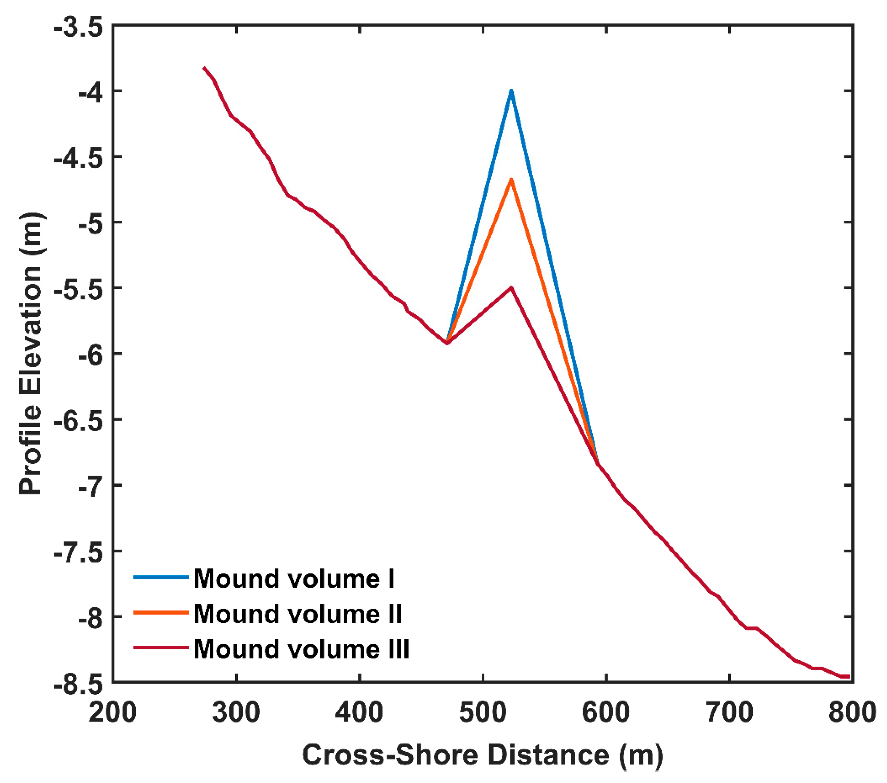
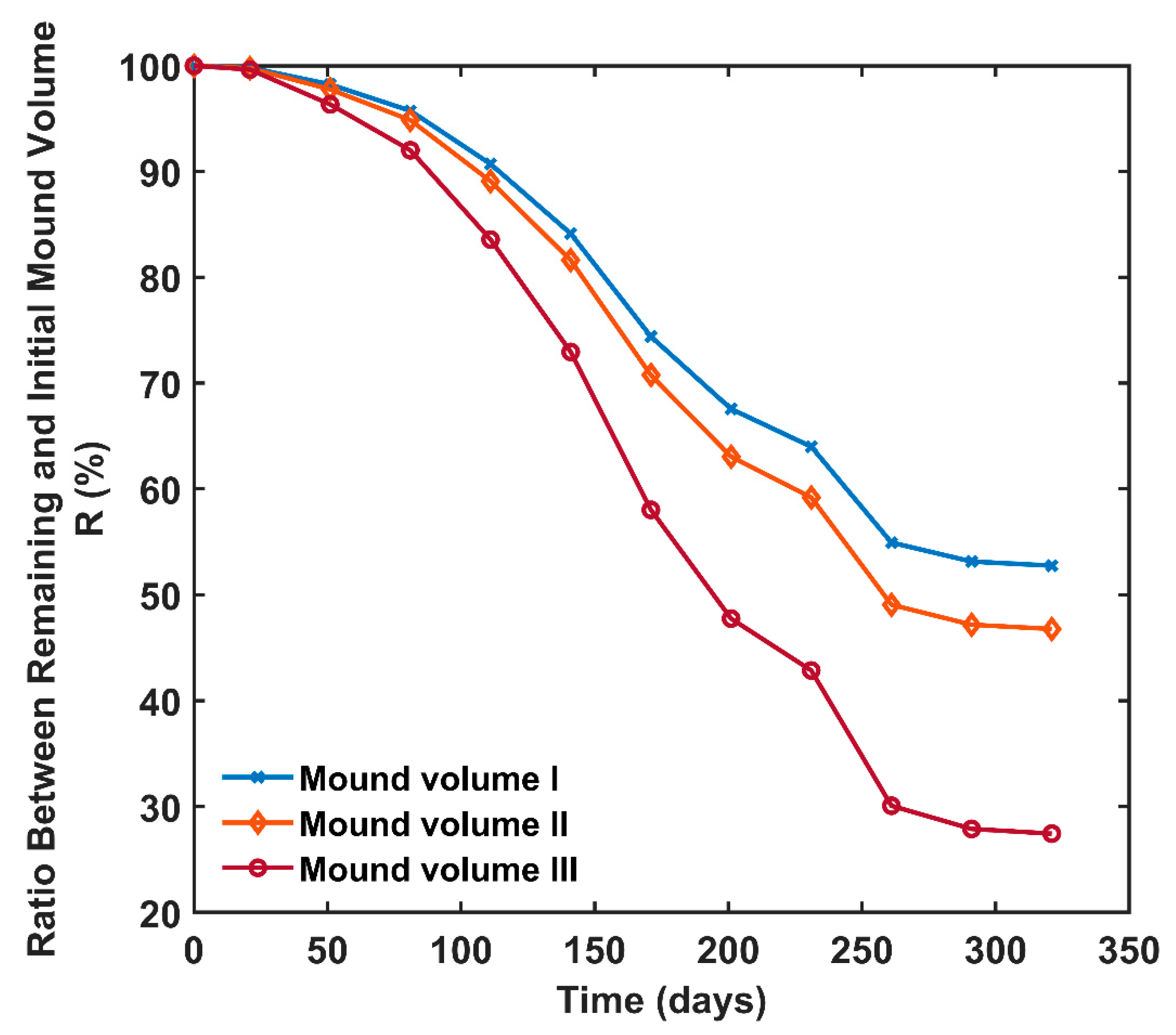
3.3.1. Effect of Mound Volume

Figure 9 illustrates the initial mound shapes employed and how they differed in volume, whereas Figure 10 shows the decrease in time of R as a result of mound diffusion. Viewing Figure 9 and Figure 10 together, it can be seen that the diffusion rate for all mounds with different initial volume are increasing with time in the beginning and then decreasing to a small value, approaching a zero rate, indicating that the mound spreads out fast at first and then slowly until equilibrium is reached. In addition, the ratio R changes the fastest for the smallest mound and the slowest for the largest mound, which implies that the smaller the mound, the higher the relative diffusion rate.

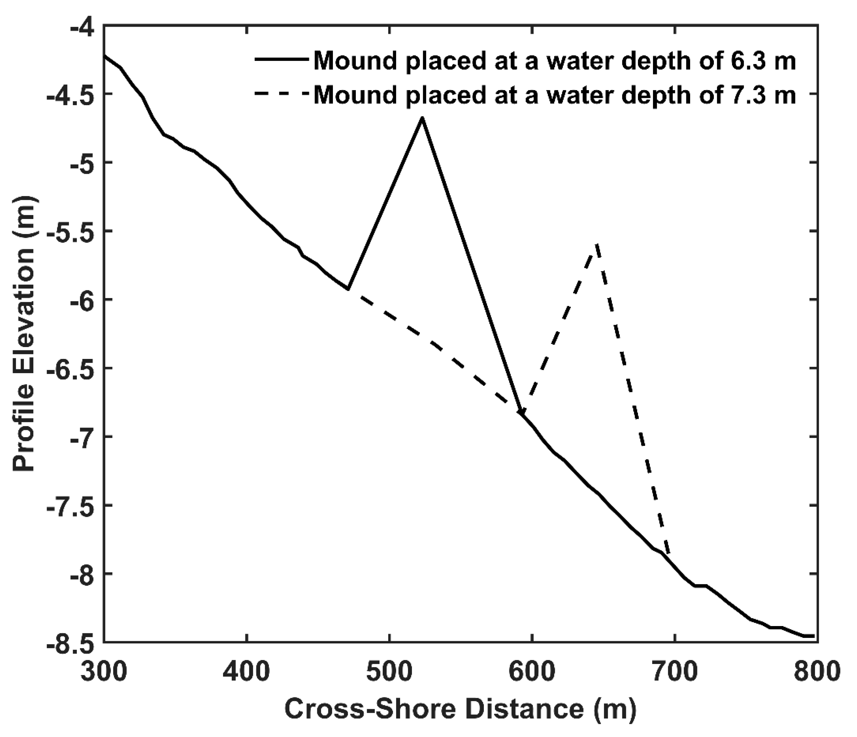
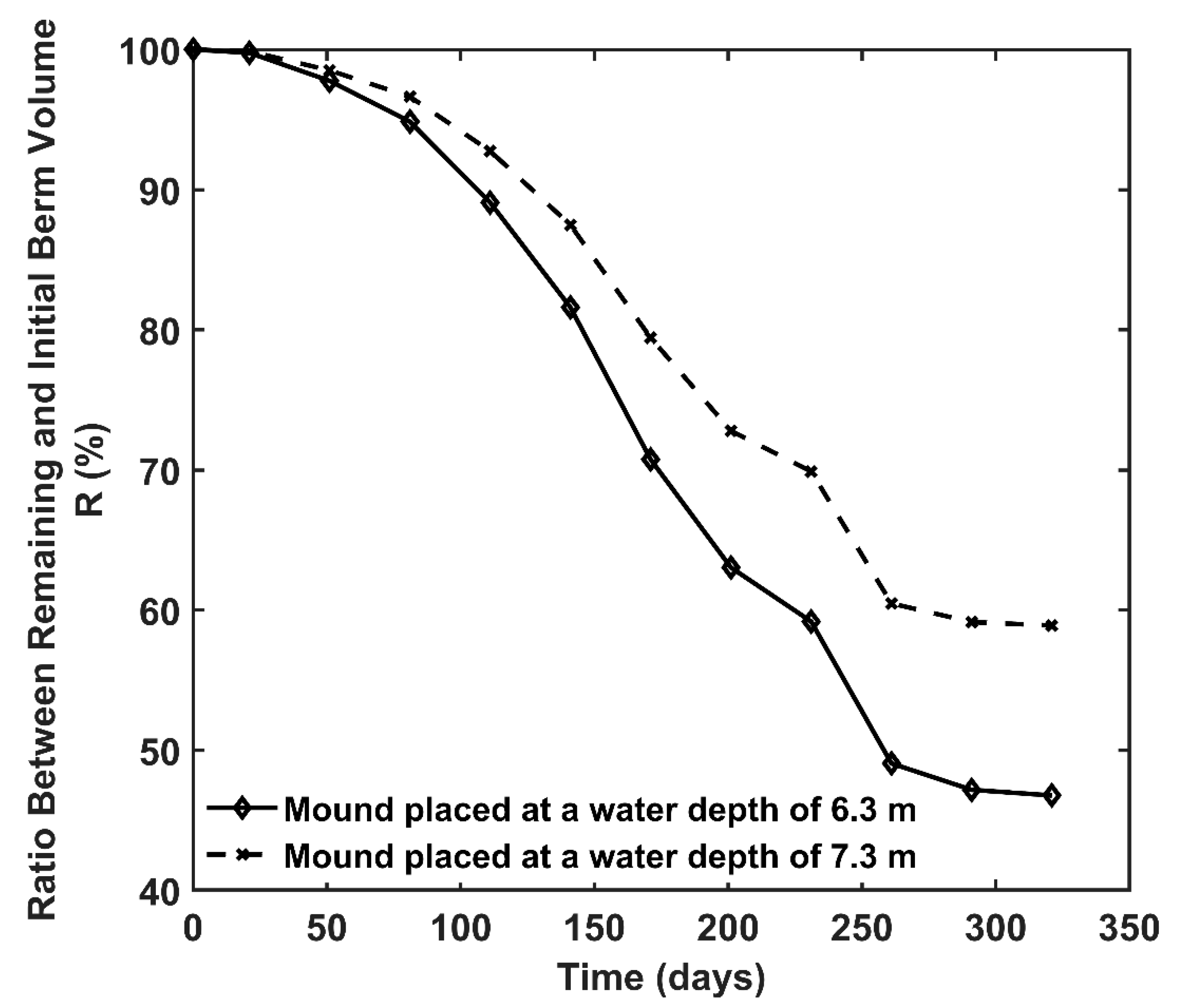
3.3.2. Effect of Mound Placement

Figure 11 displays two different mound placements, having the same initial volume but located at different depths, and Figure 12 shows the variation in R with time. By considering Figure 11 and Figure 12 simultaneously, it may be seen that the rates of mound diffusion firstly increase and then decline for both mounds, independently of the water depth. However, the rate for the mound at a water depth of 7.3 m is slower than the mound at a water depth of 6.3 m (depths a center of mound, prefill conditions), illustrating the mound in deeper water is not as active from a transport point of view, which is consistent with previous studies by other researchers. This type of simulation results can assist coastal engineers and managers to design stable or active mounds according to their requirements.

4. Discussion

In this section, the novelty of the model for simulating the evolution of offshore mounds is first discussed, then some further model improvements for applications in the future are proposed.

4.1. The Novelty of the Model

Beach nourishment has become the preferred remedy against coastal erosion in recent years. However, to select the optimal design and placement of mounds, as well as to predict the evolution of the placed material, are challenges to coastal engineers and managers but of great significance.

In this study, a new numerical model was developed to simulate the response of a placed mound in the offshore to varying waves and water levels. The model was based on the work by Zhang, Larson, and Ge [28], where an enhanced formula for calculating the transport in the offshore was developed and included in the model. The transport in the offshore was assumed to be primarily bed load and the effects of wave asymmetry were included employing first-order cnoidal theory. In addition, the previous model did not explicitly include the equilibrium properties of the beach profile, which is typically needed when simulating over long time periods. Thus, the equilibrium bed slope was considered in the new transport equation, which makes the model suitable for long-term simulations of mound evolution in the offshore, yielding reliable and robust results.

The model was applied to two field sites with detailed measurements on the evolution of offshore mounds. The simulation results showed good agreement with the measurements without any calibration, employing standard values on the parameters in the derived transport equation. This provided additional credibility to the model and indicates the possibility to apply it at other sites with a minimum of calibration. Other models have previously predicted the behavior of morphological features in the offshore, including both advanced numerical models [45] and simpler empirical predictive equations [46], but these models have emphasized natural features such as longshore bars. Thus, the new model constitutes a useful tool to study offshore mounds that represent a feature not naturally occurring at a site.

4.2. Futher Improvements of the Model

As previously pointed out, the model simulates the sediment transport by non-breaking waves, implying that the transport induced by undertow is not considered. This restricts the model to simulate mound evolution outside the surf zone, where wave breaking is negligible. In addition, although breaking waves may be limited, a return flow along the bottom may occur due to the Stokes drift; this possible mechanism for transport is also ignored at present as well as any contribution from boundary layer streaming. In addition, phase-lag effects are not described since they tend to be most pronounced at sheet-flow conditions, which typically did not prevail in the present cases. The latter was checked by comparing the condition at the mound with a criterion for sheet flow [47]; only for a few events were this criterion exceeded and the mound evolution was dominated by non-sheet flow conditions. Phase-lag effects may be introduced using the method proposed by Camenen and Larson [47].

Furthermore, the effects of longshore sediment transport are not included in the model, which means that possible longshore gradients that can cause changes in the profile shape are ignored, especially at the ends of the fill. In the comparison with measured profile evolution, surveyed profiles in the center of the fills were employed to avoid these effects. Thus, the present model is most applicable to the central part of a mound that are placed in the offshore, parallel to the shore, and with a certain alongshore extent. In the next step of the modeling, sediment transport induced by undertow should be included and the longshore sediment transport should be taken into account, in order to allow for simulation of mound evolution under more general condition, particularly in the nearshore.

In the design section studying schematized mounds, only the evolution of triangular-shaped mounds was investigated and for a limited set of parameters. Additionally, the mounds were given the same width implying larger mound volumes as the height was increased. According to analytical solutions presented in the study by Larson and Hanson [15], a mound with twice the width will require four times as long period of the wave action to experience the same relative spread; thus, the effect of mound width to the mound evolution should be simulated as well in a more comprehensive study.

Thus, some other mound shapes and their geometrical design, such as rectangular shapes, should be investigated with the model in the next step, since Dean [11] established that the mound evolution is dependent on the relative mound width for a rectangular beach fill.

Therefore, in the future, some other simulations should be carried out for other mound designs in a more systematic way to establish guidelines for determining the most suitable design for preliminary assessments in the initial phase of nourishment projects involving offshore mounds.

In addition, other sediment transport formula suitable to describe offshore mound evolution should be tested and compared with predictions by the present model.

5. Conclusions

A numerical model for simulating the evolution of offshore mounds due to varying waves and water levels, where non-breaking waves prevail concerning the transport and wave asymmetry is important, was developed. The equilibrium profile was integrated into transport equation for the net sediment transport rate, which is based on bed load being predominant. In order to test the model, data from two field sites involving mound placement, Cocoa Beach and Perdido Key Beach in Florida, were employed for model comparison. The simulation results were in good agreement with the measured data without any particular calibration using standard values, indicating that the model is sufficiently reliable and robust to simulate the evolution of mounds placed in the offshore. In addition, for the purpose of exploring the influence of mound design, such as volume and location (i.e., placement depth), on mound evolution, different scenarios based on the data set from Cocoa Beach were simulated. The results showed behavior consistent with previously conducted studies, which further supports the usefulness of the model in simulating offshore mound evolution.

References

1. Bruun, P. Design and Construction of Mounds for Breakwaters and Coastal Protection; Elsevier: Amsterdam, The Netherlands, 2013; Volume 37. [Google Scholar]
2. Thomas, R.; Hall, B. Seawall Design; Butterworth-Heinemann: Oxford, UK, 2015. [Google Scholar]
3. Pilarczyk, K. Dikes and Revetments: Design, Maintenance and Safety Assessment; Routledge: Abingdon-on-Thames, UK, 2017. [Google Scholar]
4. Airoldi, L.; Abbiati, M.; Beck, M.W.; Hawkins, S.J.; Jonsson, P.R.; Martin, D.; Moschella, P.S.; Sundelöf, A.; Thompson, R.C.; Åberg, P. An ecological perspective on the deployment and design of low-crested and other hard coastal defence structures. Coast. Eng. 2005, 52, 1073–1087. [Google Scholar] [CrossRef] [Green Version]
5. Simberloff, D. How common are invasion-induced ecosystem impacts? Biol. Invasions 2011, 13, 1255–1268. [Google Scholar] [CrossRef]
6. Firth, L.; Thompson, R.; Bohn, K.; Abbiati, M.; Airoldi, L.; Bouma, T.; Bozzeda, F.; Ceccherelli, V.; Colangelo, M.; Evans, A. Between a rock and a hard place: Environmental and engineering considerations when designing coastal defence structures. Coast. Eng. 2014, 87, 122–135. [Google Scholar] [CrossRef] [Green Version]
7. Charlier, R.H.; De Meyer, C.P. Beach nourishment as efficient coastal protection. Environ. Manag. Health 1995, 6, 26–34. [Google Scholar] [CrossRef]
8. Hamm, L.; Capobianco, M.; Dette, H.; Lechuga, A.; Spanhoff, R.; Stive, M. A summary of European experience with shore nourishment. Coast. Eng. 2002, 47, 237–264. [Google Scholar] [CrossRef]
9. Hanson, H.; Brampton, A.; Capobianco, M.; Dette, H.; Hamm, L.; Laustrup, C.; Lechuga, A.; Spanhoff, R. Beach nourishment projects, practices, and objectives—A European overview. Coast. Eng. 2002, 47, 81–111. [Google Scholar] [CrossRef]
10. Dean, R.G. Beach Nourishment: Theory and Practice; World Scientific Publishing Company: Singapore, 2003; Volume 18. [Google Scholar]
11. Dean, R.G. Principles of beach nourishment. In Handbook of Coastal Processes and Erosion; CRC Press: Boca Raton, FL, USA, 2018; pp. 217–232. [Google Scholar]
12. Barnard, P.L.; Hanes, D.M.; Lescinski, J.; Elias, E. Monitoring and modeling nearshore dredge disposal for indirect beach nourishment, Ocean Beach, San Francisco. In Coastal Engineering 2006; World Scientific: Singapore, 2007; Volume 5, pp. 4192–4204. [Google Scholar]
13. Foster, G.; Healy, T.; de Lange, W. Presaging beach renourishment from a nearshore dredge dump mound, Mt. Maunganui Beach New Zealand J. Coast. Res. 1996, 12, 395–405. [Google Scholar]
14. Larson, M.; Ebersole, B.A. An Analytical Model to Predict the Response of Mounds Placed in the Offshore; Engineer Research and Development Center Vicksburg Ms Coastal and Hydraulics Lab: Vicksburg, MS, USA, 1999. [Google Scholar]
15. Larson, M.; Hanson, H. Model of the evolution of mounds placed in the nearshore. Rev. Gestão Costeira Integr. J. Integr. Coast. Zone Manag. 2015, 15, 21–33. [Google Scholar] [CrossRef]
16. McLellan, T.N. Nearshore mound construction using dredged material. J. Coast. Res. 1990, SI:7, 99–107. [Google Scholar]
17. Smith, E.R.; D’Alessandro, F.; Tomasicchio, G.R.; Gailani, J.Z. Nearshore placement of a sand dredged mound. Coast. Eng. 2017, 126, 1–10. [Google Scholar] [CrossRef]
18. Smith, E.R.; Mohr, M.C.; Chader, S.A. Laboratory experiments on beach change due to nearshore mound placement. Coast. Eng. 2017, 121, 119–128. [Google Scholar] [CrossRef]
19. Smith, E.R.; Permenter, R.; Mohr, M.C.; Chader, S.A. Modeling of Nearshore-Placed Dredged Material; Engineer Research and Development Center Vicksburg Ms Coastal and Hydraulics Lab: Vicksburg, MS, USA, 2015. [Google Scholar]
20. Hall, J.; Herron, W. Test of Nourishment of the Shore by Offshore Deposition of Sand, Long Branch, New Jersey; Corps of Engineers Washington DC Beach Erosion Board: Washington, DC, USA, 1950. [Google Scholar]
21. Otay, E. Long Term Evolution of Disposal Berms; University of Florida: Gainesville, FL, USA, 1994. [Google Scholar]
22. Van Rijn, L.; Walstra, D. Analysis and Modelling of Shoreface Nourishments; Deltares (WL): Delft, The Netherlands, 2004. [Google Scholar]
23. Browder, A.E.; Dean, R.G. Monitoring and comparison to predictive models of the Perdido Key beach nourishment project, Florida, USA. Coast. Eng. 2000, 39, 173–191. [Google Scholar] [CrossRef]
24. McLellan, T.N.; Kraus, N.C. Design guidance for nearshore berm construction. In Coastal Sediments; ASCE: Reston, VA, USA, 1991; pp. 2000–2011. [Google Scholar]
25. Douglass, S.L. Estimating landward migration of nearshore constructed sand mounds. J. Waterw. Port Coast. Ocean. Eng. 1995, 121, 247–250. [Google Scholar] [CrossRef]
26. Van Duin, M.; Wiersma, N.; Walstra, D.; Van Rijn, L.; Stive, M. Nourishing the shoreface: Observations and hindcasting of the Egmond case, The Netherlands. Coast. Eng. 2004, 51, 813–837. [Google Scholar] [CrossRef]
27. McFall, B.C.; Smith, S.J.; Pollock, C.E.; Rosati, J., III; Brutsche, K.E. Evaluating Sediment Mobility for Siting Nearshore Berms; US Army Engineer Research and Development Center Vicksburg United States: Vicksburg, MS, USA, 2016. [Google Scholar]
28. Zhang, J.; Larson, M.; Ge, Z.P. Numerical model of beach profile evolution in the nearshore. J. Coast. Res. 2020. [Google Scholar] [CrossRef]
29. Larson, M. Model for decay of random waves in surf zone. J. Waterw. Port Coast. Ocean. Eng. 1995, 121, 1–12. [Google Scholar] [CrossRef]
30. Rattanapitikon, W.; Shibayama, T. Simple model for undertow profile. Coast. Eng. J. 2000, 42, 1–30. [Google Scholar] [CrossRef]
31. Kraus, N.C.; Smith, J.M. SUPERTANK Laboratory Data Collection Project; TR-CERC-94-3; USACE-WES: Vicksburg, MS, USA, 1994. [Google Scholar]
32. Isobe, M. Calculation and application of first-order cnoidal wave theory. Coast. Eng. 1985, 9, 309–325. [Google Scholar] [CrossRef]
33. Camenen, B.; Larson, M. A bedload sediment transport formula for the nearshore. Estuar. Coast. Shelf Sci. 2005, 63, 249–260. [Google Scholar] [CrossRef]
34. Grasmeijer, B.; Ruessink, B. Modeling of waves and currents in the nearshore parametric vs. probabilistic approach. Coast. Eng. 2003, 49, 185–207. [Google Scholar] [CrossRef]
35. Isobe, M.; Horikawa, K. Study on water particle velocities of shoaling and breaking waves. Coast. Eng. Jpn. 1982, 25, 109–123. [Google Scholar] [CrossRef]
36. Madsen, O.S. Mechanics of cohesionless sediment transport in coastal waters. In Coastal Sediments; ASCE: Reston, VA, USA, 1991; pp. 15–27. [Google Scholar]
37. Madsen, O. Sediment transport on the shelf. In Sediment Transport Workshop DRP TA1; Coastal Engineering Research Center: Vicksburg, MS, USA, 1993. [Google Scholar]
38. Hearin, J. Historical analysis of beach nourishment and its impact on the morphological modal beach state in the North Reach of Brevard County, Florida. J. Coast. Mar. Res. 2014, 2, 37–53. [Google Scholar] [CrossRef]
39. Hearin, J.M. A Detailed Analysis of Beach Nourishment and Its Impact on the Surfing Wave Environment of Brevard County, Florida; Florida Institute of Technology: Melbourne, FL, USA, 2012. [Google Scholar]
40. The Wave Information Study (WIS). Available online: http://wis.usace.army.mil/ (accessed on 17 January 2020).
41. Work, P. Perdido Key Beach Nourishment Project: Gulf Islands National Seashore (Pre-Nourishment Survey-Conducted 28 October–3 November 1989); Coastal and Oceanographic Engineering Department, University of Florida: Gainesville, FL, USA, 1990. [Google Scholar]
42. Dean, R.G. Recommendations for Placement of Dredged Sand on Perdido Key Gulf Islands National Seashore; University of Florida Coastal and Oceanographic Engineering Department: Gainesville, FL, USA, 1988. [Google Scholar]
43. Work, P.A.; Otay, E.N. Influence of nearshore berm on beach nourishment. In Coastal Engineering 1996; ASCE: Reston, VA, USA, 1997; pp. 3722–3735. [Google Scholar]
44. WXTide32. Available online: https://wxtide32.informer.com/4.6/ (accessed on 17 February 2020).
45. Roelvink, J.; Stive, M. Bar-generating cross-shore flow mechanisms on a beach. J. Geophys. Res. Ocean. 1989, 94, 4785–4800. [Google Scholar] [CrossRef]
46. Larson, M.; Kraus, N.C. Analysis of Cross-Shore Movement of Natural Longshore Bars and Material Placed to Create Longshore Bars; Technical Report DRP92-5; Coastal Engineering Research Center, U.S. Army Engineer Waterways Experiment Station: Vicksburg, MS, USA, 1992. [Google Scholar]
47. Camenen, B.; Larson, M. Phase-lag effects in sheet flow transport. Coast. Eng. 2006, 53, 531–542. [Google Scholar] [CrossRef]
Figure 1. Non-dimensional transport coefficient (Kn) as a function of the Ursell number (Ur) and two polynomial least-square fits to different parts of the theoretical curve.
Jmse 08 00160 g001
Figure 2. Comparisons between measured and calculated profiles 136 days after the mound placement, Cocoa Beach.
Jmse 08 00160 g002
Figure 3. Comparisons between measured and calculated profiles 291 days after the mound placement, Cocoa Beach.
Jmse 08 00160 g003
Figure 4. The evolution of the mound with time.
Jmse 08 00160 g004
Figure 5. The distribution of the total sediment transport rate across the profile at different times.
Jmse 08 00160 g005
Figure 6. (a) The evolution of the mound after 136 days in response to changes in the values of the parameter CTAS used as a multiplier for the bed load sediment transport rate. (b) The evolution of the mound after 291 days in response to changes in the values of the parameter CTAS used as a multiplier for the bed load sediment transport rate.
Jmse 08 00160 g006aJmse 08 00160 g006b
Figure 7. Calculated and measured profiles one year after mound disposal at the midpoint of mound.
Jmse 08 00160 g007
Figure 8. Calculated and measured profiles one year after mound disposal for Range 58.
Jmse 08 00160 g008
Figure 9. Studied schematized triangular mounds having different initial volumes.
Jmse 08 00160 g009
Figure 10. The ratio change between remaining and initial mound volume with time.
Jmse 08 00160 g010
Figure 11. Studied schematized triangular mounds placed at different water depths, but having the same initial volume.
Jmse 08 00160 g011
Figure 12. The ratio change between remaining and initial mound volume over time.
Jmse 08 00160 g012