Robust Capon Beamforming against Steering Vector Error Dominated by Large Direction-of-Arrival Mismatch for Passive Sonar

Abstract

Capon beamforming is often applied in passive sonar to improve the detectability of weak underwater targets. However, we often have no accurate prior information of the direction-of-arrival (DOA) of the target in the practical applications of passive sonar. In this case, Capon beamformer will suffer from performance degradation due to the steering vector error dominated by large DOA mismatch. To solve this, a new robust Capon beamforming approach is proposed. The essence of the proposed method is to decompose the actual steering vector into two components by oblique projection onto a subspace and then estimate the actual steering vector in two steps. First, we estimate the oblique projection steering vector within the subspace by maximizing the output power while controlling the power from the sidelobe region. Subsequently, we search for the actual steering vector within the neighborhood of the estimated oblique projection steering vector by maximizing the output signal-to-interference-plus-noise ratio (SINR). Semidefinite relaxation and Charnes-Cooper transformation are utilized to derive convex formulations of the estimation problems, and the optimal solutions are obtained by the rank-one decomposition theorem. Numerical simulations demonstrate that the proposed method can provide superior performance, as compared with several previously proposed robust Capon beamformers in the presence of large DOA mismatch and other array imperfections.

1. Introduction

Underwater target detection is a primordial task for passive sonar systems. In practical underwater environments, the presence of the strong underwater targets will severely affect the detection performance of the weak targets. Therefore, the strong targets are considered as interferences for the weak targets. Capon beamforming [1,2], as an important pre-processing technique in array signal processing, is often applied in passive sonar arrays for improving the detectability of weak underwater targets [3,4,5]. By extracting the signal of weak targets and suppressing the strong interferences and noise at the beamformer output simultaneously, Capon beamformer can obtain the optimal output signal-to-interference-plus-noise ratio (SINR) and prevent the weak sources from submerging in strong interferences. However, due to some imperfections in practice, such as direction-of-arrival (DOA) mismatch, imperfect array element calibration, and distorted array shape [6,7,8], the knowledge of the actual steering vector can be inaccurate, which will cause a substantial degradation in the performance of Capon beamforming.

In recent years, various approaches have been developed to improve the robustness of Capon beamformer against the steering vector error. Generally, these approaches can be classified into two categories: The robust constrained approach and the steering vector estimation approach. In the robust constrained approach, such as the worst-case performance optimization-based approach [9] and the doubly constrained approach [10,11], the uncertainty constraints on the array magnitude response or the steering vector error are usually imposed without estimating the actual steering vector. However, in the case of large steering vector error, a large size of uncertainty set is required in the robust constrained approach which will weaken the abilities of interference-plus-noise suppression. On the other hand, the main-lobe of robust constrained beamformer usually points to the presumed DOA of the signal rather than the actual DOA. Unlike the robust constrained approach, the steering vector estimation approach searches for the actual steering vector directly based on some prior information. The most typical beamformer based on steering vector estimation is the so-called eigenspace-based beamformer (ESB) [12], where the actual steering vector can be well estimated by utilizing the signal-plus-interference subspace. The ESB is considered to be one of the most powerful techniques robust to arbitrary steering vector mismatch case [9]. Nevertheless, it will suffer from severe performance degradation if the dimension of the signal-plus-interference subspace is misestimated. To solve this problem, some improved steering vector estimation approaches were proposed. In Reference [13], the actual steering vector is estimated iteratively where a quadratic convex optimization problem is solved at each iteration. The main drawback of this method is the high computational complexity due to the iterations. In Reference [14], a nonconvex quadratically constrained quadratic programming (QCQP) problem and the corresponding relaxation procedure were developed to estimate the actual steering vector. As compared with the beamformer in Reference [13], this method has more degrees of freedom and achieves superior performance.

This paper mainly focuses on improving the robustness of Capon beamformer against the steering vector error dominated by large DOA mismatch. This type of steering vector error is very common in the practical applications of passive sonar, where the accurate prior information of the DOA of the signal is usually unavailable [15]. In this case, large DOA mismatch is naturally dominant in the steering vector error, but other array imperfections can also occur. Besides the beamformers discussed above, some robust Capon beamformers specially developed to improve the robustness against the steering vector error dominated by large DOA mismatch have been proposed. Generally, these beamformers belong to the steering vector estimation approach. In Reference [16], the actual steering vector is considered to lie in the intersection of two constructed subspaces and can be estimated by the alternating projection algorithm. However, similar to the ESB, an incorrect estimation of the dimension of signal-plus-interference subspace will cause performance degradation. In Reference [17], a robust Capon beamforming method against large DOA mismatch was proposed. This method expresses the actual steering vector as a linear combination of the columns of a subspace and estimate the coefficients by maximizing the output power. However, this beamformer lacks robustness against other array imperfections. To solve this, an improved beamformer was proposed in Reference [18]. By employing the general-rank signal model-based robust beamforming technique [19], this beamformer provides further robustness against other array imperfections.

In this paper, we develop a new approach to robust Capon beamforming in the presence of large DOA mismatch and other array imperfections. Our approach is based on the two-step estimation of the actual steering vector. By projecting the actual steering vector obliquely onto a subspace, we can decompose the actual steering vector into two components and then search for them within the subspace and the neighborhood of the oblique projection steering vector, respectively. It turns out the natural formulations of the two estimation problems all involve nonconvex objective function or nonconvex constraint, and therefore are NP-hard to solve. To mitigate this problem, we utilize the semidefinite relaxation technique [20] and Charnes-Cooper transformation technique [21] to derive convex formulations of two estimation problems, and obtain the optimal solutions by applying the rank-one decomposition theorem [22]. Numerical simulations show that the performance of the proposed beamformer is always close to the optimal value in the presence of large DOA mismatch and other array imperfections.

This paper is organized as follows. In Section 2, the array signal model and some backgrounds on Capon beamforming are introduced. In Section 3, the new robust Capon beamforming method is proposed. In Section 4, simulation results are presented to demonstrate the effectiveness of the proposed method. Finally, the paper is concluded in Section 5.

2. Backgrounds

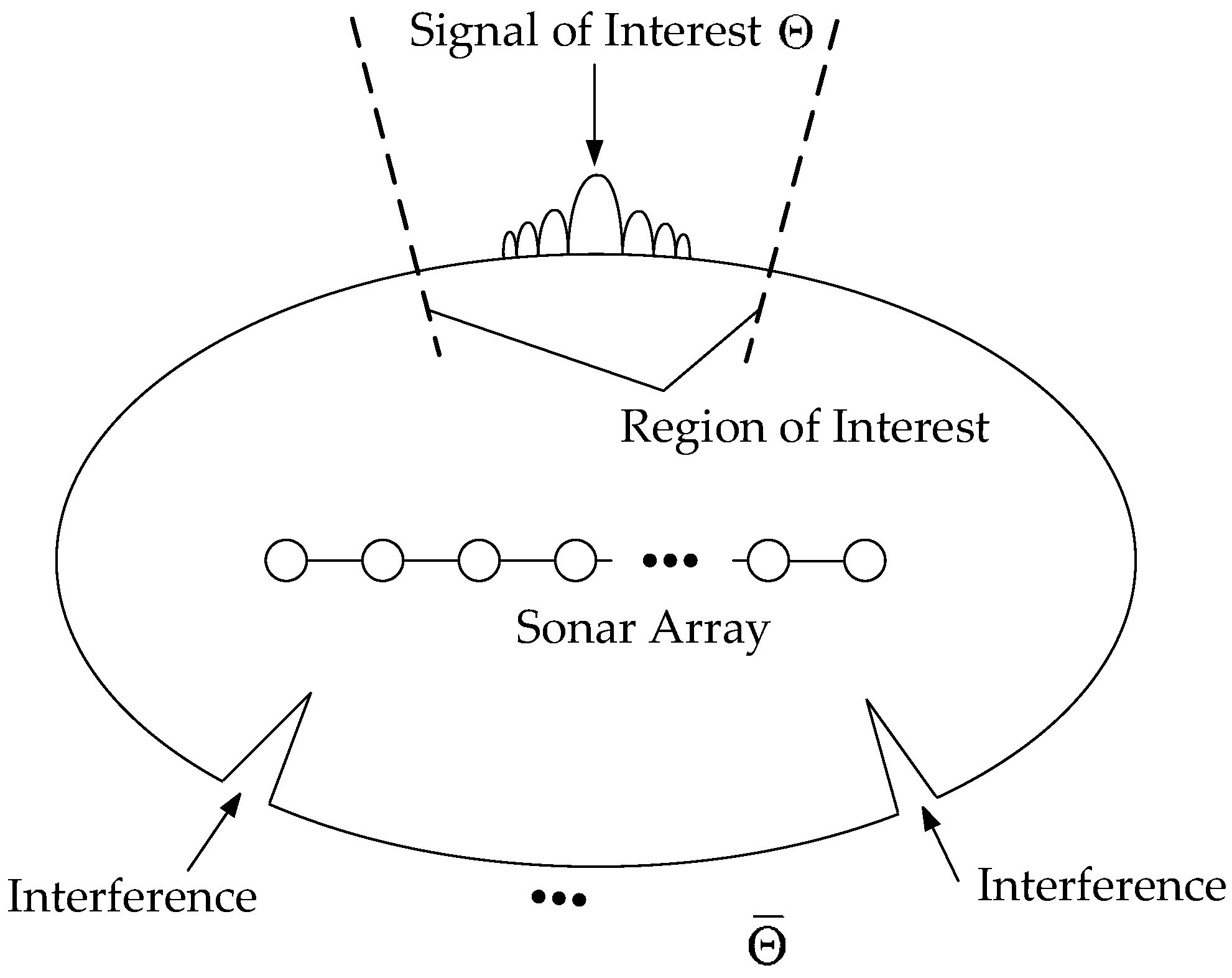
2.1. Array Signal Model

Consider a linear sonar array with $M$ omnidirectional elements receiving narrowband signals from $D(D<M)$ far-field underwater targets (one desired signal and $D-1$ interferences). The depiction on the array signal model is shown in Figure 1. The $k$th array snapshot vector $x(k)\in {ℂ}^M$ can be modeled as:

$$x(k)=x_s(k)+x_{\mathrm{int}}(k)+n(k)$$

(1)

where $x_s(k)$, $x_{\mathrm{int}}(k)$, and $n(k)$ denote the signal of interest (SOI), interference and noise components, respectively. The SOI can be written as $x_s(k)=a{s}_0(k)$, where $a$ is the steering vector associated with the SOI and $s_0(k)$ is the waveform of the SOI. The interferences can be written as $x_{\mathrm{int}}(k)={\displaystyle \sum _{i=1}^{D-1}{a}_i{s}_i(k)}$, where $a_i$ and $s_i(k)$ denote the steering vector and the waveform of the $i$th interference, respectively. The additive noise $n(k)$ is modeled as a zero-mean spatially and temporally white Gaussian process with the power ${\sigma }_n^2$. Here, the SOI, interferences, and noise are statistically independent with each other. As shown in Figure 1, we define an angular region of interest (ROI) $\mathrm{\Theta }$ and its complementary region $\overline{\mathrm{\Theta }}$, that is, $\mathrm{\Theta }\cup \overline{\mathrm{\Theta }}$ covers the whole spatial domain and $\mathrm{\Theta }\cap \overline{\mathrm{\Theta }}$ is empty. The main required prior information is that the SOI is located in $\mathrm{\Theta }$ while the interferences are not, which implies that the accurate DOA of the SOI is not required. Consequently, the DOA uncertainty set is $\mathrm{\Theta }$ which leads to a large DOA mismatch scenario.

2.2. Capon Beamforming

The output of a beamformer is given by:

$$y(k)=w^{H}x(k)$$

(2)

where $w={\left[w_1,w_2,\cdots ,w_M\right]}^T\in {ℂ}^M$ is the complex weight vector, ${(·)}^T$ and ${(·)}^H$ denote the transpose and Hermitian transpose, respectively. The output SINR of a beamformer is defined as:

$${\mathrm{SINR}}_{\mathrm{out}}=\frac{E\left\{{\left|w^H{x}_s(k)\right|}^2\right\}}{E\left\{{\left|w^H(x_{\mathrm{int}}(k)+n(k))\right|}^2\right\}}=\frac{{\sigma }_0^2{\left|w^{H}a\right|}^2}{w^H{R}_{i+n}w}$$

(3)

where ${\sigma }_0^2=E\left\{{\left|s_0(k)\right|}^2\right\}$ is the power of the SOI, $R_{i+n}=E\{(x_{\mathrm{int}}(k)+n(k)){(x_{\mathrm{int}}(k)+n(k))}^H\}$ is the interference-plus-noise covariance matrix and $E\{·\}$ denotes the statistical expectation. The Capon beamformer aims at maximizing the output SINR by maintaining a distortionless response towards the SOI and minimizing the output power of interference-plus-noise. Therefore, the Capon beamformer is equivalent to:

$$\underset{w}{\min }{w}^H{R}_{i+n}w\mathrm{subject}\mathrm{to}{w}^{H}a=1$$

(4)

Based on the statistical independence among the SOI, interferences, and noise, we can easily obtain that:

$$R_x=E\left\{x(k)x^H(k)\right\}={\sigma }_0^{2}a{a}^H+R_{i+n}$$

(5)

$$w^H{R}_{x}w=w^H{R}_{i+n}w+{\sigma }_0^2{\left|w^{H}a\right|}^2$$

(6)

Hence, Problem (4) is equivalent to:

$$\underset{w}{\min }{w}^H{R}_{x}w\mathrm{subject}\mathrm{to}{w}^{H}a=1$$

(7)

The optimal solution to Problem (7) yields to the weight of standard Capon beamformer (SCB) [2]:

$$w=\frac{R_x^{-1}a}{a^H{R}_x^{-1}a}$$

(8)

In practical applications, $R_x$ is usually unavailable and replaced by the sample covariance matrix:

$${\widehat{R}}_x=\frac{1}{N}{\displaystyle \sum _{k=1}^{N}x(k)x^H(k)}$$

(9)

where $N$ is the number of snapshots.

2.3. Effects of Steering Vector Error

It is worth noting that the weight of SCB is based on the assumption that the steering vector of the SOI is accurately known. In practice, factors such as DOA mismatch and array imperfections (including array element calibration errors and position errors) can lead to an error between the presumed steering vector and the actual steering vector, i.e.:

$$a=\overline{a}+e$$

(10)

where $\overline{a}$ is the presumed steering vector and $e$ is an unknown error vector. The weight vector of SCB, when using the sample covariance matrix ${\widehat{R}}_x$ and the presumed steering vector $\overline{a}$, is then given by:

$$w=\frac{{\widehat{R}}_x^{-1}\overline{a}}{{\overline{a}}^H{\widehat{R}}_x^{-1}\overline{a}}$$

(11)

With Problem (11), the array response at the direction of the SOI can be expressed as follows:

$$H\left(a\right)=\left|w^{H}a\right|=\frac{\left|{\overline{a}}^H{\widehat{R}}_x^{-1}a\right|}{\left|{\overline{a}}^H{\widehat{R}}_x^{-1}\overline{a}\right|}=\frac{\left|{\overline{a}}^{H}V{V}^{H}a\right|}{\left|{\overline{a}}^{H}V{V}^H\overline{a}\right|}$$

(12)

where $V\triangleq {\widehat{R}}_x^{-1/2}$. Applying the Cauchy-Schwarz inequality, we have that:

$$\left|{\overline{a}}^{H}V{V}^{H}a\right|\le \Vert a^{H}V\Vert \Vert {\overline{a}}^{H}V\Vert$$

(13)

where $\Vert ·\Vert$ denotes the 2-norm operation. By substituting Problem (13) into Problem (12), we can write that:

$$H\left(a\right)\le \frac{\Vert a^{H}V\Vert \Vert {\overline{a}}^{H}V\Vert }{{\Vert {\overline{a}}^{H}V\Vert }^2}=\frac{\Vert a^{H}V\Vert }{\Vert {\overline{a}}^{H}V\Vert }=\frac{\sqrt{1/{\overline{a}}^H{\widehat{R}}_x^{-1}\overline{a}}}{\sqrt{1/a^H{\widehat{R}}_x^{-1}a}}$$

(14)

Based on the Capon spatial spectrum estimator [1], $1/a^H{\widehat{R}}_x^{-1}a$ and $1/{\overline{a}}^H{\widehat{R}}_x^{-1}\overline{a}$ can be considered as the power collected from the directions of the SOI and the presumed steering vector, respectively. Also, it is easy to know that $1/a^H{\widehat{R}}_x^{-1}a$ can be approximated as the power of SOI-plus-noise. Since the Capon estimator has high resolution in spectrum estimation, $1/a^H{\widehat{R}}_x^{-1}a$ will deviate from $1/{\overline{a}}^H{\widehat{R}}_x^{-1}\overline{a}$ as long as the steering vector error occurs between $a$ and $\overline{a}$, resulting in the distortion of the array response. Particularly when large steering vector error occurs, $1/{\overline{a}}^H{\widehat{R}}_x^{-1}\overline{a}$ can be approximated as the power of noise only. In this case, the value of $H\left(a\right)$ will decrease as the signal-to-noise ratio (SNR) increases, which means the enhancement of the distortion at the direction of the SOI. The enhanced distortion can cause the signal self-nulling phenomenon [13].

As we discussed in Section 1, the steering vector error caused by large DOA mismatch is dominant in the applications of passive sonar systems. Motivated by this fact, this paper mainly focuses on estimating the actual steering vector to improve the robustness of Capon beamformer in the case of large DOA mismatch, but unlike the beamformer in Reference [17], other array imperfections are also taken into consideration.

3. Proposed Method

Our approach is based on the two-step steering vector estimation. We begin with the decomposition of the actual steering vector and then formulate two optimization problems to estimate the actual steering vector in two steps. The corrected beam can be formed by using the estimated actual steering vector.

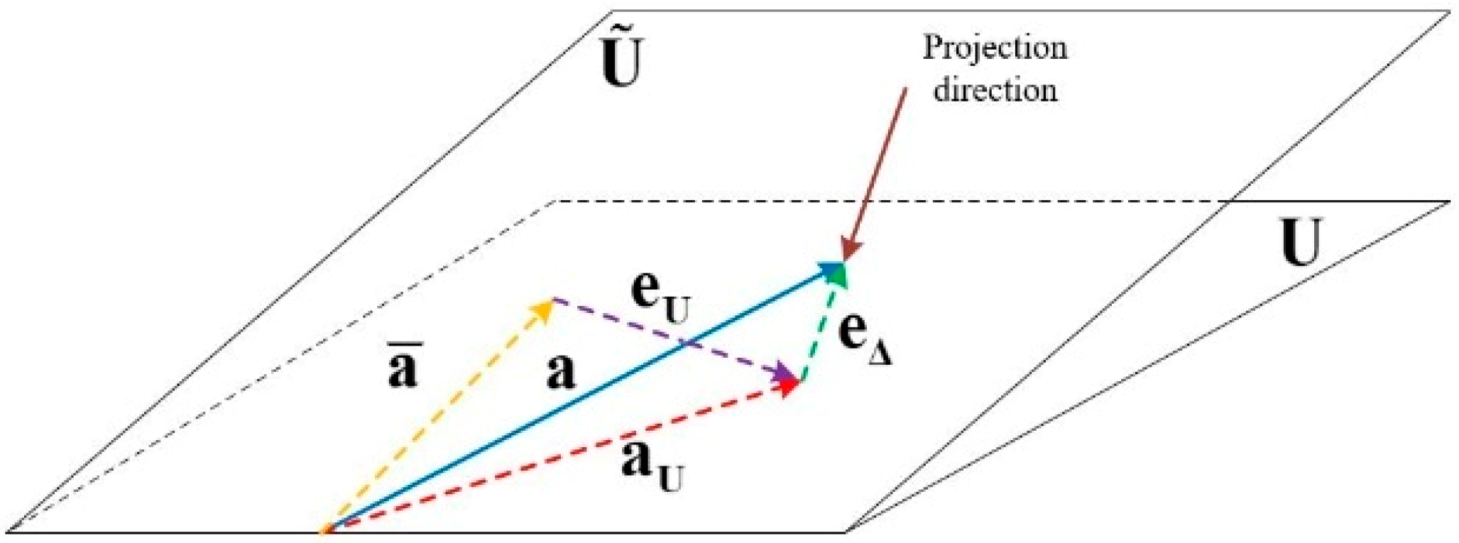
3.1. Actual Steering Vector Decomposition

Theoretically, we can build a positive definite matrix $\tilde{C}={\displaystyle {\int }_{\mathrm{\Theta }}a(\theta )}{a}^H(\theta )d\theta$ and obtain a subspace $\tilde{U}$ spanned by the principal eigenvectors ${\left\{{\tilde{u}}_m\right\}}_{m=1}^L$ of $\tilde{C}$ corresponding to the $L$ largest eigenvalues:

$$\tilde{U}=[{\tilde{u}}_1,{\tilde{u}}_2,\cdots ,{\tilde{u}}_L]$$

(15)

Here, $a(\theta )$ denotes the actual steering vector whose DOA is $\mathrm{\Theta }$. Since the $L$ largest eigenvalues contain most of the energy of the eigenvalues, any actual steering vector $\left\{a(\theta )|\theta \in \mathrm{\Theta }\right\}$ is believed to lie within the subspace $\tilde{U}$. Hence, the actual steering vector can be expressed as a linear combination of the columns of $\tilde{U}$:

$$a=\tilde{U}r$$

(16)

where $r$ is the coefficient vector. In fact, $\tilde{U}$ is unavailable in practice due to the imperfect knowledge of the actual steering vector. Instead, we build another subspace $U$ spanned by the set of presumed steering vectors $\left\{\overline{a}(\theta )|\theta \in \mathrm{\Theta }\right\}$:

$$U=[u_1,u_2,\cdots ,u_L]$$

(17)

where ${\left\{{\tilde{u}}_m\right\}}_{m=1}^L$ denotes the $L$ principal eigenvectors of $C={\displaystyle {\int }_{\mathrm{\Theta }}\overline{a}(\theta ){\overline{a}}^H(\theta )d\theta }$. It can be easily seen that the matrix $C$ will deviate from the matrix $\tilde{C}$ when steering vector errors occur, leading to a mismatch between the subspaces $\tilde{U}$ and $U$:

$$\tilde{U}=U+{\Delta }_U$$

(18)

where ${\Delta }_U$ is the $M\times L$ mismatch matrix. By substituting Problem (18) into Problem (16), $a$ can be decomposed into two components, i.e.:

$$a=a_U+e_{\Delta }$$

(19)

Here, we define $a_U\triangleq Ur$ and $e_{\Delta }\triangleq {\Delta }_{U}r$. It can be seen that $a_U$ is a vector lying within the subspace $U$ and $e_{\Delta }$ is an error vector caused by ${\Delta }_U$. It is worth mentioning that in the case of only DOA mismatch, we have $U=\tilde{U}$, as long as $\mathrm{\Theta }$ contains the actual DOA of the SOI and avoids all the interferences. In other words, the existence of DOA mismatch will not result in the mismatch between $U$ and $\tilde{U}$. Consequently, the error vector $e_U\triangleq a_U-\overline{a}$, which also lies within $U$, is dominated by DOA mismatch while the error vector $e_{\Delta }$ is dominated by other array imperfections. Here, the presumed steering vector $\overline{a}$ is an arbitrary element in the set of $\left\{\overline{a}(\theta )|\theta \in \mathrm{\Theta }\right\}$.

The relationship among $\tilde{U}$, $U$, $e_U$, $e_{\Delta }$, $\overline{a}$, $a_U$, and $a$ is depicted geometrically in Figure 2. As shown, $a_U$ can be considered as the oblique projection vector of the actual steering vector $a$ onto the subspace $U$ and the projection direction is opposite to the direction of the error vector $e_{\Delta }$. The basic idea behind our approach is to estimate the actual steering vector $a$ in two steps. We first search for the oblique projection steering vector $a_U$ within the subspace $U$ and then search for the actual steering vector $a$ within the neighborhood of $a_U$. In the following subsections, different optimization principles are utilized to estimate the oblique projection steering vector and the actual steering vector, respectively.

3.2. Oblique Projection Steering Vector Estimation

Since $a_U$ lies within the subspace $U$, it can be expressed as the linear combination of the columns of $U$:

$$a_U={\alpha }_1{u}_1+{\alpha }_2{u}_2+\cdots +{\alpha }_L{u}_L$$

(20)

By multiplying $u_k^H(k=1,\cdots ,L)$ on both sides of (20), we can easily obtain the coefficients ${\alpha }_k=u_k^H{a}_U(k=1,2,\cdots ,L)$. Then, Problem (20) can be rewritten as:

$$a_U=U{U}^H{a}_U$$

(21)

By making use of Problem (21), the oblique projection $a_U$ can be forced to belong to the subspace $U$. Additionally, an equality constraint $\Vert a_U\Vert =\sqrt{M}$, which maintains the norm of the estimated $a_U$, is imposed to avoid the scaling ambiguity. Now we can search for $a_U$ by maximizing the output power $1/a_U^H{\widehat{R}}_x^{-1}{a}_U$, which can be formulated as the following optimization problem:

$$\begin{array}{cc}\hfill \underset{a_U}{\min }& a_U^H{\widehat{R}}_x^{-1}{a}_U\hfill \\ \hfill \mathrm{subject}\mathrm{to}& a_U=U{U}^H{a}_U\hfill \\ \hfill & \Vert a_U\Vert =\sqrt{M}\hfill \end{array}$$

(22)

By substituting the equality constraint $a_U=U{U}^H{a}_U$ into the objective function, Problem (22) can be modified as:

$$\begin{array}{cc}\hfill \underset{a_U}{\min }& a_U^{H}U{U}^H{\widehat{R}}_x^{-1}U{U}^H{a}_U\hfill \\ \hfill \mathrm{subject}\mathrm{to}& \Vert a_U\Vert =\sqrt{M}\hfill \end{array}$$

(23)

It is worth noting that the solution to Problem (23) may result in the magnification of output noise especially at low SNR, thus an extra constraint $\left|a_U^H\overline{a}(\theta )\right|\le \left|{\overline{a}}^H\overline{a}(\theta )\right|$ for any $\theta \in \overline{\mathrm{\Theta }}$ is invoked to control the power from the sidelobe region $\overline{\mathrm{\Theta }}$. This constraint can be equivalently expressed as $a_U^H\overline{C}{a}_U\le {\overline{a}}^H\overline{C}\overline{a}$, where $\overline{C}={\displaystyle {\int }_{\overline{\mathrm{\Theta }}}\overline{a}(\theta ){\overline{a}}^H(\theta )}d\theta$ [13]. Now, the estimation problem can be written as:

$$\begin{array}{cc}\hfill \underset{a_U}{\min }& a_U^{H}U{U}^H{\widehat{R}}_x^{-1}U{U}^H{a}_U\hfill \\ \hfill \mathrm{subject}\mathrm{to}& a_U^H\overline{C}{a}_U\le {\overline{a}}^H\overline{C}\overline{a}\hfill \\ \hfill & \Vert a_U\Vert =\sqrt{M}\hfill \end{array}$$

(24)

It is interesting that the steering vector estimation problem in Reference [17] has some insightful connections to Problem (24). Since the approach in Reference [17] only considers the factor of DOA mismatch, the actual steering vector is represented as $a=Ur$ directly, where $r$ denotes the coefficient vector. The origin estimation problem in Reference [17] can be expressed in terms of $r$ as:

$$\begin{array}{cc}\hfill \underset{r}{\min }& r^H{U}^H{\widehat{R}}_x^{-1}Ur\hfill \\ \hfill \mathrm{subject}\mathrm{to}& \Vert r\Vert =\sqrt{M}\hfill \end{array}$$

(25)

Using Problem (21), we can easily obtain $r=U^{H}a$ and then Problem (25) can be equivalently rewritten as (23). As we discussed above, an extra sidelobe control constraint is introduced in Problem (24) as compared with Problem (23). Consequently, it is expected that the proposed method can provide better performance than the beamformer in Reference [17] in the case of large DOA mismatch, especially in the low SNR region.

Unfortunately, the QCQP Problem (24) is a nonconvex NP-hard problem because of the equality constraint. Next, we focus on solving Problem (24) in polynomial time. Using the equalities $a_U^{H}U{U}^H{\widehat{R}}_x^{-1}U{U}^H{a}_U=tr(U{U}^H{\widehat{R}}_x^{-1}U{U}^H{a}_U{a}_U^H)$, $a_U^H\overline{C}{a}_U=tr(\overline{C}{a}_U{a}_U^H)$, and $a_U^H{a}_U=tr(a_U{a}_U^H)$, where $tr(·)$ represents the trace of a matrix, Problem (24) can be equivalently written as:

$$\begin{array}{cc}\hfill \underset{a_U}{\min }& tr(U{U}^H{\widehat{R}}_x^{-1}U{U}^H{a}_U{a}_U^H)\hfill \\ \hfill \mathrm{subject}\mathrm{to}& tr(\overline{C}{a}_U{a}_U^H)\le {\overline{a}}^H\overline{C}\overline{a}\hfill \\ \hfill & tr(a_U{a}_U^H)=M\hfill \end{array}$$

(26)

By introducing the positive semidefinite matrix variable $Q\triangleq a_U{a}_U^H$ and using the semidefinite relaxation technique [20], we obtain the following relaxed problem:

$$\begin{array}{cc}\hfill \underset{Q}{\min }& tr(R_{0}Q)\hfill \\ \hfill \mathrm{subject}\mathrm{to}& tr(R_{1}Q)\le \beta \hfill \\ \hfill & tr(R_{2}Q)=M\hfill \\ \hfill & Q\ge 0\hfill \end{array}$$

(27)

where $R_0\triangleq U{U}^H{\widehat{R}}_x^{-1}U{U}^H$, $R_1\triangleq \overline{C}$, $R_2\triangleq I_M$,$\beta \triangleq {\overline{a}}^H\overline{C}\overline{a}$. Note that we drop the nonconvex rank-one constraint on $Q$ and just require $Q\ge 0$. Problem (27) is a convex semidefinite program (SDP) problem and can be easily solved. Generally, the solution to the SDP problem may not be exactly rank-one. Thus, we first check the rank of the optimal solution $Q^{\ast }$. If $rank(Q^{\ast })=1$, then we can easily write $Q^{\ast }=a_U^{\ast }{a}_U^{\ast H}$ by eigen-decomposition and $a_U^{\ast }$ will be the optimal solution to (24). If $rank(Q^{\ast })\ge 2$, then we can adopt the rank-one decomposition theorem [22] to find a rank-one optimal solution $a_U^{\ast }{a}_U^{\ast H}$ to Problem (27), and $a_U^{\ast }$ is optimal for Problem (24). The rank-one decomposition theorem [22] is cited as the following lemma.

Lemma 1.

Let$A_i(i=0,1,2)$be$M\times M(M\ge 3)$complex Hermitian matrices, and$X$be a nonzero Hermitian positive semidefinite matrix with rank$r$.

If$r\ge 3$, then one can find a nonzero vector$y\in \mathrm{Range}(X)$(synthetically denoted as$y=D_1(X,A_0,A_1,A_2)$), such that:

$$tr(A_{i}y{y}^H)=tr(A_{i}X),i=0,1,2$$

(28)

If$r=2$, then for any$z\notin \mathrm{Range}(X)$, one can find a nonzero vector$y\in {ℂ}^M$in the linear subspace spanned by$z$and$\mathrm{Range}(X)$(synthetically denoted as$y=D_2(X,A_0,A_1,A_2)$), such that:

$$tr(A_{i}y{y}^H)=tr(A_{i}X),i=0,1,2$$

(29)

It follows from Lemma 1 that if $rank(Q^{\ast })\ge 2$, we can find a vector $a_U^{\ast }$ such that:

$$tr(R_i{a}_U^{\ast }{a}_U^{\ast H})=tr(R_i{Q}^{\ast }),i=0,1,2$$

(30)

Hence, $a_U^{\ast }{a}_U^{\ast H}$ satisfies all the constraints in Problem (27) and the objective function evaluated at $a_U^{\ast }$ is equal to the optimal value of Problem (27); as a consequence, $a_U^{\ast }{a}_U^{\ast H}$ is optimal for Problem (27) and $a_U^{\ast }$ is an optimal solution to Problem (24). The procedure to find the optimal solution $a_U^{\ast }$ is summarized in Algorithm 1.

Algorithm 1. Procedure leading to an optimal solution to (24)

Input: ${\widehat{R}}_x$, $\overline{a}$, $U$ and $\overline{C}$ Output: An optimal solution $a_U^{\ast }$ to (24) 1: solve the SDP problem (27) and find an optimal solution $Q^{\ast }$. 2: if $rank(Q^{\ast })=1$, then 3: find the optimal solution $a_U^{\ast }$ via eigen-decomposition, i.e., $Q^{\ast }=a_U^{\ast }{a}_U^{\ast H}$ 4: else if $rank(Q^{\ast })=2$, then 5: find $a_U^{\ast }=D_2(Q^{\ast },R_0,R_1,R_2)$ 6: else, then 7: find $a_U^{\ast }=D_1(Q^{\ast },R_0,R_1,R_2)$ 8: end if 9: return $a_U^{\ast }$

3.3. Actual Steering Vector Estimation

Besides the DOA mismatch, the Capon beamformer is also very sensitive to other array imperfections, which contributes to the error vector $e_{\Delta }$ as shown in Figure 2. Based on this fact, we impose a bounded-norm constraint on the error vector $e_{\Delta }$ and assume that the actual steering vector $a$ lies in a spherical uncertainty set $S_a$:

$$a\in S_a\triangleq \left\{a|\Vert a-a_U\Vert \le \gamma \right\}$$

(31)

where $\gamma >0$ is a given constant. In the following derivations, we design a novel objective function to search for the actual steering vector in $S_a$. Essentially, the novel objective function is based on maximizing the output SINR. Based on the introduced array signal model, the output SINR (3) can be reformulated as follows:

$$\begin{array}{cc}\hfill {\mathrm{SINR}}_{\mathrm{out}}& =\frac{w^H{R}_{s}w}{w^H{R}_{\mathrm{int}}w+w^H{R}_{n}w}\hfill \\ & =\frac{{\sigma }_0^2{\left|w^{H}a\right|}^2}{{\displaystyle \sum _{i=1}^{D-1}{\sigma }_i^2{\left|w^H{a}_i\right|}^2+{\sigma }_n^2{w}^{H}w}}\hfill \end{array}$$

(32)

Utilizing the weight of the SCB (8), the array response of the SOI, i.e., $\left|w^{H}a\right|$, is 1, and the array response of the interference can be obtained by:

$$\begin{array}{cc}\hfill H(a_i)& =\left|w^H{a}_i\right|\hfill \\ & =\frac{\left|a^H{R}_x^{-1}{a}_i\right|}{\left|a^H{R}_x^{-1}a\right|}=\frac{\left|a^{H}T{T}^H{a}_i\right|}{\left|a^{H}T{T}^{H}a\right|}\hfill \end{array}$$

(33)

where $T\triangleq R_x^{-1/2}$. Applying the Cauchy-Schwarz inequality $\left|a^{H}T{T}^H{a}_i\right|\le \Vert a^{H}T\Vert \Vert a_i^{H}T\Vert$, we can easily have that:

$$H(a_i)\le \frac{\Vert a^{H}T\Vert \Vert a_i^{H}T\Vert }{{\Vert a^{H}T\Vert }^2}=\frac{\sqrt{1/a^H{R}_x^{-1}a}}{{\sqrt{1/a_i^H{R}_x^{-1}a}}_i}$$

(34)

Moreover, the power of the SOI and the interferences can be given by:

$${\sigma }_0^2=\frac{1}{a^H{R}_x^{-1}a},{\sigma }_i^2=\frac{1}{a_i^H{R}_x^{-1}{a}_i}$$

(35)

By substituting Problem (33)–(35) into Problem (32), we can write that:

$$\begin{array}{cc}\hfill {\mathrm{SINR}}_{\mathrm{out}}& \ge \frac{\frac{1}{a^H{R}_x^{-1}a}}{\frac{D-1}{a^H{R}_x^{-1}a}+{\sigma }_n^2\frac{a^H{R}_x^{-2}a}{{\left(a^H{R}_x^{-1}a\right)}^2}}\hfill \\ & =\frac{1}{D-1+{\sigma }_n^2\frac{a^H{R}_x^{-2}a}{a^H{R}_x^{-1}a}}\hfill \end{array}$$

(36)

Hence, the maximization of the output SINR is equivalent to:

$$\underset{a}{\max }\frac{a^H{R}_x^{-1}a}{a^H{R}_x^{-2}a}$$

(37)

Using the sample covariance matrix ${\widehat{R}}_x^{-1}$, the following optimization problem is constructed to search for the actual steering vector of the SOI in the uncertainty set:

$$\begin{array}{cc}\hfill \underset{a}{\max }& \frac{a^H{\widehat{R}}_x^{-1}a}{a^H{\widehat{R}}_x^{-2}a}\hfill \\ \hfill \mathrm{subject}\mathrm{to}& \Vert a-a_U\Vert \le \gamma \hfill \end{array}$$

(38)

Problem (38) is a nonconvex fractional quadratic optimization problem. With an extra variable $t(t^2=1)$, it can be transformed into a homogeneous form:

$$\begin{array}{cc}\hfill \underset{g}{\max }& \frac{tr(P_{0}g{g}^H)}{tr(P_{1}g{g}^H)}\hfill \\ \hfill \mathrm{subject}\mathrm{to}& tr(P_{2}g{g}^H)\le {\gamma }^2\hfill \\ \hfill & tr(P_{3}g{g}^H)=1\hfill \end{array}$$

(39)

where $g\triangleq \left[\begin{array}{l}a\\ t\end{array}\right]$, $P_0\triangleq \left[\begin{array}{l}{\widehat{R}}_x^{-1}{0}_{M\times 1}\\ 0_{1\times M}0\end{array}\right]$, $P_1\triangleq \left[\begin{array}{l}{\widehat{R}}_x^{-2}{0}_{M\times 1}\\ 0_{1\times M}0\end{array}\right]$, $P_2\triangleq \left[\begin{array}{cc}{I}_M\hfill & -a_U\hfill \\ -a_U^H\hfill & a_U^H{a}_U\hfill \end{array}\right]$, $P_3\triangleq \left[\begin{array}{l}{0}_{M\times M}{0}_{M\times 1}\\ 0_{1\times M}1\end{array}\right]$. We highlight that Problem (38) and Problem (39) have equal optimal values and their optimal solutions differ from one to another by $t$, i.e., $a^{\ast }=g^{\ast }/t$. Next, we define the positive semidefinite matrix variable $G\triangleq g{g}^H$ and drop the rank-one constraint on $G$ by applying the semidefinite relaxation technique [20]. Then, the following relaxed problem can be obtained:

$$\begin{array}{cc}\hfill \underset{G}{\max }& \frac{tr(P_{0}G)}{tr(P_{1}G)}\hfill \\ \hfill \mathrm{subject}\mathrm{to}& tr(P_{2}G)\le {\gamma }^2\hfill \\ \hfill & tr(P_{3}G)=1\hfill \\ \hfill & G\ge 0\hfill \end{array}$$

(40)

It is worth mentioning that problem (40) is a quasi-convex problem due to the linear fractional structure of the objective function. Here, the Charnes-Cooper transformation technique [21] is exploited in order to transform Problem (40) into a convex SDP problem. We define the transformed variable $W\triangleq \eta G$, where $\eta \ge 0$ complies with $tr(P_{1}W)=1$, and consider the following convex SDP problem:

$$\begin{array}{cc}\hfill \underset{W,\eta }{\max }& tr(P_{0}W)\hfill \\ \hfill \mathrm{subject}\mathrm{to}& tr(P_{1}W)=1\hfill \\ \hfill & tr(P_{2}W)\le \eta {\gamma }^2\hfill \\ \hfill & tr(P_{3}W)=\eta \hfill \\ \hfill & W\ge 0,\eta \ge 0\hfill \end{array}$$

(41)

Based on Lemma 3.3 in [21], problem (40) is equivalent to (41) in the sense that they have equal optimal values and their optimal solutions differ from one to another by a constant ${\eta }^{\ast }$. In other words, once an optimal solution $\left(W^{\ast },{\eta }^{\ast }\right)$ to (41) is obtained, the optimal solution to Problem (40) can be easily obtained by $G^{\ast }=W^{\ast }/{\eta }^{\ast }$. Next, we focus on finding an optimal solution to Problem (39) with $G^{\ast }$. First, we check the rank of $G^{\ast }$. If $G^{\ast }=g^{\ast }{g}^{\ast }{}^H$ is rank-one, then $g^{\ast }$ will be the optimal solution to Problem (39). If $rank(G^{\ast })\ge 2$, then there exists a vector $g^{\ast }$ based on Lemma 1 such that:

$$\{\begin{array}{l}tr((P_0-v^{\ast }{P}_1)g^{\ast }{g}^{\ast }{}^H)=tr((P_0-v^{\ast }{P}_1)G^{\ast })=0\\ tr(P_i{g}^{\ast }{g}^{\ast }{}^H)=tr(P_i{G}^{\ast }),i=2,3\end{array}$$

(42)

Here, $v^{\ast }=tr(P_0{G}^{\ast }{}^H)/tr(P_1{G}^{\ast }{}^H)$ denotes the optimal value of Problem (40). As shown in Problem (42), $g^{\ast }{g}^{\ast }{}^H$ is feasible to Problem (40) and the objective function evaluated at $g^{\ast }$, i.e., $tr(P_0{g}^{\ast }{g}^{\ast H})/tr(P_1{g}^{\ast }{g}^{\ast H})$, is equal to the optimal value $v^{\ast }$; thus, $g^{\ast }{g}^{\ast }{}^H$ is optimal for Problem (40) and $g^{\ast }$ is the optimal solution to Problem (39). Then, the optimal solution to Problem (38) can be easily obtained by $a^{\ast }=g^{\ast }/t$. Algorithm 2 summarizes the procedure to find an optimal solution $a^{\ast }$.

Algorithm 2. Procedure leading to an optimal solution to (38)

Input: ${\widehat{R}}_x$, $a_U^{\ast }$ and $\gamma$ Output: An optimal solution $a^{\ast }$ to (38) 1: solve the SDP problem (41), find an optimal solution $(W^{\ast },{\eta }^{\ast })$ and the optimal value $v^{\ast }$. 2: let $G^{\ast }=W^{\ast }/{\eta }^{\ast }$ 3: if $rank(G^{\ast })=1$, then 4: perform an eigen-decomposition, $G^{\ast }=g^{\ast }{g}^{\ast H}$ 5: else if $rank(G^{\ast })=2$, then 6: find $g^{\ast }=D_2(G^{\ast },P_0-v^{\ast }{P}_1,P_2,P_3)$ 7: else, then 8: find $g^{\ast }=D_1(G^{\ast },P_0-v^{\ast }{P}_1,P_2,P_3)$ 9: end if 10: return $a^{\ast }=g^{\ast }/t$

Finally, in order to avoid the ambiguity, the norm of the estimated actual steering vector $a^{\ast }$ should be scaled back to $\sqrt{M}$:

$$a^{\ast }:=\frac{\sqrt{M}}{\Vert a^{\ast }\Vert }{a}^{\ast }$$

(43)

3.4. Proposed Robust Capon Beamformer

With the estimated actual steering vector $a^{\ast }$, the weight of the proposed robust Capon beamformer can be formulated as:

$$w=\frac{{\widehat{R}}_x^{-1}{a}^{\ast }}{a^{\ast H}{\widehat{R}}_x^{-1}{a}^{\ast }}$$

(44)

The proposed robust Capon beamforming algorithm is summarized in

Table 1. Proposed robust Capon beamforming algorithm.

1. Calculate the sample covariance matrix ${\widehat{R}}_x$ as (9) 2. Estimate the actual steering vector $a^{\ast }$ in two steps: Step 1: Estimate the oblique projection steering vector $a_U^{\ast }$ via Algorithm 1 Step 2: Estimate the actual steering vector $a^{\ast }$ via Algorithm 2 and normalize it as (43) 3. Calculate the weight $w$ based on ${\widehat{R}}_x$ and $a^{\ast }$ as (44)

. In the proposed method, the main computational complexity lies in the solution to the SDP Problem (27) and Problem (41), which requires a complexity cost of $O(M^{4.5}\log (1/\delta ))$ with $\delta$ representing a prescribed accuracy [20], and both the specific rank-one decomposition and the matrix inversion operation require a computational complexity of $O(M^3)$. Consequently, the algorithm complexity of the proposed method is $O(\max (M^{4.5}\log (1/\delta ),M^3))$.

4. Simulations

In the simulations, we assume a uniform linear sonar array (ULA) of 10 omnidirectional elements spaced half a wavelength apart receiving three Gaussian sources: the SOI from a direction ${\theta }_0\in \mathrm{\Theta }$ and two interferences from $\left\{{\theta }_1=-{40}^{\circ },{\theta }_2={50}^{\circ }\right\}$. The interference-to-noise ratio (INR) is fixed at 40 dB. The presumed look direction is fixed at $0^{\circ }$. In addition to DOA mismatch, the array element calibration error and position error are also considered in all simulations. The element calibration error is caused by gain and phase perturbations, which are assumed to be uniformly distributed in [0.8,1.2] and $[-\pi /100,\pi /100]$, respectively. The element position error is assumed to be drawn uniformly from the interval [−0.05,0.05] measured in wavelength. Simulation results are averaged based on 1000 Monte-Carlo runs. The array element calibration error and position error change from run to run but keep fixed from snapshot to snapshot.

The proposed beamformer is compared with the SCB and robust approaches including the ESB [12], the Worst-Case beamformer [9], Zhuang’s beamformer [16], Zhang’s beamformer [17], and Wen’s beamformer [18]. In Zhuang’s, Zhang’s, Wen’s and the proposed beamformer, the ROI $\mathrm{\Theta }$ is set to be $[-{10}^{\circ },{10}^{\circ }]$. Six principal eigenvectors of $C={\displaystyle {\int }_{\mathrm{\Theta }}\overline{a}(\theta ){\overline{a}}^H(\theta )}d\theta$, whose corresponding eigenvalues contain 99.99% of the sum of all eigenvalues, are used to form the subspace $U$. The values of the uncertainty level for the Worst-Case beamformer and Wen’s beamformer are set to be $\epsilon =3$ and $\beta =2$, respectively. Two cases with $\xi =3$ and $\xi =4$ are considered in the ESB and Zhuang’s beamformer, where $\xi$ is the estimated number of sources. The parameter $\gamma =1.5$ is used for the proposed beamformer. CVX MATLAB toolbox [23] is used for solving the optimization problems in the Worst-Case beamformer and the proposed method.

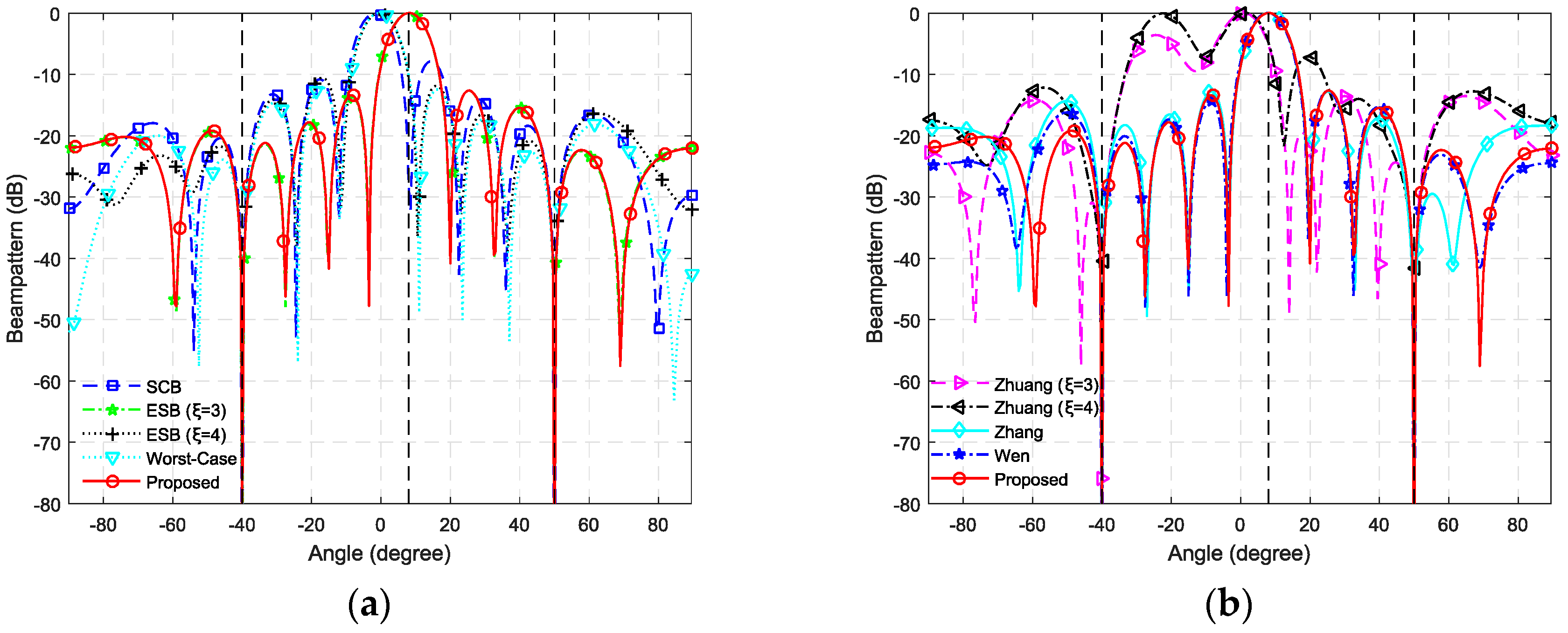
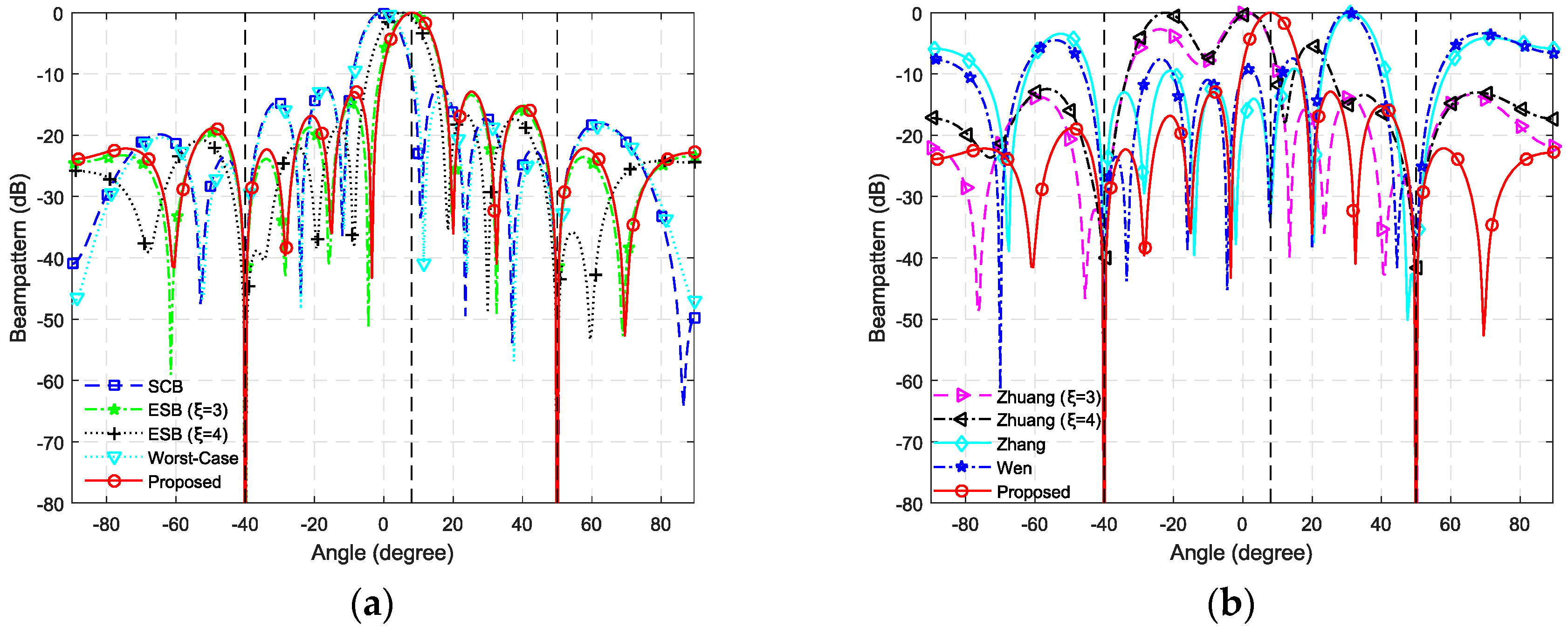
4.1. Beampatterns

In the first simulation, we consider the resultant beampatterns of these beamformers. The actual DOA of the SOI is assumed to be ${\theta }_0=8^{\circ }$, that is to say, the DOA mismatch is $8^{\circ }$ in this example. The number of snapshots $N=500$ is taken. Figure 3 and Figure 4 show the resultant beampatterns for SNR = 0 dB and SNR = −15 dB, respectively. The black dashed lines in Figure 3 and Figure 4 represent the actual DOAs of the SOI and interferences. As shown, all these beamformers have deep nulls at the directions of interferences but only the ESB of $\xi =3$ and the proposed method point their mainlobes towards the actual DOA of SOI in both SNR cases. The SCB, the Worst-Case beamformer and Zhuang’s beamformer point their mainlobes towards the presumed look direction rather than the actual DOA of the SOI, and the SCB suffers from the problem of signal self-nulling when SNR = 0 dB, because the SOI is considered as an interference. The ESB of $\xi =4$ also does not work well when SNR = 0 dB. Zhang’s beamformer and Wen’s beamformer fail to maintain the distortionless response towards the actual DOA of SOI when SNR = −15 dB.

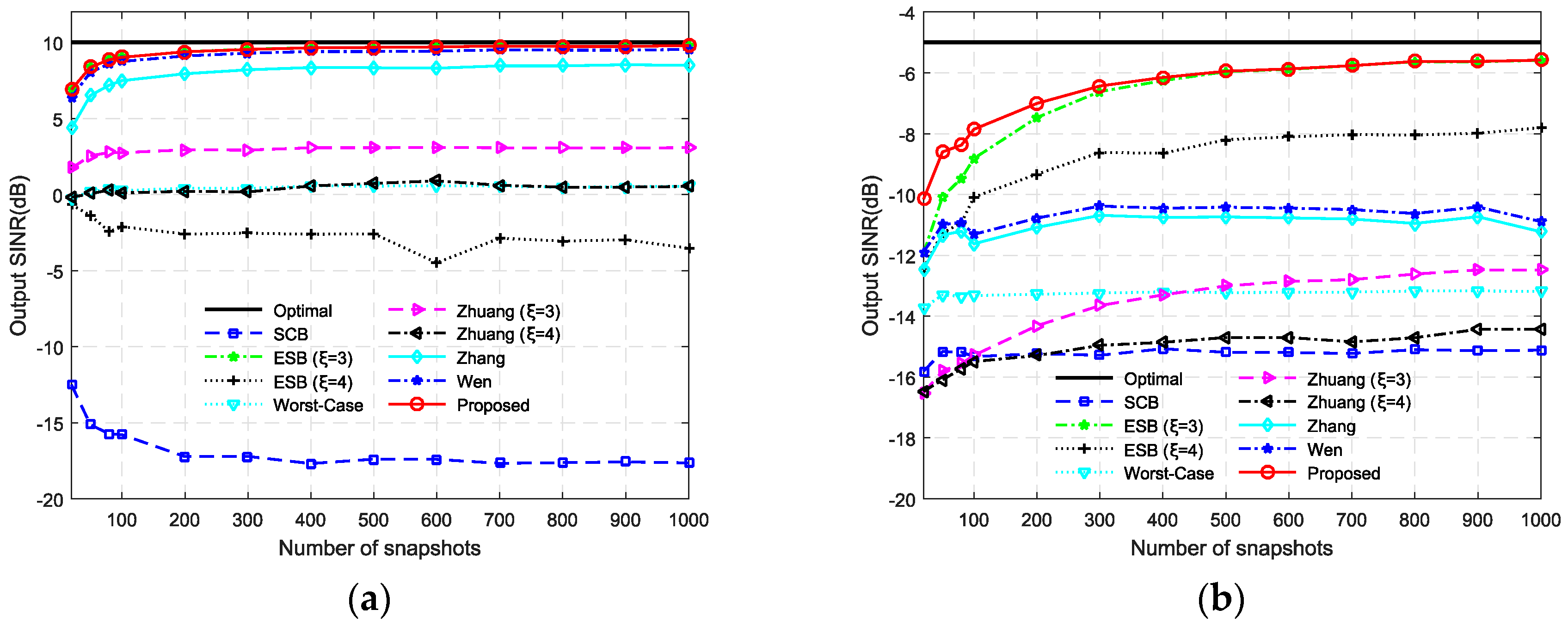
4.2. Output SINR versus Number of Snapshots

The second simulation aims to investigate the effect of the number of snapshots on the output SINR. We vary the number of snapshots from 20 to 1000 while the parameters of the SOI are kept unchanged. The output SINR versus the number of snapshots for SNR = 0 dB and SNR = −15 dB are shown in Figure 5a,b, respectively. In the figures, the black bold lines denote the optimal SINR. One can observe that the output SINR of the SCB, the Worst-Case beamformer and Zhuang’s beamformer degrade significantly with a DOA mismatch of $8^{\circ }$. Zhang’s beamformer and Wen’s beamformer can provide sufficient robustness when SNR = 0 dB; however, their performances suffer from severe degradation when SNR = −15 dB. The ESB achieves high output SINR in both SNR cases, but it suffers from the overestimated number of sources. The proposed method achieves the best performance among all these beamformers.

4.3. Output SINR versus Input SNR

Next, we vary the input SNR in order to investigate the effect of input SNR on the performance of these beamformers. Other parameters remain the same as the first example. Figure 6 compares the output SINR of the tested beamformers and the optimal SINR is denoted by the black bold line. The results indicate that the ESB of $\xi =3$ and the proposed beamformer achieve the best performance among these beamformers. The SCB, the ESB of $\xi =4$, the Worst-Case beamformer and Zhuang’s beamformer do not work well with a large DOA mismatch. The performance of Zhang’s beamformer degrades in the high SNR region. This is because it is sensitive to other array imperfections and the effects caused by the sensitivity will be enhanced when SNR is larger. Moreover, it also suffers from severe performance degradation in the low SNR region. Wen’s beamformer has good performance in the high SNR region; however, its performance in the low SNR region is much worse than the proposed method.

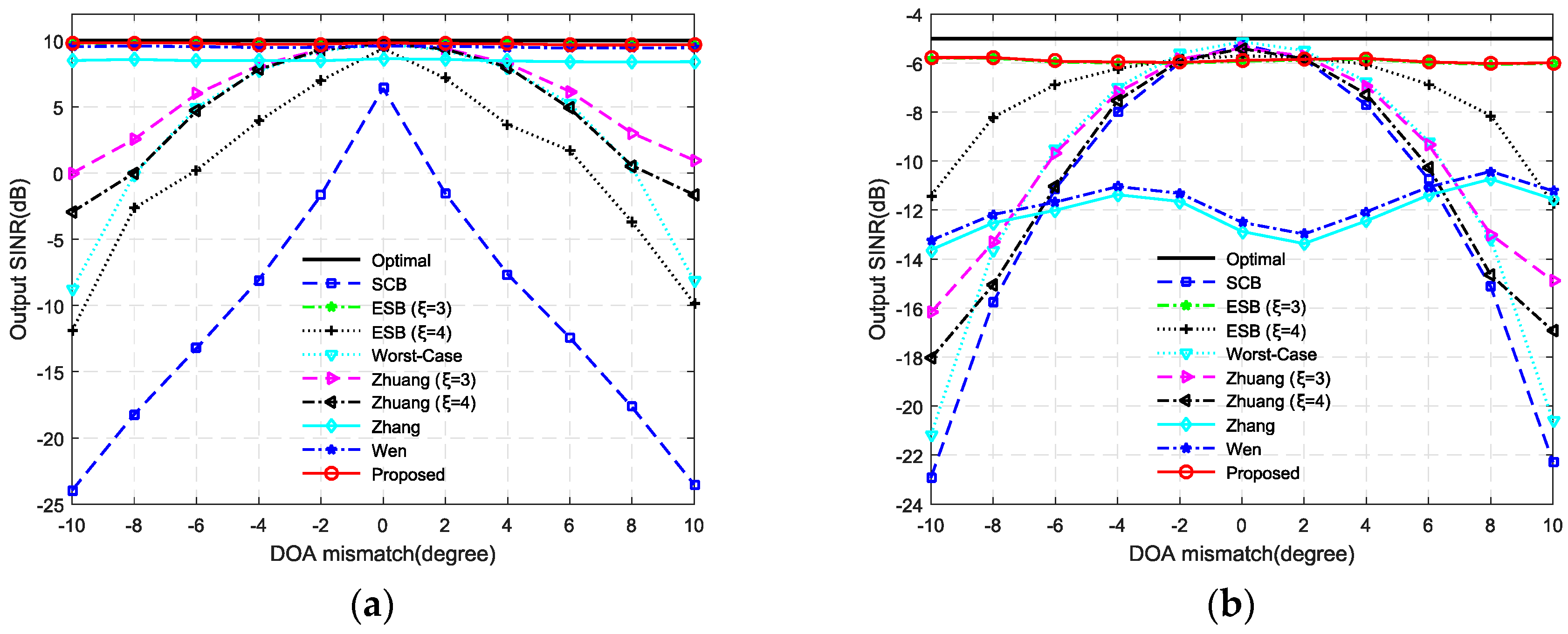
4.4. Output SINR versus DOA Mismatch

In this simulation, we generally adopt the parameter setting in the first simulation and vary the DOA of SOI from $-{10}^{\circ }$ to ${10}^{\circ }$. That is, the DOA mismatch varies from $-{10}^{\circ }$ to ${10}^{\circ }$. The results for SNR = 0 dB are depicted in Figure 7a, and the results for SNR = −15 dB are depicted in Figure 7b. The corresponding optimal SINRs at SNR = 0 dB and SNR = −15 dB are represented by the black bold lines. It is clearly illustrated that the ESB of $\xi =3$ and the proposed method outperform the other beamformers. While Zhang’s beamformer and Wen’s beamformer have sufficient capacity to provide robustness against large DOA mismatch when SNR = 0 dB, their performances degrade severely when SNR = −15 dB. The SCB is very sensitive to the DOA mismatch and it is more sensitive when the SNR is larger. The Worst-Case beamformer, the ESB of $\xi =4$ and Zhuang’s beamformer cannot provide robustness against a large DOA mismatch.

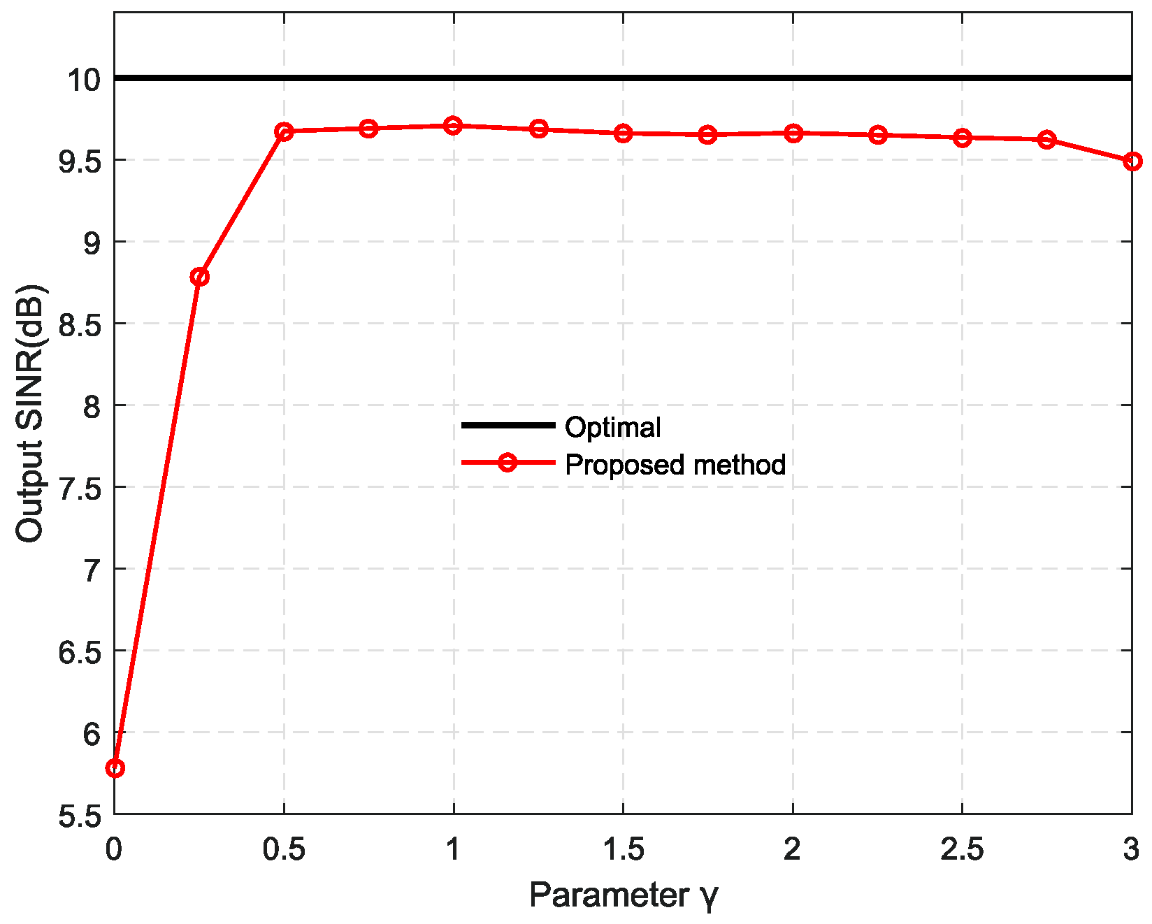
4.5. Output SINR versus Parameter $\gamma$

Lastly, the effect of the parameter $\gamma$ on the proposed robust Capon beamformer is considered. The SNR is fixed at 0 dB and other parameters are kept unchanged as the first simulation. Figure 8 shows the output SINR versus the parameter $\gamma$ and the black bold line stands for the optimal SINR. One can observe that the performance of the proposed method remains steady and close to the optimal value in the range of $0.5\le \gamma \le 3$. This implies that the performance of the proposed method is insensitive to the choice of the parameter $\gamma$, and thus we can set $\gamma$ in a relaxed way.

From the above simulation results, it is clear that ESB and the proposed method have superior performance on SINR improvement. The computational complexity of the ESB is $O(M^3)$, which is lower than that of the proposed beamformer. However, in comparison with the ESB which requires an accurate number of sources, the proposed beamformer only requires a relaxed parameter setting. Therefore, the proposed method is more suitable for practical applications of passive sonar systems.

5. Conclusions

A new robust Capon beamformer has been proposed in order to improve the robustness against the steering vector error dominated by large DOA mismatch for passive sonar. The proposed technique decomposes the actual steering vector into two components by projecting it obliquely onto a subspace. Based on this, the oblique projection steering vector is estimated within the subspace and then the actual steering vector is estimated within the neighborhood of the oblique projection steering vector. Nonconvex formulations for the two estimation problems have been solved by semidefinite relaxation, Charnes-Cooper transformation and rank-one decomposition theorem. The proposed beamformer can provide superior performance as compared with existing robust beamformers and only requires a relaxed parameter setting. Simulation results have been presented to demonstrate the effectiveness of the proposed beamformer in different hypothetical scenarios.

References

- Capon, J. High-resolution frequency-wavenumber spectrum analysis. Proc. IEEE 1969, 57, 1408–1418. [Google Scholar] [CrossRef]
- Van Trees, H.L. Optimum Array Processing: Part IV of Detection, Estimation, and Modulation Theory; Wiley: New York, NY, USA, 2002; pp. 443–452. [Google Scholar]
- Somasundaram, S.D.; Parsons, N.H. Evaluation of robust Capon beamforming for passive sonar. IEEE J. Ocean. Eng. 2011, 36, 686–695. [Google Scholar] [CrossRef]
- Somasundaram, S.D.; Butt, N.R.; Jakobsson, A.; Hart, L. Low complexity uncertainty-set-based robust adaptive beamforming for passive sonar. IEEE J. Ocean. Eng. 2015, 99, 1–17. [Google Scholar] [CrossRef]
- Somasundaram, S.D. Wideband robust Capon beamforming for passive sonar. IEEE J. Ocean. Eng. 2013, 38, 308–312. [Google Scholar] [CrossRef]
- Li, J.; Stoica, P.; Wang, Z.S. On robust Capon beamforming and diagonal loading. IEEE Trans. Signal Process. 2003, 51, 1702–1715. [Google Scholar]
- Li, J.; Stoica, P.; Wang, Z.S. Robust adaptive beamforming. In Robust Adaptive Beamforming; Li, J., Stoica, P., Eds.; Wiley: New York, NY, USA, 2005; Volume 3, pp. 91–93. [Google Scholar]
- Li, Y.; Ma, H.; Yu, D.; Li, C. Iterative robust Capon beamforming. Signal Process. 2016, 118, 211–220. [Google Scholar] [CrossRef]
- Vorobyov, S.A.; Gershman, A.B.; Luo, Z.Q. Robust adaptive beamforming using worst-case performance optimization: A solution to the signal mismatch problem. IEEE Trans. Signal Process. 2003, 51, 313–324. [Google Scholar] [CrossRef]
- Li, J.; Stoica, P.; Wang, Z.S. Doubly constrained robust Capon beamformer. IEEE Trans. Signal Process. 2004, 52, 2407–2423. [Google Scholar] [CrossRef]
- Beck, A.; Eldar, Y.C. Doubly constrained robust capon beamformer with ellipsoidal uncertainty sets. IEEE Trans. Signal Process. 2007, 55, 753–758. [Google Scholar] [CrossRef]
- Chang, L.; Yeh, C.C. Performance of DMI and eigenspacebased beamformers. IEEE Trans. Antennas Propag. 1992, 40, 1336–1347. [Google Scholar] [CrossRef]
- Hassanien, A.; Vorobyov, S.A.; Wong, K.M. Robust adaptive beamforming using sequential quadratic programming: An iterative solution to the mismatch problem. IEEE Signal Process. Lett. 2008, 15, 733–736. [Google Scholar] [CrossRef]
- Khabbazibasmenj, A.; Vorobyov, S.A.; Hassanien, A. Robust adaptive beamforming based on steering vector estimation with as little as possible prior information. IEEE Trans. Signal Process. 2012, 60, 2974–2987. [Google Scholar] [CrossRef]
- Fan, Z.; Liang, G. Self-steered robust adaptive beamforming. In Proceedings of the 2016 IEEE/OES China Ocean Acoustics (COA), Harbin, China, 9–11 January 2016. [Google Scholar]
- Zhuang, J.; Manikas, A. Interference cancellation beamforming robust to pointing errors. IET Signal Process. 2013, 7, 120–127. [Google Scholar] [CrossRef]
- Zhang, W.; Wang, J.; Wu, S. Robust Capon beamforming against large DOA mismatch. Signal Process. 2013, 93, 804–810. [Google Scholar] [CrossRef]
- Wen, J.; Zhou, X.; Zhang, W.; Liao, B. Robust adaptive beamforming against significant angle mismatch. In Proceedings of the 2017 IEEE Radar Conference (RadarConf), Seattle, WA, USA, 8–12 May 2017. [Google Scholar]
- Shahbazpanahi, S.; Gershman, A.B.; Luo, Z.Q.; Wong, K.M. Robust adaptive beamforming for general-rank signal models. IEEE Trans. Signal Process. 2003, 51, 2257–2269. [Google Scholar] [CrossRef]
- Luo, Z.Q.; Wong, K.M.; So, A.M.C.; Ye, Y.; Zhang, S. Semidefinite relaxation of quadratic optimization problems. IEEE Signal Process. Mag. 2010, 27, 20–34. [Google Scholar] [CrossRef]
- Mario, A.D.; Huang, Y.; Palomar, D.P.; Zhang, S.; Farina, A. Fractional QCQP with applications in ML steering direction estimation for radar detection. IEEE Trans. Signal Process. 2010, 59, 172–185. [Google Scholar]
- Ai, W.; Huang, Y.; Zhang, S. New results on Hermitian matrix rank-one decomposition. Math. Prog. 2011, 128, 253–283. [Google Scholar] [CrossRef]
- CVX: Matlab Software for Disciplined Convex Programming. Available online: http://www.standford.eud/boyd/cvx (accessed on 15 December 2018).