2.2.1. A Hybrid Graph Model of Node Distance and Number of Turns
From the perspective of energy, the transport operation cost of a transport is considered. Setting the energy consumption of a transport for a unit distance when going straight as
, and the energy consumption of a turn as
, then the objective function of the optimization model is Equation (1):
where
represents the distance traveled by the transport and
represents the number of turns of the transport.
The values of
and
can generally be determined according to the actual situation of the shipyard. However, considering that the specific measurement of the two may be difficult, the proportional relationship between the two is given:
. Therefore, the objective function of the optimization model can be rewritten as Equation (2):
where
represents how many more times energy it takes to make a turn as it takes to go straight a unit distance.
To solve this problem, it is necessary to find a method that can simultaneously present the distance relationship between nodes and the turning relationship between roads in the same graph to form a classic model in graph theory, and then use the classic shortest path algorithm to solve it.
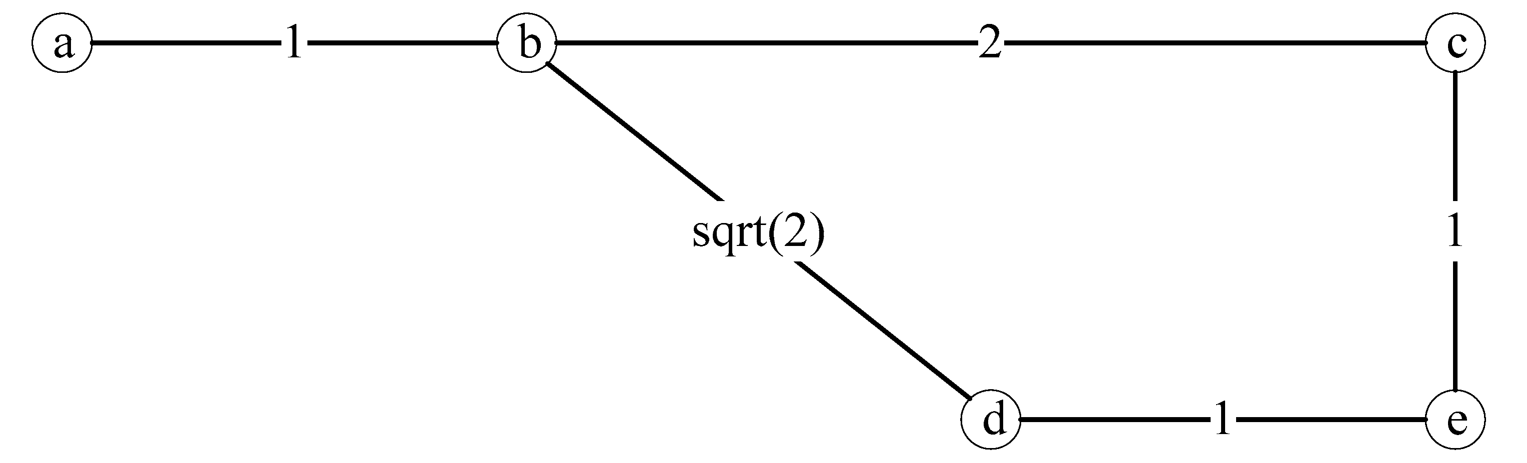
First, the modeling process of graph theory, with simple examples, is analyzed as follows. As shown in
Figure 3, suppose one wants to find an optimal path from a to e. If the shortest distance is considered only, obviously a→b→d→e is optimal, and the path length is
. However, the number of turns on this path is 2. If the path a→b→c→e is chosen, the path length is 4, and the number of turns is 1. And if
, the route a→b→c→e is optimal.
The graph shown in
Figure 3 not only reflects the distance between nodes in terms of weights, but also describes the actual location of nodes in terms of location distribution. Combining
Figure 3 as an example, the analysis describing how to combine the distance relationship and turning relationship in
Figure 3 on a new graph (
Figure 4) is as follows:
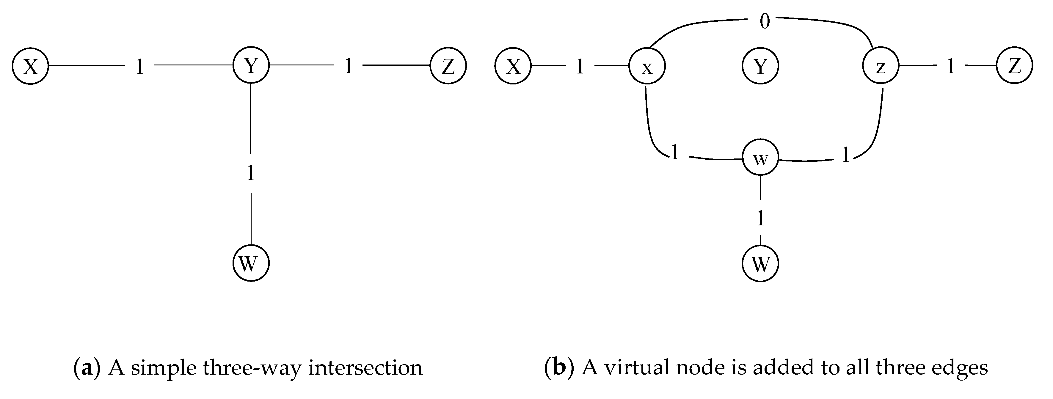
The distance between nodes is the relationship between nodes, and whether it turns or not indicates the relationship between edges connected to nodes. In order to convert the relationship between edges to the relationship between nodes, this section introduces two virtual nodes on each edge to represent the turning relationship between edges.
Figure 4a shows a simple three-way intersection. Among them, the four nodes of XYZW constitute a three-way intersection, and the distance between the nodes is all 1.
In order to be able to describe the turning relationship between the edges connected to the node Y and preserve the distance relationship between the nodes at the same time, as shown in
Figure 4b, a virtual node is added to all three edges, denoted as x, w, and z. Then the weights between the virtual nodes are used to record the turning relationship between the edges.
For example, there is no turn from XY to YZ, so the weight between xz is recorded as 0; while from XY to YW, the weight is recorded as 1. In this case, if you want to reach other paths through the Y node, you can only pass the virtual node corresponding to Y. Obviously, this completes the accumulation of the number of turns. For example, the path X→Y→Z in the original image becomes X→x→z→Z, and the sum of weights is 2+0; while in the original image, X→Y→W becomes X→x→w→W, and the sum of weights is 2+1. Therefore, such a transformation can add turning information.
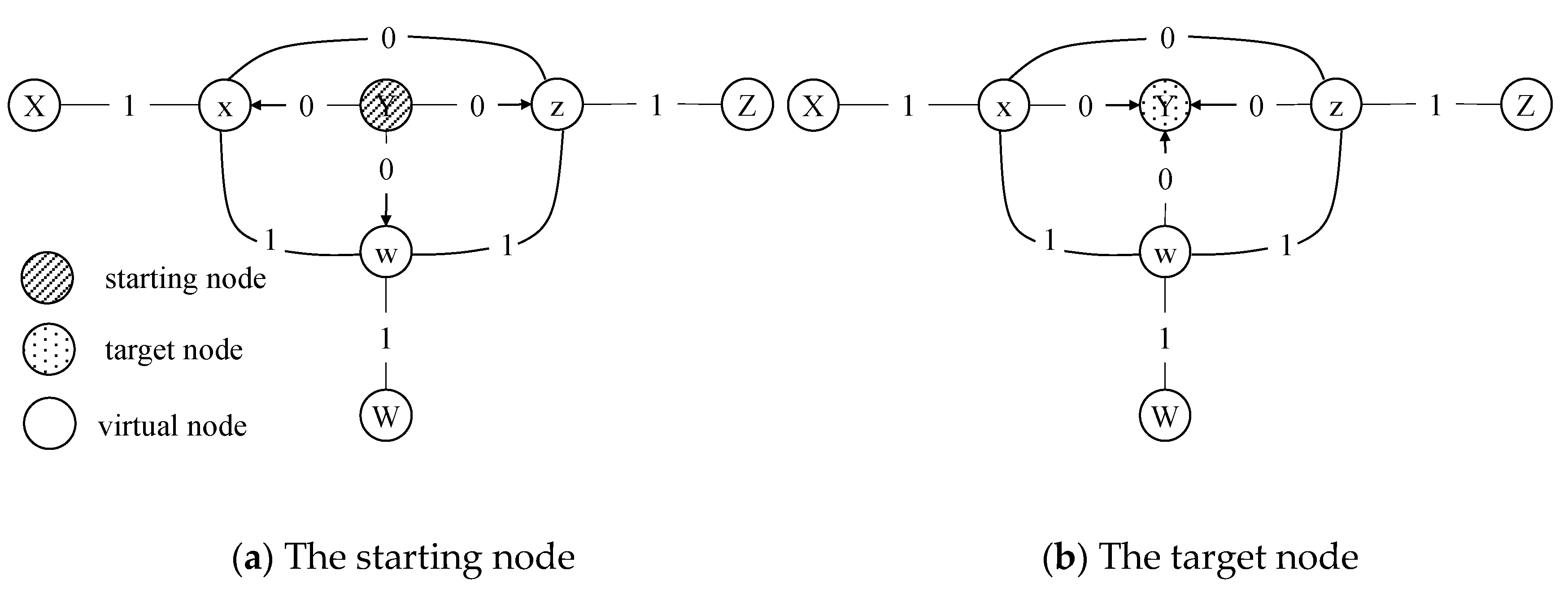
At the same time, considering that node Y can still be used as the starting point and end point, the method shown in
Figure 5 is adopted:
① In order for node Y to be the starting point, introduce three unidirectional edges connecting from Y to the virtual node, and set the weight to zero, as shown in
Figure 5a.
② In order to make node Y as the end point, it is necessary to introduce three unidirectional edges connecting from the virtual node to node Y, as shown in
Figure 5b, and the weight is zero.
③ In order to make node Y both the starting point and the end point, the two kinds of nodes in
Figure 5 are introduced into the new graph, that is, a real node Y is split into two virtual nodes, as shown in
Figure 5. The one shown in 5a is called the starting node, and the one shown in
Figure 5b is called the target node.
At the same time, whether it is the starting node or the target node, when the path needs to pass through the actual node Y, it can only be completed through the virtual path corresponding to Y. This shows that the introduction of these two kinds of nodes does not affect the characteristics of the newly created graph model that can count turns.
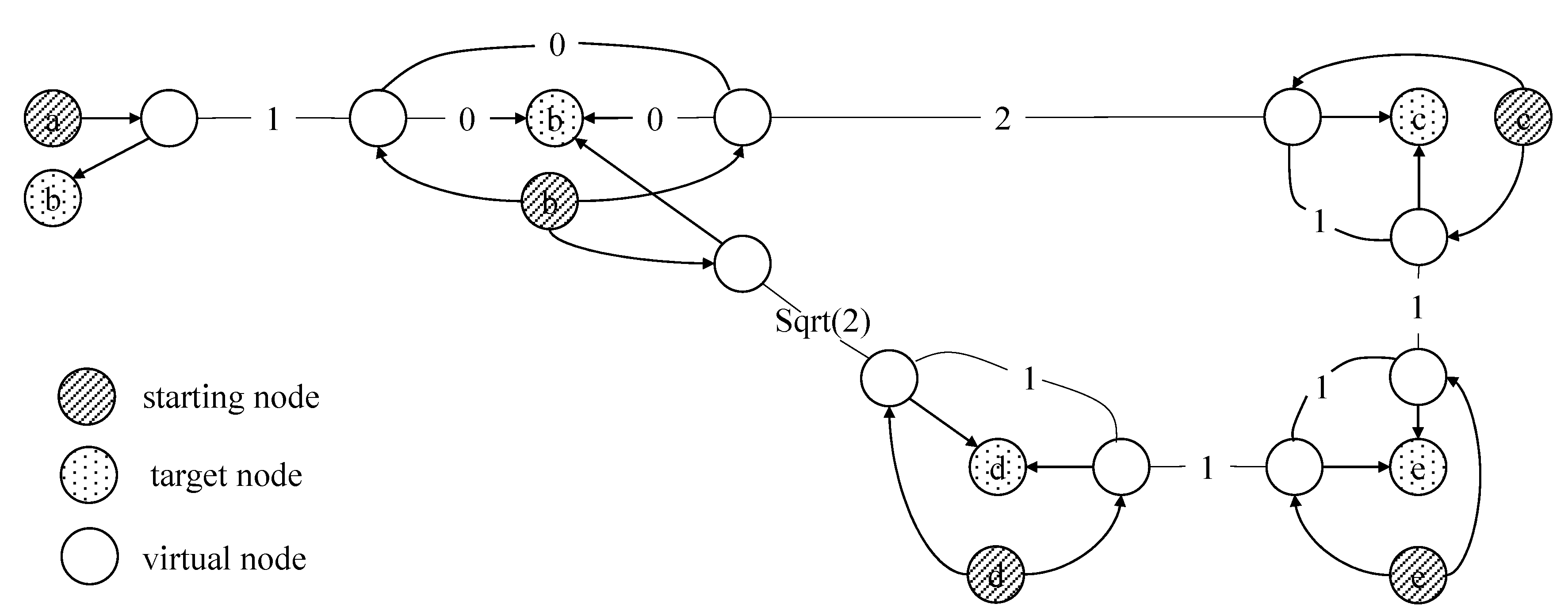
Combining the above two strategies, the original map shown in
Figure 3 can be converted into the map structure shown in
Figure 6. The line segments in the figure all indicate two-way edges, and the arrows indicate one-way edges. The weights of edges without label weights are all 0.
In
Figure 6, taking point b as an example, the actual node b is split into a departure node b and a target node b. The starting node has only the edge connected to the virtual node, and the ending node has only the edge entering from the virtual node. At the same time, there are three white virtual nodes on the three edges connected to b. This method is used to record the turning relationship between the paths.
By performing the conversion according to the above rules, there are two virtual nodes on each edge, corresponding to the two endpoints of an edge. The weight relationship between virtual nodes is the turning relationship between edges. Each actual node is divided into a starting node and a destination node. Finding a path from a to e in the actual problem can be transformed into the shortest path from the starting node of a to the target node of e.
In
Figure 4, the path between any two actual nodes can be transformed into a path from the starting node to the target node and passing through the virtual node. In addition, the path on the new graph has accumulated distance and weight.
For example, to find the optimal path from a to e, at this time, the weight on a→b→d→e is , and the weight on a→b→c→e is 5, so considering the weight of the number of turns , one should choose a→b→c→e as the optimal path. When the weight is not 1, just multiply all the weights on the edges representing the number of turns with to calculate.
2.2.2. Energy Optimal Scheduling Model Based on Hybrid Graph
In the previous section, a simple problem was used as an example to describe the conversion method of simultaneously representing the distance and the number of turns on a same graph. However, the above graphic model can be solved by algorithm only if it is transformed into a mathematical model. In this section, mathematical language is used to describe a general model symbolically, and to discuss how to choose the appropriate algorithm for optimization.
Given a road network , where represents a collection of nodes, and represents a collection of roads:
The weight of the edge is the distance between the nodes, which is represented by the distance matrix . If , it means that there is no edge connection between and .
In addition, different from the general graph, the turning relationship between the edges needs to be considered, denoted as ; if , it means that a turn is needed from to ; if , it means that no turn is needed from to ; in addition, if , then it means that and do not have a common vertex.
In order to simultaneously show the distance between nodes and the turning relationship between roads, a new graph, , is constructed.
Where , represents the set of starting nodes corresponding to the real node ; represents the set of target nodes corresponding to the real node ; and represents the set of virtual nodes on the edge. Obviously, the nodes in correspond to the nodes in one-to-one, and the number is . There will be two virtual nodes on an edge, so there are elements in . Therefore, there are nodes in the graph .
For the set of edges ; where represents the set of edges connected to the departure node in ; represents the set of edges connected to the departure node in ; and represents the set of edges between virtual nodes .
In order to calculate the optimal path on the graph , the weight of the graph is represented by a matrix , which is a matrix. In order to represent the matrix, each node in needs to be numbered according to certain rules.
The nodes in
in this section are numbered from 1 to
in the order of
, while the nodes in
are numbered from
to
rows, that is:
The nodes in
in this section are numbered in the order of the boundary in
, let
, where
, then:
where
represents the virtual node of
; on edge
.
represents the virtual node of
on edge
.
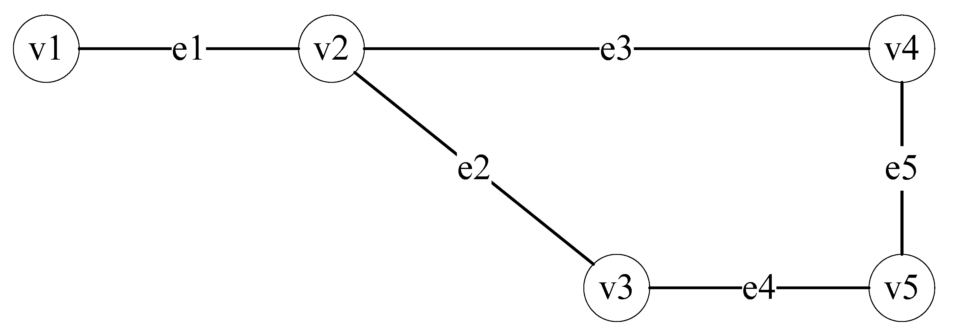
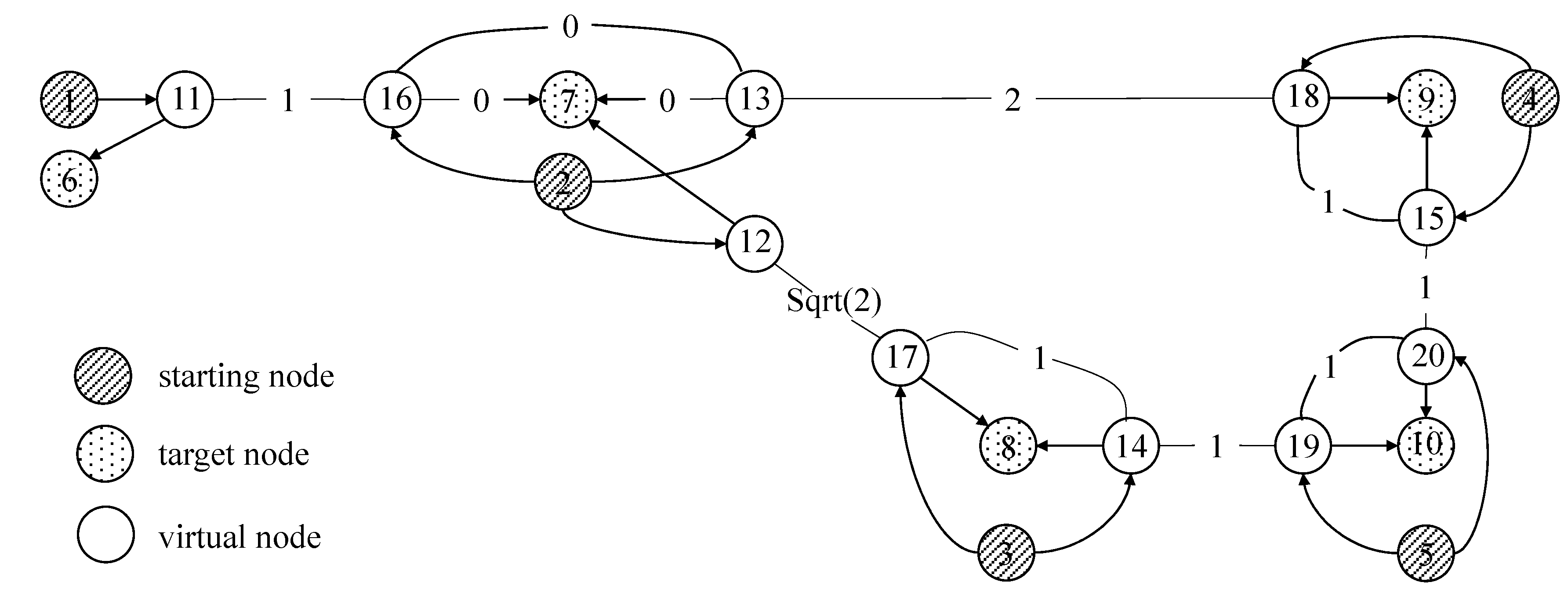
If graph
numbers the nodes and edges according to the situation in
Figure 7, then the number of nodes in graph
is shown in
Figure 8. In
Figure 8, the number of the starting node is from 1 to 5, and the number of the target node is from 6 to 10. The number of the virtual nodes connected to the node with the smaller number on the edge is 11–15, and the number of the virtual nodes connected to the node with the larger number is 16–20.
After numbering the nodes in the graph
, we can follow the rules described in
Section 2.2.1 to give the weight matrix
of the graph
satisfying Equation (5):
where,
① The first case represents , that is, the weight from the starting node to the virtual node is 0;
② The second case represents , that is, the weight from the virtual node to the target node is 0;
③ The third case means that the weight between two virtual nodes on the same edge is the distance between the corresponding real nodes ;
④ The fourth case indicates that the weight of virtual nodes of the same node on different edges is the number of turns between edges multiplied by the weight ;
⑤ In all cases except these four cases, there is no edge connection between nodes, so the weight is .
From the analysis in
Section 2.2.1, we can see that to find the optimal path of
in the graph
, just find the optimal path of
in the graph
. The optimal path problem on the graph
is a classic shortest path problem, which can be solved by the algorithm for solving the shortest path problem.
Five common shortest path algorithms are shown in
Table 1. Among them, the BFS and acyclic algorithms have the lowest complexity, but BFS is an algorithm on an unweighted graph, which is obviously not suitable for solving the problem in this section. Acyclic requires the graph to be a directed acyclic graph, that is, starting from a node, it cannot return to the original node through any path. Obviously, because there are two-way paths on the graph in this section, it is not a directed acyclic graph. The shortest path algorithms that meet the conditions are the Bellman–Ford algorithm and the Dijkstra algorithm. Among them, the complexity of the Dijkstra algorithm is low, and the weights on the map of the shipyard transportation problem are all greater than, or equal to, zero, so the Dijkstra algorithm can be used.
In addition, the reasons for not using the Floyd algorithm that can obtain the shortest distance between all nodes are: (1) in the case of missing paths, the graph has a certain degree of dynamics. If the structure of the graph changes, it needs to be recalculated; (2) the Floyd algorithm cannot obtain the specific shortest path while obtaining the shortest distance.
In summary, this section describes how to generate a graph containing distance and number of turns from a road network. At the same time, the Dijkstra algorithm is chosen to solve the optimal path between two nodes to obtain the global optimal solution of the problem.
2.2.3. Algorithm Solution
The Dijkstra algorithm is a classic algorithm to solve the shortest path problem in graph theory. It is based on an abstract network model, in which the road is abstracted as an edge. The weight of the edge is used to represent the parameters of the road. The algorithm determines the path with the least weight from a certain point to all other nodes in the weighted network. The meaning of weight is broad, which can express distance, quantity, cost, etc. Usually, the smallest weight between two points is called the distance between two points, and the corresponding problem is summarized as the shortest path problem expression.
First of all, the Dijkstra algorithm can be described with the following pseudocode:
for do
end
while do
for do
if then
end
end
end
end
where represents the graph object, is the weight matrix, and is the starting node. During initialization, record the shortest distance from the marked node to the source node , and the predecessor node of each node which means that the previous node in the shortest path is marked as . Then, mark the shortest distance of the source node itself, and then establish a minimum queue according to .
When the algorithm starts to iterate, the vertex of the smallest value in the queue is extracted first each step, and all reachable nodes of is updated. If the distance from node to node plus is less than the original minimum distance of node , is updated, and make the precursor node of .
At the end of the algorithm, records the shortest distance from all nodes to the source node , and records the information of the precursor node. If you want to query the shortest path from node to node , you only need to start from and find the previous node according to , and so on until the node is found. Then the shortest path can be outputted reversely.
2.2.4. Optimal Scheduling Model Considering Path Missing
In the actual dispatch process of the shipyard, a certain route in the road network may be temporarily unavailable. Therefore, in this section, an optimal scheduling model considering path missing is established.
In the road network , suppose the transporter is located at the node , and the transportation task is to move the ship block from the node to the node . When the transporter starts the transportation task, suppose there are some roads temporarily missing in the road network, and the set of these missing roads is recorded as .
The transporter needs to first arrive at node from , and then transport ship block from node to . Considering that the energy consumption ratio of turning and going straight is different when the transport is empty and full, it is necessary to solve the and in sections. Suppose the weight of is and the weight of is .
For
, take the weight as
. After constructing the graph
according to the algorithm in
Section 2.2.2, the weight matrix
is processed as follows, and the missing path is marked as:
which means the weight between the two virtual nodes on this edge is marked as positive infinity. Then, the shortest path on
from the starting node
of
to the target node
of
can be calculated using the Dijkstra algorithm.
Similarly, for
, after constructing the graph
according to the algorithm in
Section 2.2.2, the weight matrix
is processed as follows, and the missing path is marked as:
which means the weight between the two virtual nodes on this edge is marked as positive infinity. Then the shortest path on
from the starting node
of
to the target node
of
can be calculated using the Dijkstra algorithm.
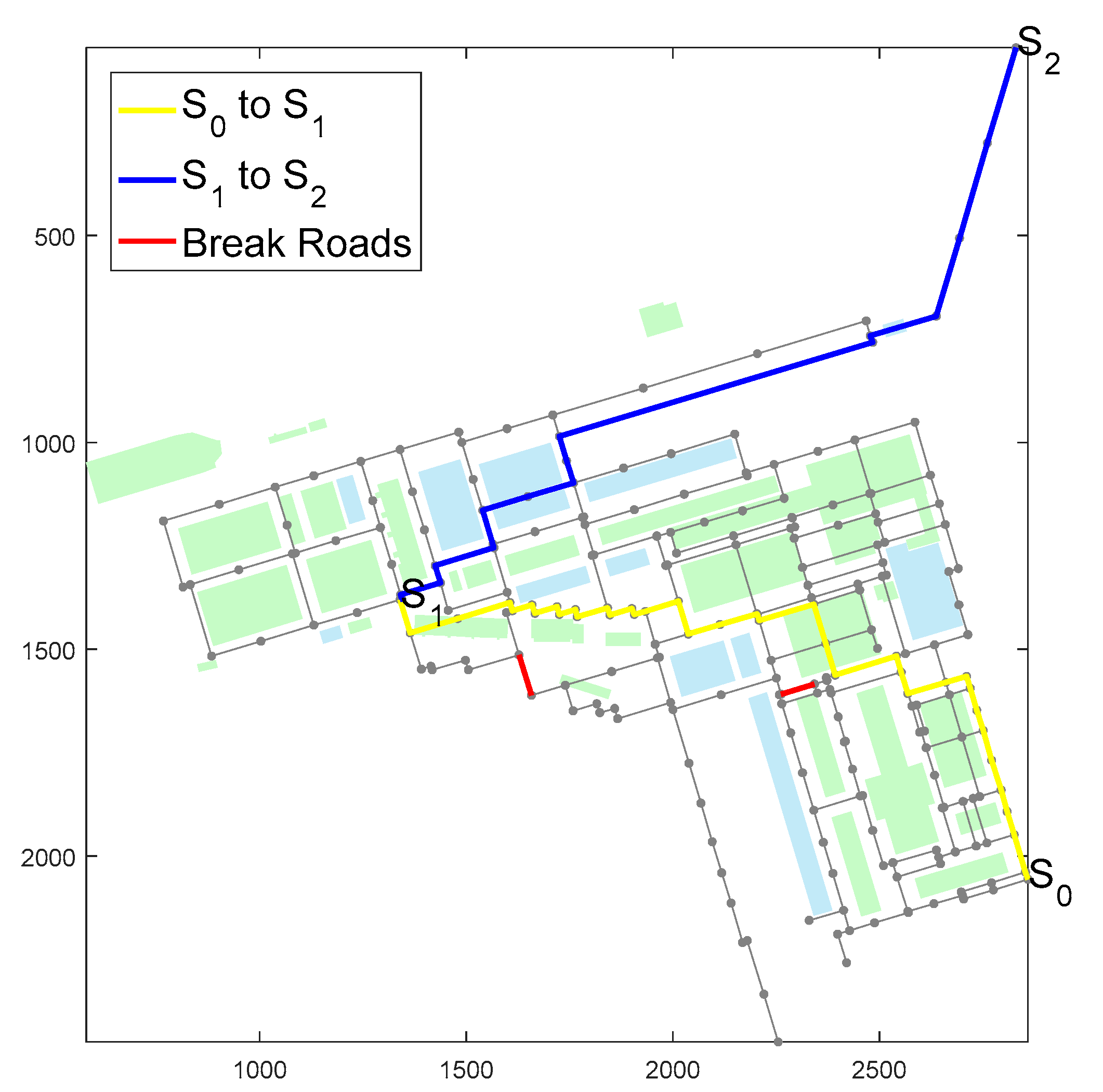
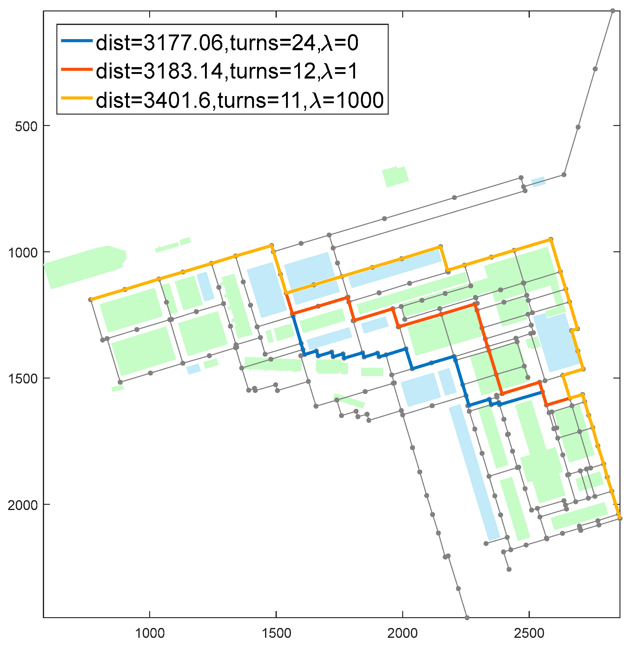
Figure 9 shows a schematic diagram of optimal scheduling. The red road in the picture is the temporarily missing road. The yellow path is the optimal path from the current position of the transporter to the starting point of the mission. At this time, the transporter is empty, and the turning energy is considered negligible, so
; the blue path in the picture is the optimal path from the start of the mission to the end of the mission. At this time, the transporter is loaded, and the turning energy consumption is large. Taking
can get the optimal path in the figure.


