Embedding of a Blade-Element Analytical Model into the SHYFEM Marine Circulation Code to Predict the Performance of Cross-Flow Turbines

Abstract

Our aim was to embed a 2D analytical model of a cross-flow tidal turbine inside the open-source SHYFEM marine circulation code. Other studies on the environmental impact of Tidal Energy Converters use marine circulation codes with simplified approaches: performance coefficients are fixed a priori regardless of the operating conditions and turbine geometrical parameters, and usually, the computational grid is so coarse that the device occupies one or few cells. In this work, a hybrid analytical computational fluid dynamic model based on Blade Element Momentum theory is implemented: since the turbine blades are not present in the grid, the flow is slowed down by means of bottom frictions applied to the seabed corresponding to forces equal and opposite to those that the blades would experience during their rotation. This simplified approach allowed reproducing the turbine behavior for both mechanical power generation and the turbine effect on the surrounding flow field. Moreover, the model was able to predict the interaction between the turbines belonging to a small cluster with hugely shorter calculation time compared to pure Computational Fluid Dynamics.

1. Introduction

The Earth is called “the blue planet”; in fact, water occupies a large part of the Earth’s surface, and moreover, the oceans constitute also immense reserves of energy, which can be exploited only in particular conditions. Close to the coasts, the main resource is represented by tidal currents, which originated from the succession of high and low tides and, for this reason, they are characterized by periodic variations in magnitude and direction that are predictable and quantifiable. The sites of greatest interest in Europe are mainly located in the English Channel [1,2], in the Irish Sea [3], and around Scotland [4], where the proximity to the Atlantic Ocean and the maze of canals, straits, and promontories make the tidal currents particularly intense.

Tidal Energy Converters (TEC) can be classified into seven macro categories, as indicated by the EMEC (European Marine Energy Center) [5]: Horizontal Axis Turbines (HATs); Cross-Flow Turbines (CFTs), also named vertical axis turbines; oscillating hydrofoil, in which a hydrofoil is connected to an oscillating arm; confined turbines in a conduit that concentrates the flow on the device; Archimedes screws that are helical-shaped devices rotated by the water flow; and even tidal kites attached to a turbine that, experimenting lift, allow it to float in the current. Furthermore, there are other types of devices that for the particular design do not fall into the previous categories. Devices are also classified according to the Technology Readiness Level (TRL) [6]; currently, the devices that have reached the greatest maturity are HATs; these are also the most developed devices, as proven by the fact that in 2018, all the seven tidal energy projects founded by the EU for technology at TRL7–9 were conceived for HATs [7].

During the last decade, CFTs intercepted a growing interest thanks to their constructive simplicity and ability to work independently of flow direction. Moreover, by adopting floating platforms, further advantages can be achieved: a generator and gearbox can be set above the sea level, higher currents can be harvested, and the platform motion would just negligibly affect energy output as CFTs still exhibit good performance in skewed flow [8,9]. On the other hand, CFT is affected by low starting torque and lower efficiency compared to HAT. However, experimental and numerical studies proved that CFT gives the best performance when set in counter-rotating closely spaced pairs [10,11,12] in order to exploit advantageous lateral flow acceleration generated by local blockage effects or in farms thanks to a faster wake recovery with respect to HATs [13]. This allows shortening the distance between rows, significantly increasing the power density.

Researchers pay also attention to the environmental impacts [14,15,16,17,18,19] that big farms of marine turbines could potentially cause, such as noise, electromagnetic field production, risk of collision for animals, release of pollutants, and, above all, seabed erosion [20,21] and hydrodynamic impact [22,23]. In fact, since water tends to flow where the hydrodynamic resistance is lower, if the farm occupies almost the whole width of a channel or strait, alterations could occur in the path and speed of currents. Further environmental damages, correlated to hydrodynamics changes, could be the perturbation of the natural transportation of sediments [24,25], chemical nutrients, and phytoplankton [26], which could affect the marine habitat and then the entire food chain. For these reasons, it is crucial to develop assessment tools for investigating the flow perturbations on a large scale as well as the power yield for any farm layout. In this regard, the state of the art of studies based on software of marine circulation shows that the interest of scientists is focused on the assessment of the hydrodynamics effects without considering the turbine geometrical and operating parameters. To clarify better, in all the existing approaches, the turbine power coefficient (or, the related to it, thrust coefficient) is an input of the problem, which is used to calculate the loss of momentum in the flow (i.e., the local impact of the turbine on the environment) by means of the equations of the Actuator Disc (AD) theoretical model [27]. This simplification came from the need to adopt not extremely fine grids in the turbine farm region in order to limit calculation times. In fact, although grid local refinements were done with respect to the far field grid, the grid was still so coarse that a single cell contained the entire turbine or even (in early studies) more than one turbine. Now, just a few investigations can be found, all concerning HATs, in which spatial resolutions no greater of 1/10th of the turbine diameter are set for the turbine and the wake regions [28,29]. However, even in these recent approaches, the turbine performance is assumed to be known, since they only make use of the AD theory. Meanwhile, in case of CFTs, neither the AD nor the turbine analytical models have ever been incorporated into a marine circulation code.

In the present study, a simple Blade Element model of CFT is embedded into the open-source SHYFEM ([30,31,32], and reference therein) marine circulation code, according to the Blade Element Momentum (BEM) theory [27]. The novelty respect to the current approaches is that the turbine geometrical parameters and the rotation speed are included, since they determine the loading (lift and drag) on the blade. It must be noted that hybrid BEM-CFD models for CFTs are increasingly used by engineers to predict the turbine performance in applications of practical interest [33,34,35,36,37,38]. However, despite the computational costs being significantly less than in the case of high-fidelity fully CFD simulations, the complexity of the models and the refinement of grids limit their use to the simulation of a single turbine. This work is a first step toward the implementation of a hybrid BEM-CFD tool of marine circulation to implement not only to predict the large-scale impact of tidal energy extraction but also to optimize the turbine geometry and the farm layout in real environments. For simplicity, the study is 2D, and the easiest method to subtract momentum from the flow field—that is, the bottom friction—is adopted. Our objective is to answer these questions: “Is it possible to describe the blade torque evolution during a revolution with grid local refinements that are comparable to the finest ones nowadays adopted in AD marine applications? Is our approach adequate to capture all the turbine main effects on the surrounding flow field, therefore not only the wake characteristics but also the interactions between closely spaced turbines that are responsible for a power increasing in CFTs?”

2. Methodology

This chapter describes the methodology underlying the work, starting with the validation of the pure CFD model, which is then used to validate the hybrid models instead of experimental data. Subsequently, the foundations of the hybrid BEM-CFD approach are recalled, and then, the grid sensitivity analysis is done with the hybrid model implemented for the software ANSYS-Fluent [39]: this is useful in order to individuate a grid local refinement suitable for marine codes. Finally, the BEM-SHYFEM formulation is presented with a focus on the bottom friction treatment.

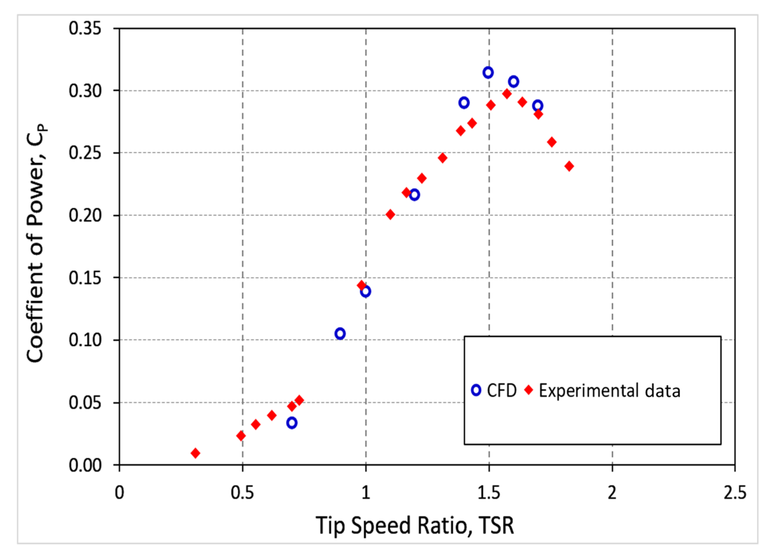
2.1. Preliminary Validation of the ANSYS CFD Model

The results achieved with the hybrid BEM-CFD models (based on ANSYS or SHYFEM) will be compared with pure CFD simulations in the next sections, since no experimental data are available for the hydrokinetic turbine of interest. Of course, this method requires a preliminary validation of the pure ANSYS-Fluent model with respect to other experimental data from the literature in order to verify the reliability of the setting choices summarized in

Table 1. ANSYS’s setups for both pure Computational Fluid Dynamics (CFD) and hybrid ANSYS model.

Turbulence Model	SST k-ω
Solution Methods	Pressure–Velocity Coupling	Scheme SIMPLEC
Spatial Discretization	Gradient	Least Squares Cell-Based
	Pressure	2nd Order
	Momentum	2nd-Order Upwind
	TKE	2nd-Order Upwind
	Specific Dissipation Rate	2nd-Order Upwind
	Transient Formulation	2nd-Order Implicit
Transient Formulation	Second-Order Implicit
Residuals	0.0001

and adopted for both the ANSYS approaches: full CFD and hybrid.

The preliminary validation task was done with respect to the data achieved by Bravo et al. [40] in a wind tunnel for a CFT equipped with 3 straight blades, in which the airfoil is the symmetrical NACA0015. These experimental data were chosen due to the relatively high Reynolds (with respect to typical wind tunnel and water flume tests) and low blockage ratio (thanks to the very large section of the wind tunnel). The turbine’s performance is usually given by the Power Coefficient, C_P, which is defined as:

$$C_P=\frac{P}{\frac{1}{2}\rho U^{3}A}$$

(1)

where P is power generated, ρ is the density, U is the free stream flow velocity, and A is the cross-sectional area of the rotor that, in case of CFTs in 2D domains, corresponds to the turbine diameter, d. The curve C_P-TSR describes the turbine performance as a function of the Tip Speed Ratio, TSR, which is defined as:

$$TSR=\frac{R\Omega }{U}$$

(2)

where R is the turbine radius and Ω is the rotational speed. It is well known that C_P predicted from 2D simulations is overestimated since important 3D effects—first of all, the blade tip losses—cannot be taken into account. In particular, due to the moderate value of the chord-based aspect ratio of this turbine (blade length/chord = 7.5), significant tip losses are expected. Since these 2D CFD simulations cannot directly predict tip losses, a correction factor must be used to reduce C_P afterwards in order to allow a meaningful comparison with experimental data. On the basis of the study [41], a plausible value of tip losses for a CFT with this aspect ratio could be ≈25%. Figure 1 depicts the results of CFD (having already subtracted 25% from the 2D original predictions) compared to the experimental results obtained for a flow speed of 10 m/s [40]. It can be seen that the trend, the optimal TSR, and the maximum C_P are well matched, with just a small discrepancy in the optimal TSR. In order to match the experimental data at the low TSRs, particular attention was paid to the quality of the calculation grid (Figure 2); in fact, around each airfoil, many layers of regular quadrilateral cells were created of increasing height with exponential law starting from the blade wall. The following parameters have been kept for all the 2D grids with blades adopted in this study: 710 cells around the blade profile; c × 4 × 10⁻⁶ (where c is the airfoil chord) for the height of the first layer of cells at the blade wall; 1.06 for the cell height growing ratio; 110 layers around the blade profile. It should be observed that the cell smallest height depends on the particular chord value. In this way, around each blade, a very fine and high-quality grid is obtained for a distance of about 1.5 × c from the airfoil/hydrofoil.

It could be objected that the experiments adopted in the present work to validate the pure CFD model refer to a turbine [40] with a moderately lower Reynolds and a significantly greater solidity than that of interest. However, we are confident that since the pure CFD model provides realistic results even under more critical conditions for flow separation phenomena (as characterized by a lower Reynolds and higher solidity) than the conditions to which the hybrid models are applied in the present study, it can be considered reliable.

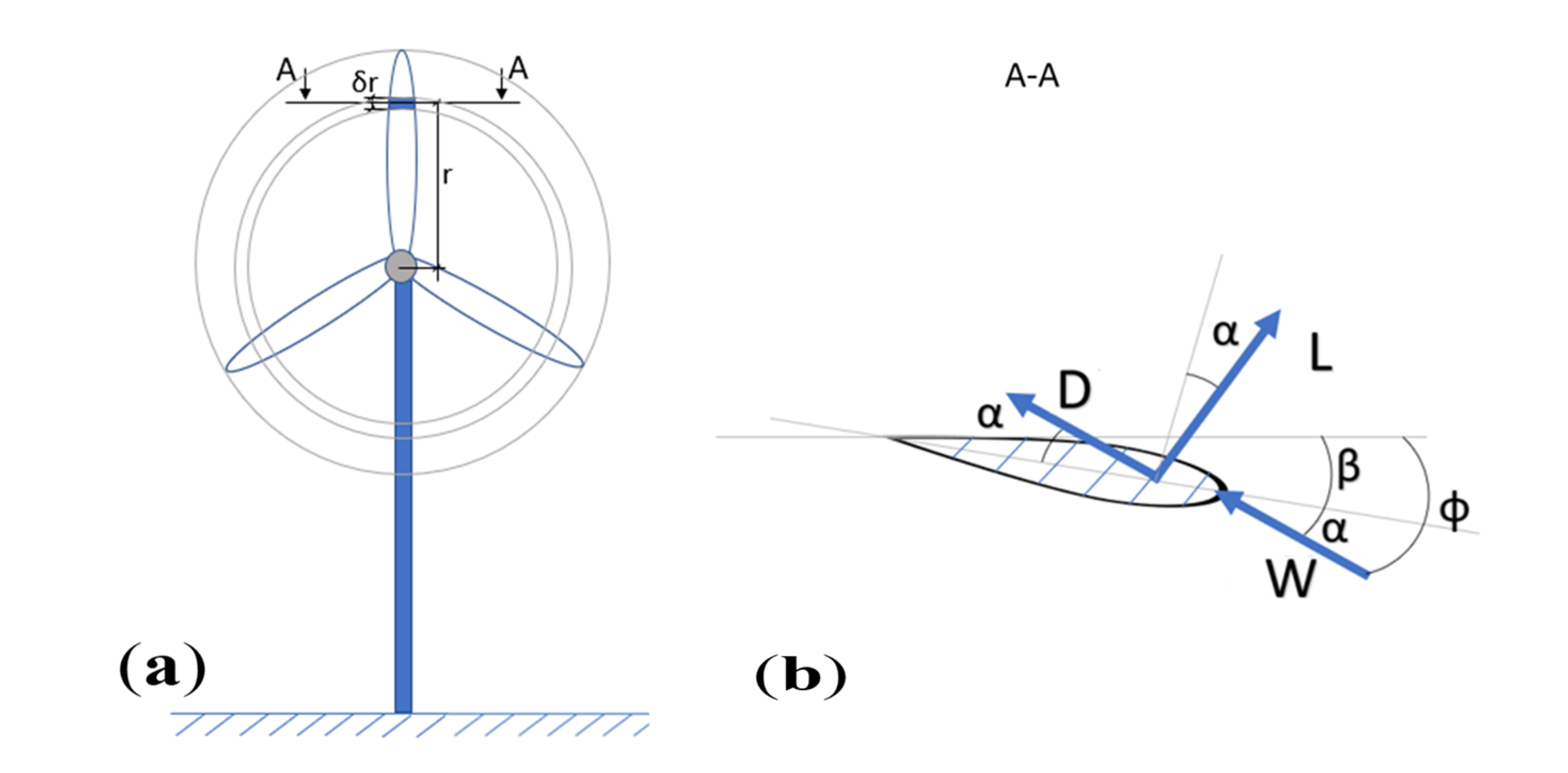
2.2. BEM Theory Basics

The hybrid model (regardless of whether it is ANSYS-Fluent or SHYFEM) is based on the BEM theory. According to this theory, the “blade element” is defined as the blade section placed at a generic radius r of infinitesimal thickness δr; the forces acting on the B blade elements (where B is the total blades number) are responsible for the axial momentum loss to which the flow passing through the ring of infinitesimal thickness is subjected. As shown in Figure 3, the resulting force can be split in lift and drag, which are directed normal and parallel to the relative velocity W (vector sum of the flow absolute velocity and the blade velocity) approaching the blade element. Important angles that have to be defined are the attack angle α, the pitch angle β, and the inflow angle Φ, which is a sum of α and β. It should be noted that Φ is the angle between the incoming flow and the rotor plane.

The values of lift δL and drag δD acting on the blade element are calculated as follows:

$$\delta L=\frac{1}{2}\rho W^2{C}_{L}c\delta r\hspace{1em}\hspace{1em}\hspace{1em}\delta D=\frac{1}{2}\rho W^2{C}_{D}c\delta r$$

(3)

where C_L and C_D are the lift and drag coefficients of the particular hydrofoil that is considered. C_L and C_D depend on the attack angle and Reynolds number, and they need to be measured experimentally in a wind tunnel. Then, the expressions of torque $\delta Q$ and power $\delta P$ are

$$\delta Q=\left(\delta Lcos\left(\Phi \right)+\delta Dsen\left(\Phi \right)\right)r\hspace{1em}\hspace{1em}\hspace{1em}\delta P=\delta Q\times {\Omega }_{.}$$

(4)

By applying the principle of action and reaction, equal and opposite forces are impressed on the flow: in fact, in hybrid models, the physical blades are not simulated, and therefore, they are not included in the computational domain. The domain region that is swept by the blades is instead represented by fluid cells where momentum source terms are applied to slow down the flow. The source terms are in the form of forces per unit of volume:

$$S_{i,j}=\frac{F_{i,j}}{r\Delta \theta \Delta h\Delta r}$$

(5)

where $F_{i,j}$ is the force applied on the j-th cell of the grid in the i-th direction, $\Delta \theta$, $\Delta h$, and $\Delta r$ are the azimuthal, height, and radial extension respectively of the considered blade element.

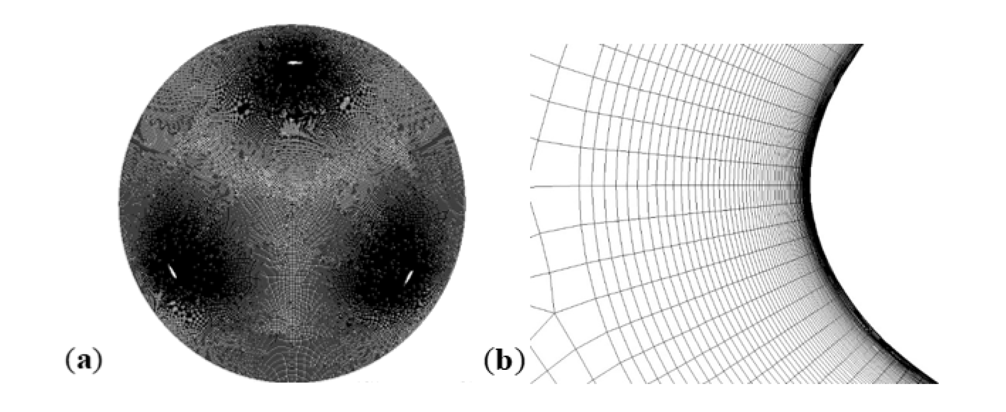
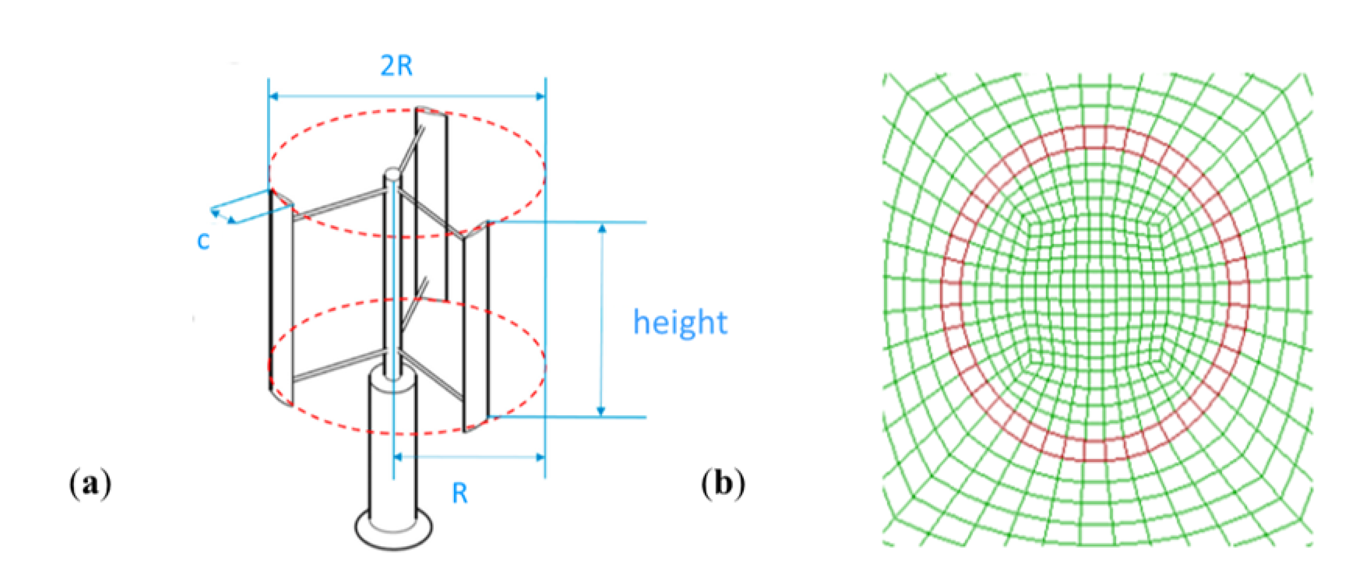
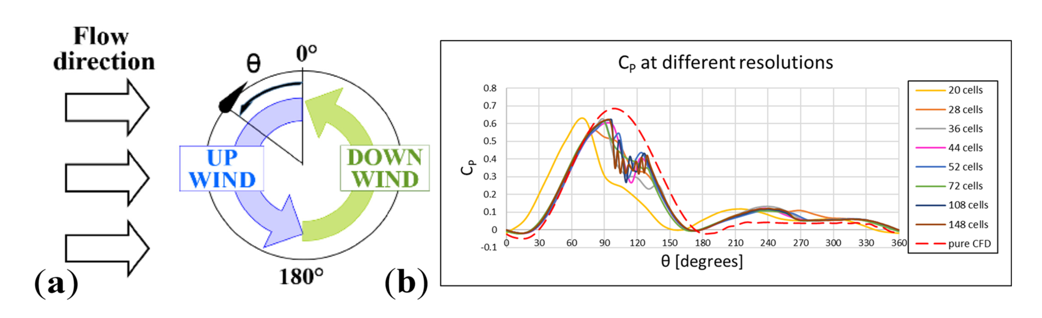
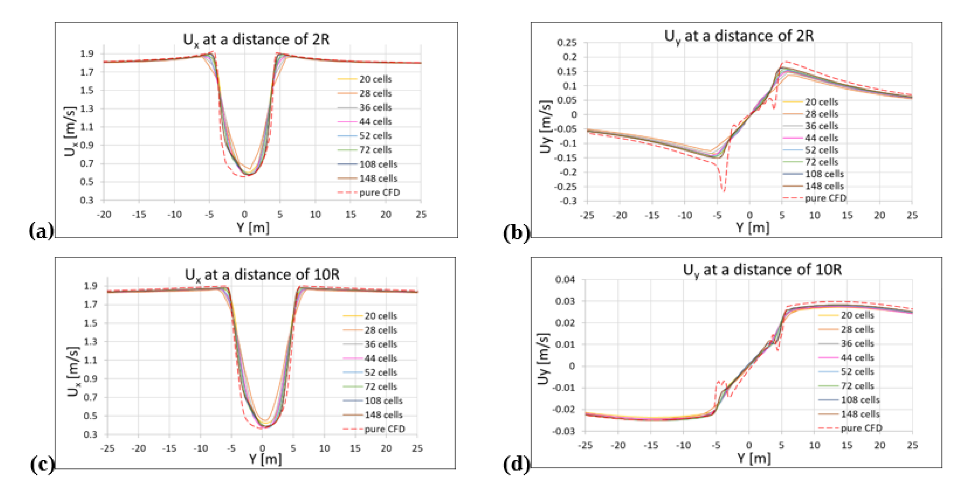
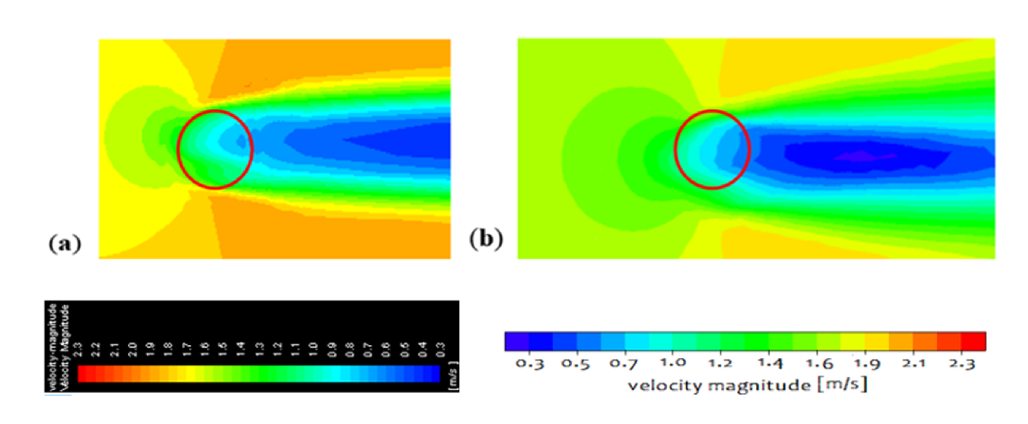
2.3. Grid Effect Analysis With the ANSYS Hybrid Model

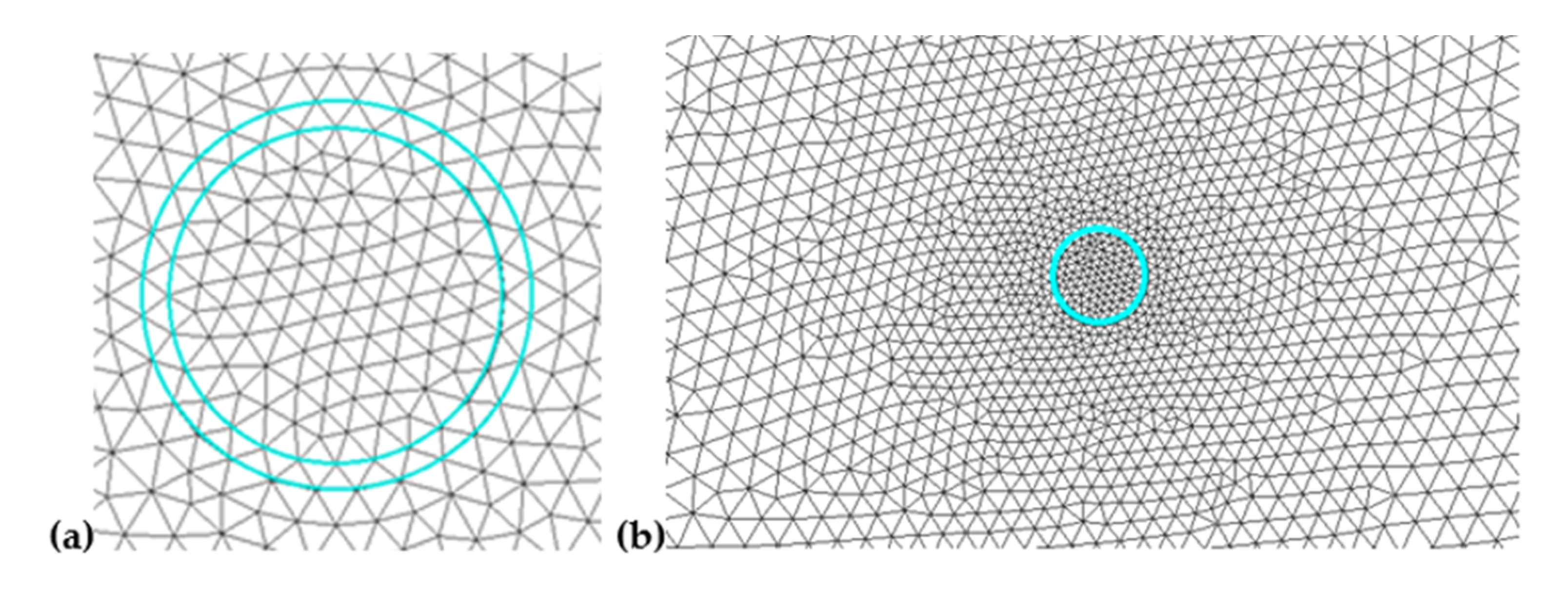
The BEM model was implemented by Rocchio et al. [35] in the ANSYS-Fluent general purpose CFD code. In the present work, for all the sub-models, we kept the same coefficients that were tuned in the original work [35], despite the tidal turbine subject of this study having a higher solidity with respect to the original wind turbine. The reason for this choice was to verify the robustness of the model to differences in turbine geometry. In this section, we characterize the BEM-ANSYS hybrid model behavior in terms of predicting the performance of a tidal CFT and the wake generated by it, and we compare it with pure CFD simulations, varying the grid refinement. The aim was to check if a grid refinement compatible with marine circulation codes, and then relatively low resolution, is still enough to describe the details of the blade torque evolution during the turbine rotation and the wake main characteristics.

The ANSYS hybrid model is implemented in the software by means of a User-Defined Function (UDF). The hydrokinetic turbine here considered is the Kobold turbine with three straight blades [42] (Figure 4a): the height is 6 m, the radius is 3 m, and the chord is 0.4 m. The solidity σ is 6.37%, and it is defined as

$$\sigma =\frac{Bc}{2\pi R}$$

(6)

The hybrid grid shows the ring (in red in Figure 4b) of fluid cells where source terms are applied. It can be seen that the kind of grid is “structured multi-blocks” that are only made of quadrilateral cells. The domain dimensions are 64R and 50R, respectively in the x and y direction. The time step is set by dividing the revolution period for the number of ring’s cells or for 720, respectively for the hybrid model and pure CFD. In both cases, 60 turbine revolutions have been simulated. The flow inlet velocity is fixed at 1.75 m/s; other setups are the same as already listed in Table 1.

The UDF [35] has several sub-models that are used to simulate phenomena such as dynamic stall, tip losses, and virtual cambering, yet in this work, only the dynamic stall sub-model [43] has been considered for simplicity. A sensitivity analysis to the grid refinement was carried out by increasing progressively the number of cells on the ring from 20 to 148. Figure 5a depicts the definitions commonly adopted to describe the blade path of a CFT during a rotation: the upwind path occurs for θ going from 0° to 180°; the downwind path occurs for θ going from 180° to 360°. Figure 5b shows the evolution of the instantaneous C_P of the single blade during one revolution; the hybrid model is sufficiently able to capture the main detail of the C_P evolution at the different grid resolutions except for the coarsest case (i.e., 20 cells on the ring). The anomalous and unphysical drop in the upwind curve (θ ≈ 95°–110°) is due to the virtual camber sub-model. In fact, this sub-model is greatly sensitive to the turbine solidity: for solidity lower than 4–5% it is stable, but it does not adequately work for the solidity of the Kobold turbine, therefore leading to the choice to switch off this sub-model.

It is worth noting that since our present hybrid model implementation is just 2D, at present, is not possible to reproduce the fast wake recovery that can be experimentally observed, and that is mainly due to the vertical advection induced by the evolution of the tip vortices [44]. Therefore, also for the wake characteristics, we preferred to compare/validate the hybrid models against results from pure 2D CFD, since it undergoes the same limitation. Wake velocity profiles of the velocity x and y components are matched for all the resolutions (Figure 6), with the exception of the coarsest ones (20 and 28 cells on the ring). Based on these preliminary outcomes, the ring was divided into 44 cells in order to have a not too-fine local resolution, and it would be compatible with marine circulation codes. In dimensionless terms, this refinement corresponds to a cell size of 1/7R.

Figure 7 shows the behavior of the blade instantaneous C_P calculated, in case of 44 cells on the ring, with the hybrid model and with pure CFD for several values of the turbine TSR.

The qualitative trend is similar for the hybrid and the CFD cases at different TSR values while quantitative discrepancies are noticeable; these differences are due to the fact that the ANSYS hybrid model was validated versus experimental data concerning low solidity wind turbines, as reported in [35]. Yet, it should be noted that the qualitative behavior is captured anyway. For a better quantitative matching of the turbine behavior, it will be necessary to tune some of the sub-model’s coefficients versus experimental data available for higher solidity CFTs. However, in this work, we are not interested in improving the hybrid model developed in [35] for a water system: we will assume the model to be acceptable in order to capture the qualitative behavior of a hydrokinetic device, and the ANSYS hybrid model results will be adopted to make a comparison with the SHYFEM hybrid model. What is expected is to record the same behavior for the turbine in both models, because the analytical model underlying the SHYFEM hybrid model is the same as that of the ANSYS hybrid model.

It must be specified that for the hybrid simulations represented in Figure 7, the virtual camber model was disabled: in purely analytical and in hybrid BEM-CFD tools, this model is useful to reproduce the curvature of the flow on the hydrofoil during its rotational motion [45]. In a pure CFD simulation, this effect is naturally reproduced, while in a hybrid model, without a physical blade, this effect is taken into account by giving a virtual camber to the hydrofoil. By doing this, the symmetrical hydrofoil in CFD corresponds to the cambered hydrofoil in hybrid model, as shown in Figure 8a, where a is the axial induction factor. A curved hydrofoil in CFD corresponds to a symmetrical hydrofoil in hybrid simulations, as shown in Figure 8b. In order to keep the virtual camber sub-model in our hybrid simulation switched off, it was necessary to adopt for the pure CFD a hydrofoil with an opposite curvature in order to compensate, and then to cancel, the flow curvature.

2.4. SHYFEM Grid

To reproduce the same resolution in the turbine zone, the SHYFEM finite-elements grid has a ring with 56 triangular elements (Figure 9) with an average size corresponding to a little more than 1/9R.

The dimensions of the computing domain are the same as those used for the ANSYS grid, and in this case, the resolution is not uniform all over the grid: an unstructured mesh easily allows high refinement in the area of interest and progressively lowers the resolution, up to 4/3R at the domain boundary. At 2R downstream from the turbine axis, the element’s averaged size is about 1/3R, while at 8R, it is about 2/3R.

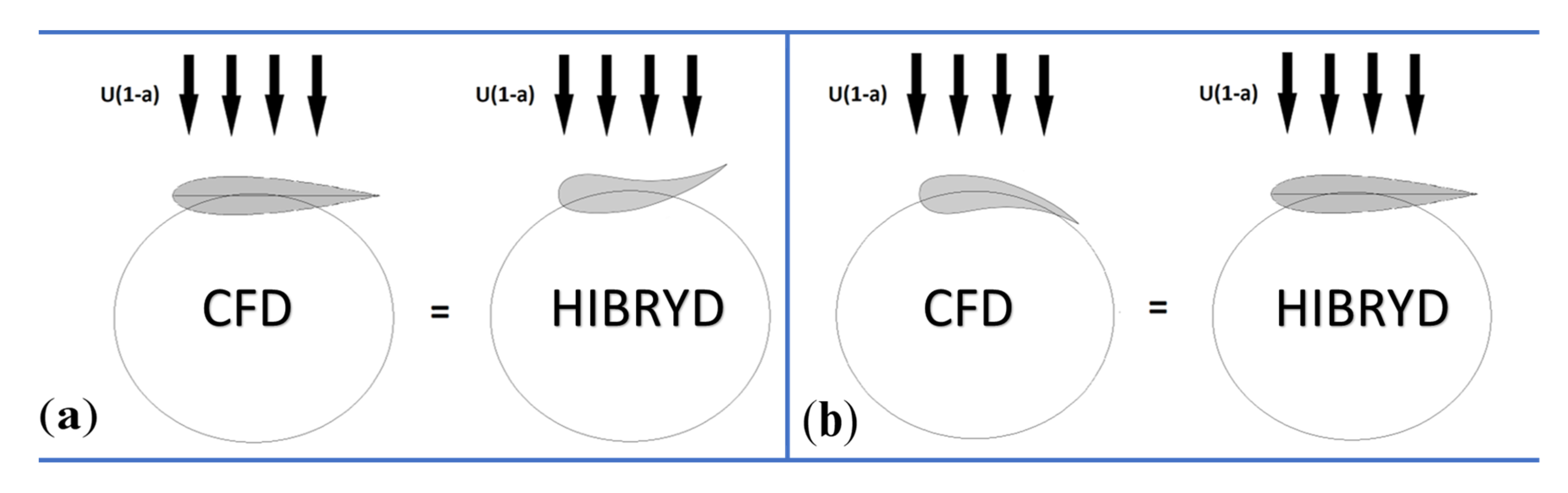
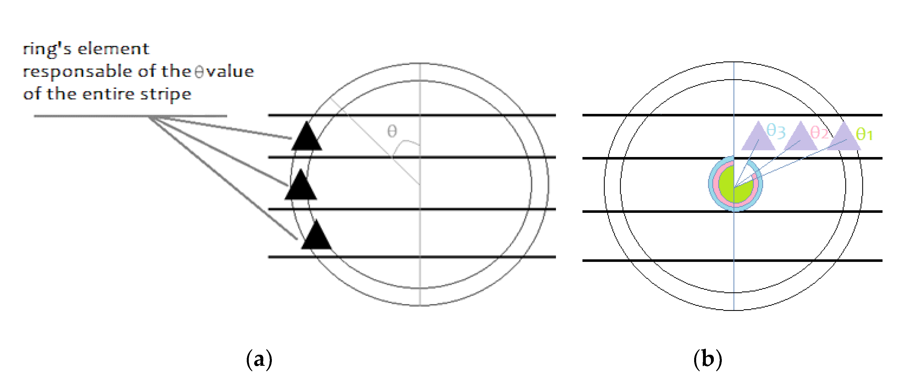
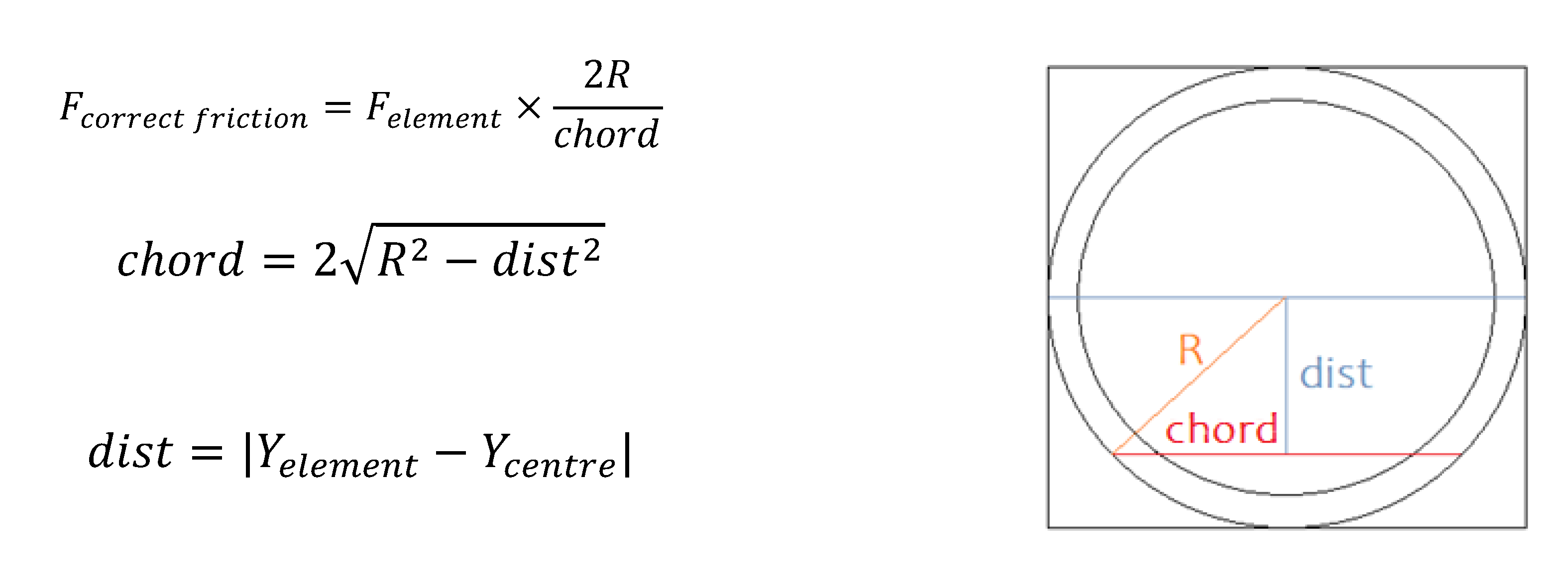
2.5. Friction’s Formulation in the SHYFEM Hybrid Model

Differently from ANSYS Fluent, SHYFEM simulates the effect of the turbine’s presence not as a momentum source but as a variation on bottom friction. In the present formulation, the model solves the shallow water equations, reproducing the barotropic transport and reflecting the horizontal flow patterns around the turbines:

$$\frac{\delta U}{\delta t}+gH\frac{\delta \zeta }{\delta x}+FU+X=0$$

(7)

$$\frac{\delta V}{\delta t}+gH\frac{\delta \zeta }{\delta y}+FV+Y=0$$

(8)

$$\frac{\delta \zeta }{\delta t}+\frac{\delta U}{\delta x}+\frac{\delta V}{\delta y}=0$$

(9)

where H is the height of the water column given by the sum of ζ, the level of the free surface of the water, which is variable due to, e.g., waves and tides, and h, the undisturbed water column depth; F is a coefficient that describes the time scale of friction; g is the gravitational acceleration; and X and Y are explicit terms forcing the hydrodynamics, such as wind and atmospheric pressure. Finally, U and V are transports.

$$U=\underset{-h}{\overset{\zeta }{{\displaystyle \int }}}udz\hspace{1em}\hspace{1em}\hspace{1em}V=\underset{-h}{\overset{\zeta }{{\displaystyle \int }}}vdz$$

(10)

The shallow water approximation assumes that the horizontal scale of the process is larger than the vertical scale, and the water column is reproduced by a unique layer. SHYFEM, in its 3D formulation, assumes the Shallow Water approximation in order to solve the flow field in each layer: then, vertical advection and viscosity terms induce the vertical dynamics, allowing connection among layers on the water column; this means that an exchange of mass, temperature, and other variables occur between different layers. In the present implementation, as a first substantial simplification, the focus is on the reproduction of the horizontal current field around the turbine; therefore, a 2D approach is preferred, and the effects of the turbine’s presence in water in terms of slowdown on barotropic flows are induced by variation in bottom friction. Since this is the first application of a hybrid model with a BEM approach in a marine circulation model, it was decided to adopt the friction method to allow a more stable calculation. This kind of approach is suitable for 2D application, while it would not be suitable for a 3D simulation. In coastal and transitional environment studies, the different friction formulations are used to reproduce different bottom environments (e.g., rocky, muddy, sandy) and concur in allowing correct sediment transport dynamic, deposition–resuspension, or wave pattern reproduction [46,47]. The friction is introduced in the Shallow Water equation thanks to the F term defined as follows:

$$F=\lambda \times \frac{\left|UV\right|}{H^2}$$

(11)

where

$$\left|UV\right|=\sqrt{U^2+V^2}.$$

(12)

$\lambda$ represent the drag coefficient (a-dimensional) that can be set constant. The formulation of $\lambda$ in the grid area where the turbine is located, according to other works found in the literature [1,48], is given by:

$$\lambda =\frac{n_B}{icount}\times \frac{h\sqrt{L^2+D^2}}{\rho \times \frac{\left|UV\right|}{h^2}\times U}$$

(13)

where $\lambda$ is proportional to the force module that the blade would have experimented. Lift and Drag (L and D) forces are given for a single blade and are expressed per unit area of the grid element to which they are applied. Forces are applied to a ring’s cell as if a single blade is present in that cell for the entire revolution period. Since this is similar to having the blade omnipresent in the whole ring at any time, it is necessary to divide the forces for the time frame in which the blade is effectively present in the cell, dividing the forces for the number of the ring cells icount: the effect is to have a blade that rests on every element just for an icount-th of the revolution time. Furthermore, since there are B blades, it is necessary to multiply forces for the number of blade $n_B$. Developing the equation, we obtain:

$$\lambda =\frac{n_B}{icount}\times \frac{h\sqrt{{\left(\frac{1}{2}\left(\frac{\rho c{W}^2}{are{a}_{ele}}\right)\left(C_L+C_D\right)\right)}^2}}{\rho \times \frac{\left|UV\right|}{h^2}\times \left|UV\right|}$$

(14)

$$\lambda =\frac{n_B}{icount}\times \frac{\frac{1}{2}hc{W}^2\sqrt{{\left(C_L+C_D\right)}^2}}{are{a}_{ele}\times \frac{\left|UV\right|}{h^2}\times \left|UV\right|}$$

(15)

Applying friction only on the ring’s elements, we can see fluctuations in the downwind performance curve, as shown in Figure 10. This simulation has been made at the optimal Tip Speed Ratio of 2.7.

The dynamic stall model in downwind leads to unrealistic downwind fluctuations; therefore, it was decided to disable it. This approximation is acceptable, because the downwind flux is slowed down by the power generation occurred in upwind: it is unlikely of a having high angle of attack that can cause downwind stall.

On the other hand, applying the friction only on the ring’s elements (with the dynamic stall model disabled in downwind), the performances are not similar to those obtained by pure CFD simulations: the upwind production is reduced, and the downwind production is excessive (Figure 10).

Therefore, a different approach was needed to improve the hybrid model results: the turbine-dependent friction has been applied not only on the ring’s elements but also on the inside elements. For the inside elements, the θ value is given in a different way: for the upwind elements, we divide the turbine in 18 virtual stripes and assign the θ value for all the inside elements as the one of the ring’s element on the same stripe (Figure 11a); for the inside downwind elements, the θ value is assigned as the geometrical angle of the element (Figure 11b).

Applying the friction on the entire disc, the flow that passes through the central stripe of the turbine is excessively slowed down, since there are many elements with turbine-dependent friction. On the contrary, the flow that passes through lateral stripes of the turbine is not slowed down enough. Making the turbine virtually square prevents these inconveniences, multiplying the number of turbine elements by a 1.2732 factor that represents the ratio between the surface of a square with edge 2R and a disc with radius R, and then adopting a 2R/chord factor to correct the friction in each element (see Figure 12). The chord is the geometrical chord of the circle.

This method allows having an appropriate imposition of turbine-dependent friction to a wider surface without having problems, such as premature slowdown of the flow, to reproduce the blade’s power production along a revolution.

3. Results of the BEM–SHYFEM Hybrid Model

The chapter shows the predictive capability of the SHYFEM hybrid model for a single turbine in comparison to a pure CFD and ANSYS hybrid model and for two clusters of three turbines in comparison to pure CFD. Some considerations about grid resolution effects are presented.

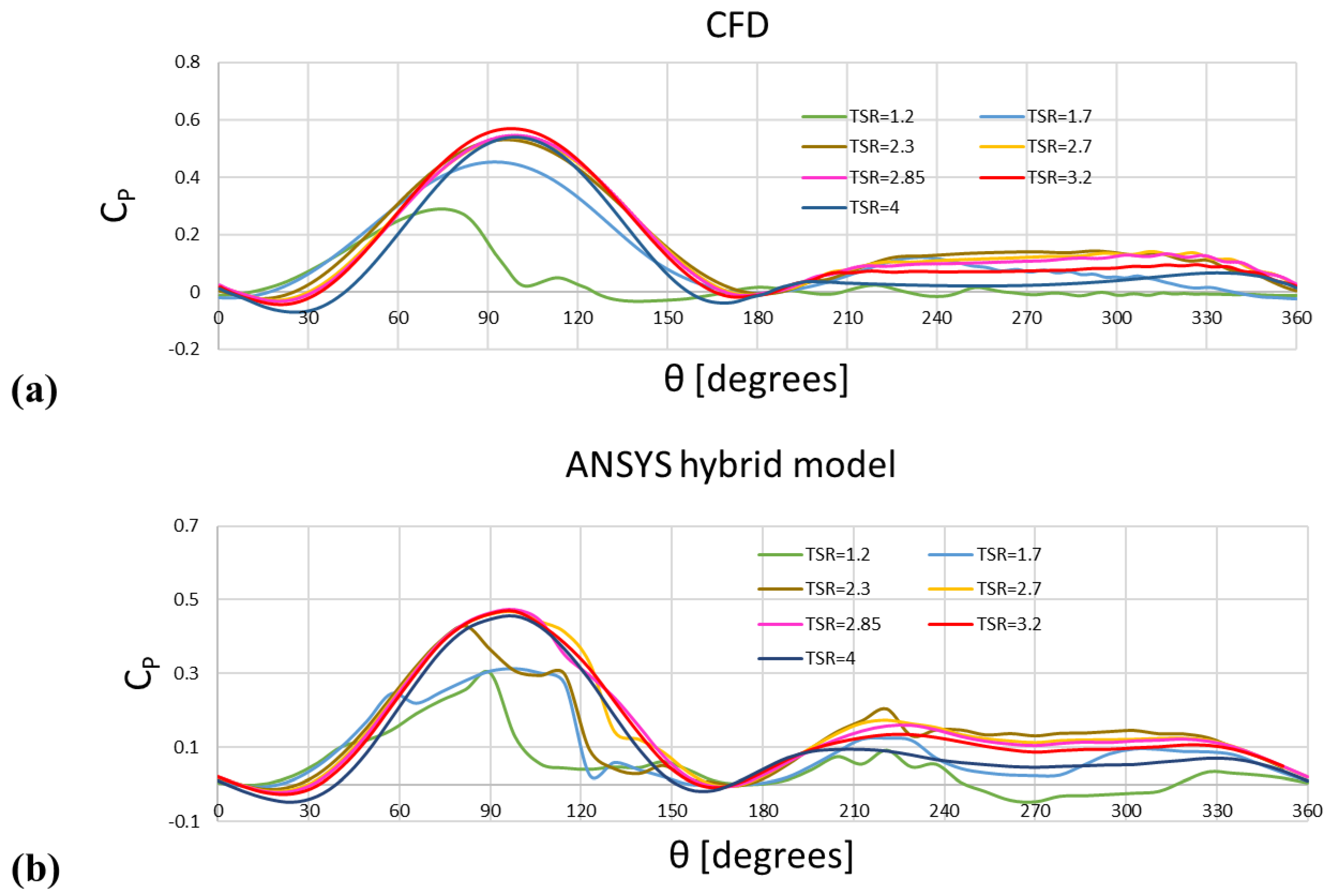
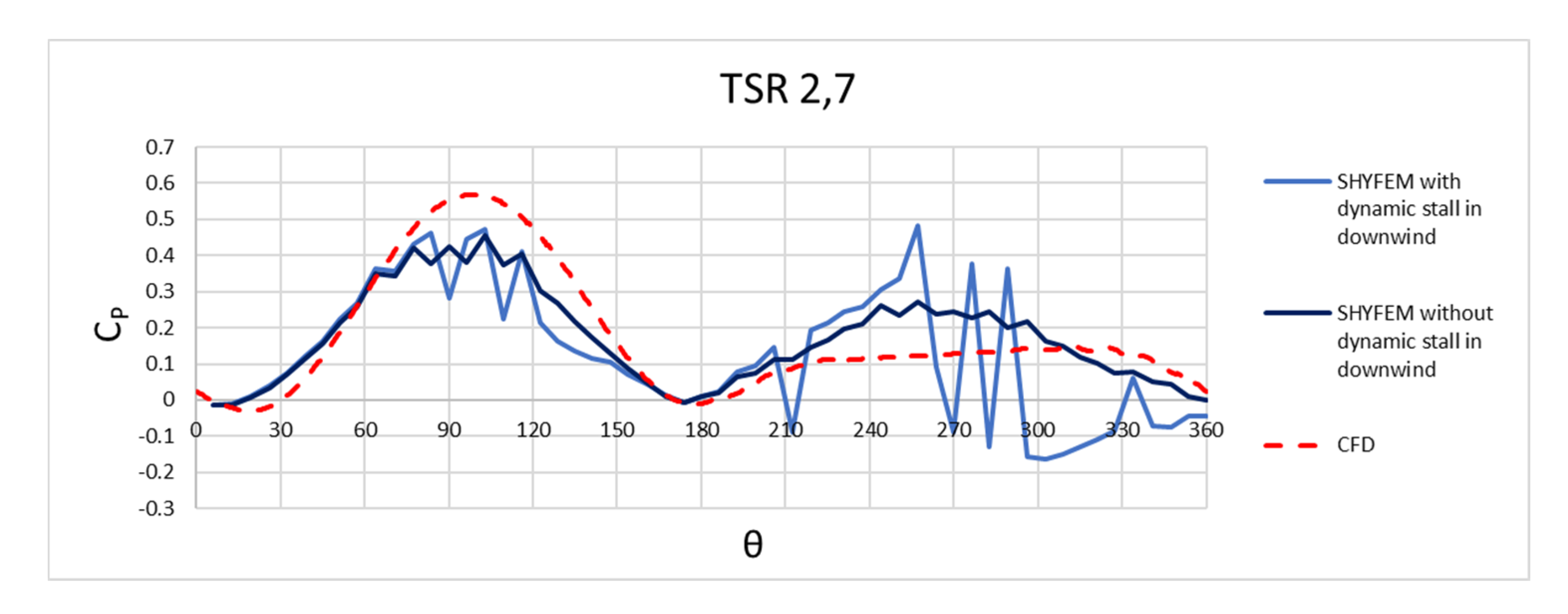
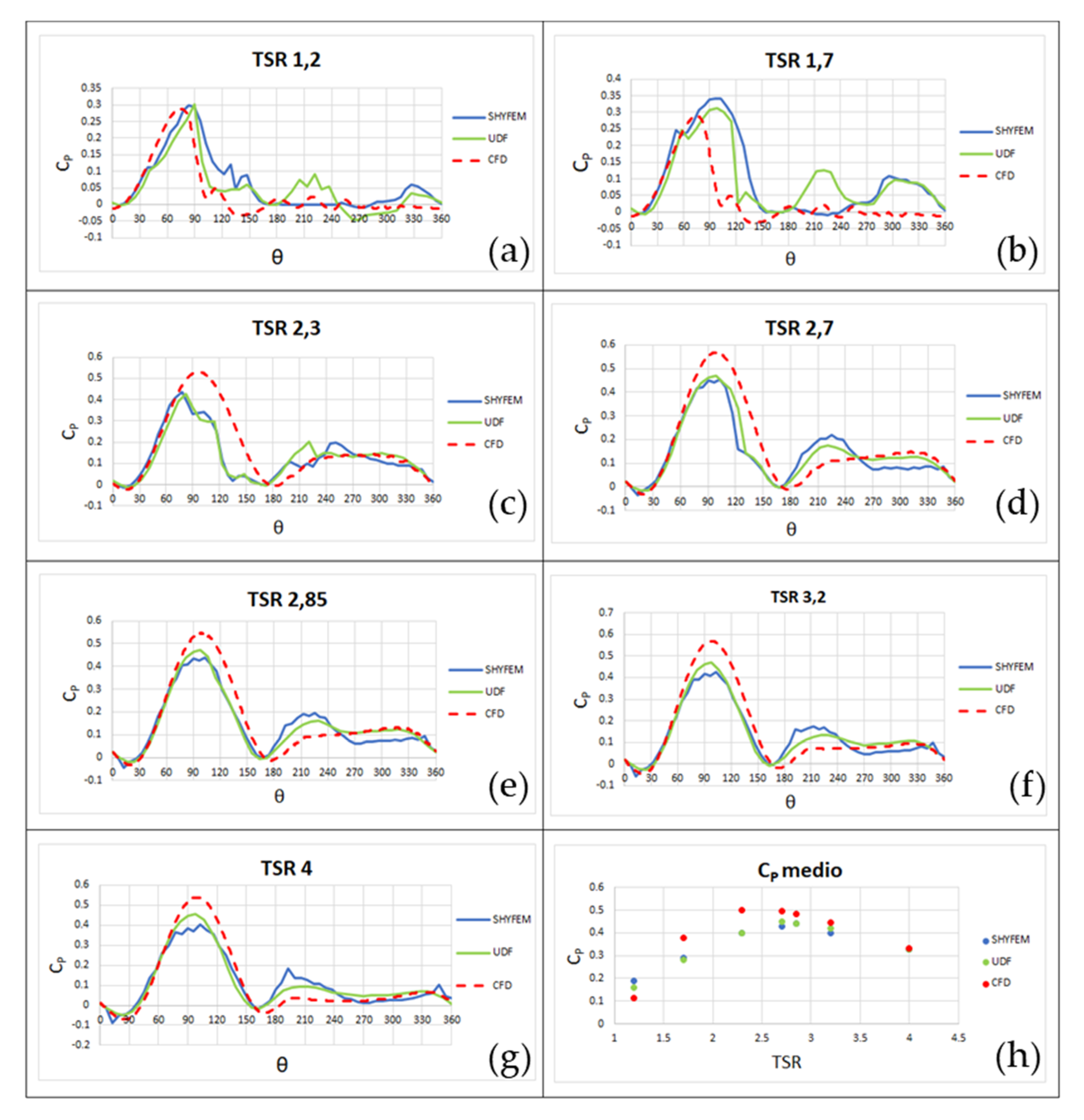
3.1. Behavior of the Single Turbine at Different TSR

Several simulations have been performed at different TSR, which were obtained by varying the rotational speed of the turbine and maintaining the free stream velocity fixed to 1.75 m/s. Other important setups are listed in

Table 2. SHYFEM setups.

Time Step (idt)	1 s
End Simulation Time (itend)	1500 s
Flow	1680 m3/s
Friction	Ireib 5 czdef 0.02
External Forces	NO

.

The results obtained with SHYFEM are very close to those obtained with ANSYS’s UDF, as shown in Figure 13. The behavior of the turbine is reported for different TSRs. It is noteworthy that not only the turbine overall C_P sufficiently matches the respective CFD result for all the TSR, but also the behavior of blade instantaneous C_P satisfies the typical azimuthal evolution in CFTs, showing, for instance, dynamic stall in upwind at very low TSR and power output decreasing in downwind as the TSR increases. What emerges is a quantitative difference between the two hybrid models and the pure CFD: as explained before, this is due to the fact that the model developed in [35] is tuned for an airfoil with lower solidity. We report also the ANSYS hybrid model in graphics just to make a comparison between the two hybrid models. Since both are based on the same analytical model, the same behavior is expected. As shown in Figure 13, expectations are satisfied for all TSR. By comparing the values of the source terms in ANSYS and SHYFEM simulations (

Table 3. Source terms entity for both ANSYS and SHYFEM hybrid models.

(N/m3)		Sources x	Sources y	Total Sources	CP Averaged
TSR 1,2	UDF	16˙004	22˙582	38˙586	0.16
	SHYFEM	35˙722	1˙520	37˙242	0.19
TSR 1,7	UDF	23˙063	33˙330	56˙393	0.28
	SHYFEM	49˙795	3˙425	53˙220	0.29
TSR 2,3	UDF	29˙681	42˙803	72˙484	0.40
	SHYFEM	65˙200	7˙292	72˙492	0.40
TSR 2,7	UDF	46˙897	33˙271	80˙168	0.45
	SHYFEM	74˙618	11˙518	86˙136	0.43
TSR 2,85	UDF	35˙425	46˙865	82˙290	0.44
	SHYFEM	77˙248	12˙946	90˙194	0.44
TSR 3,2	UDF	36˙857	48˙781	85˙638	0.42
	SHYFEM	84˙372	17˙072	101˙444	0.40
TSR 4	UDF	39˙079	51˙375	90˙454	0.33
	SHYFEM	83˙242	18˙737	101˙979	0.33

), it is evident that the total source terms are similar: differences are limited to 10% (the only exception is TSR 3.2).

This guarantees that the energy balance is respected, although the friction’s ubication has been dislocated with respect to power production, as described in Section 2.5. However, it should be noted that the relative amounts of the x and y sources are significantly different in ANSYS and in SHYFEM. This is because SHYFEM uses a unique formulation for the friction term F, while in the ANSYS’s UDF, the x and y force components to be adopted in the momentum equations are calculated by correctly projecting the lift and drag along the x and y directions.

By a qualitative analysis of the flow field velocity magnitude (Figure 14), it can be seen that SHYFEM results are similar to those obtained with ANSYS’s UDF. However, in the SHYFEM hybrid model, the grid resolution around and downstream from the turbine notably affects the wake’s length and the magnitude of the flow lateral accelerations. More details will be provided in Section 3.2.

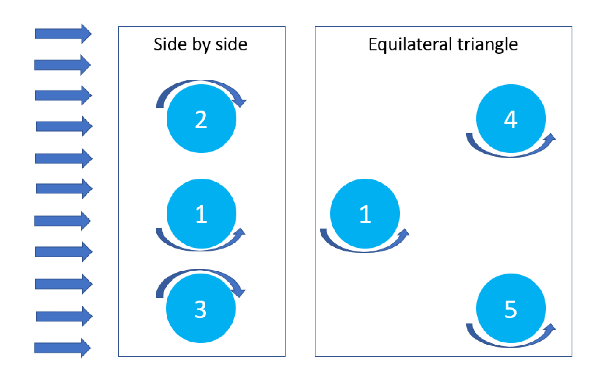
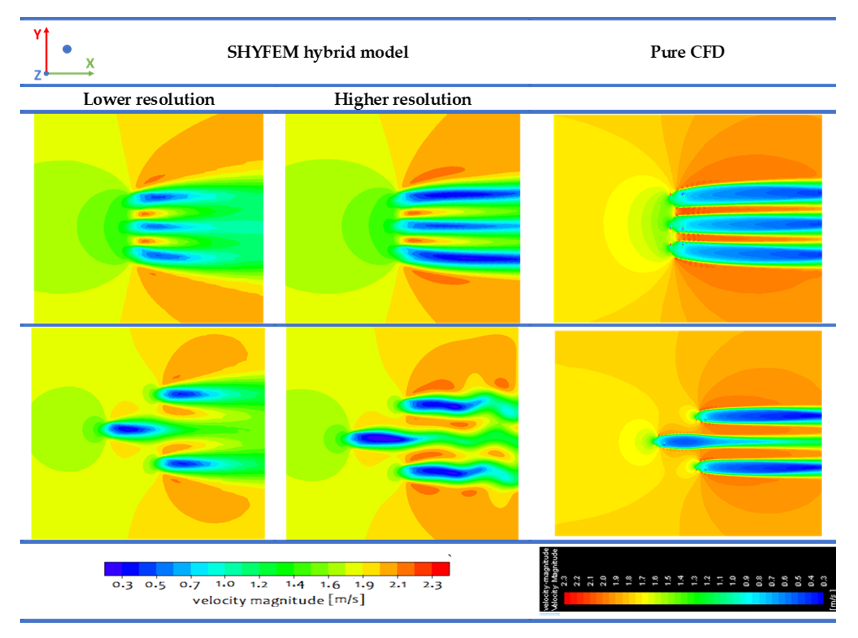
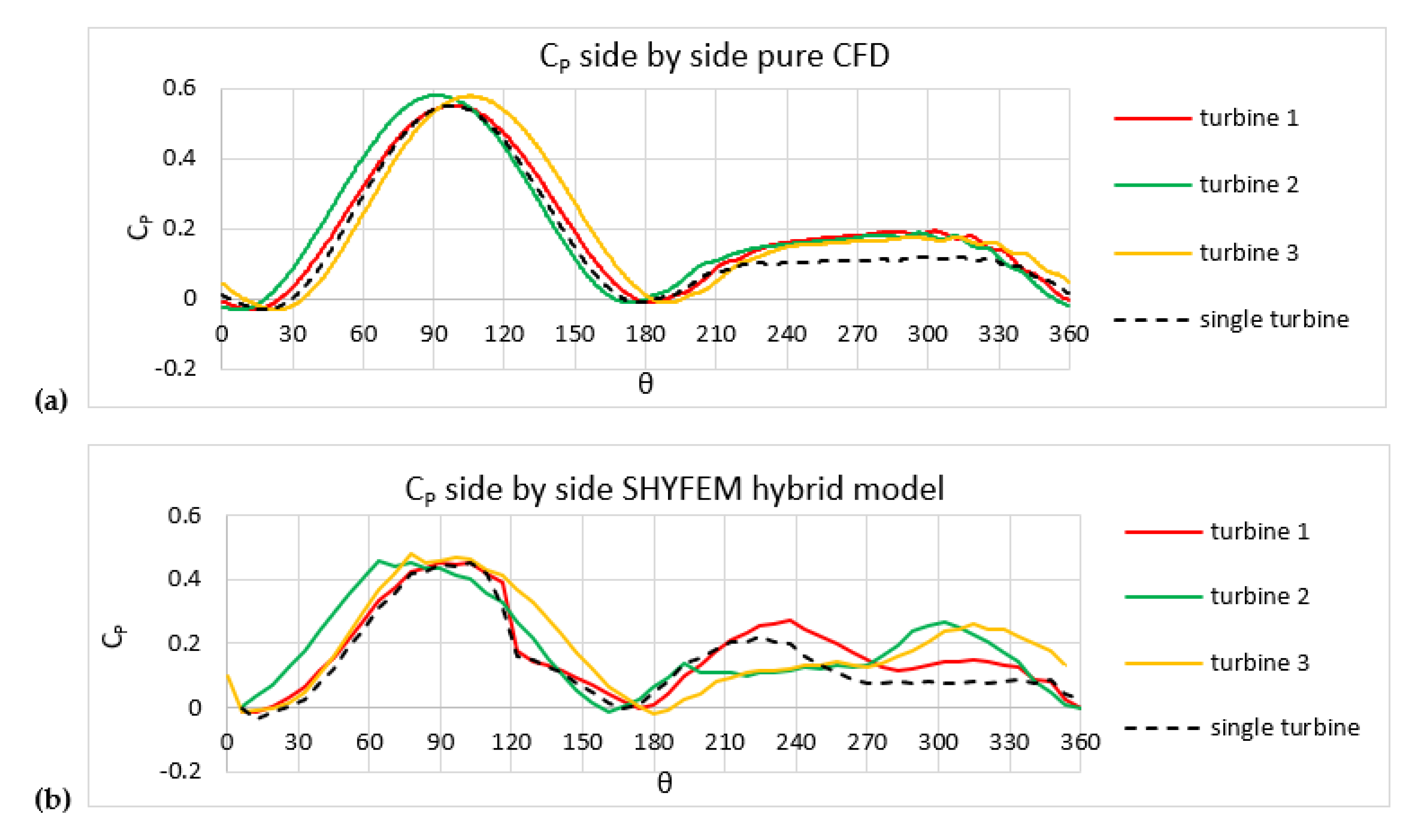
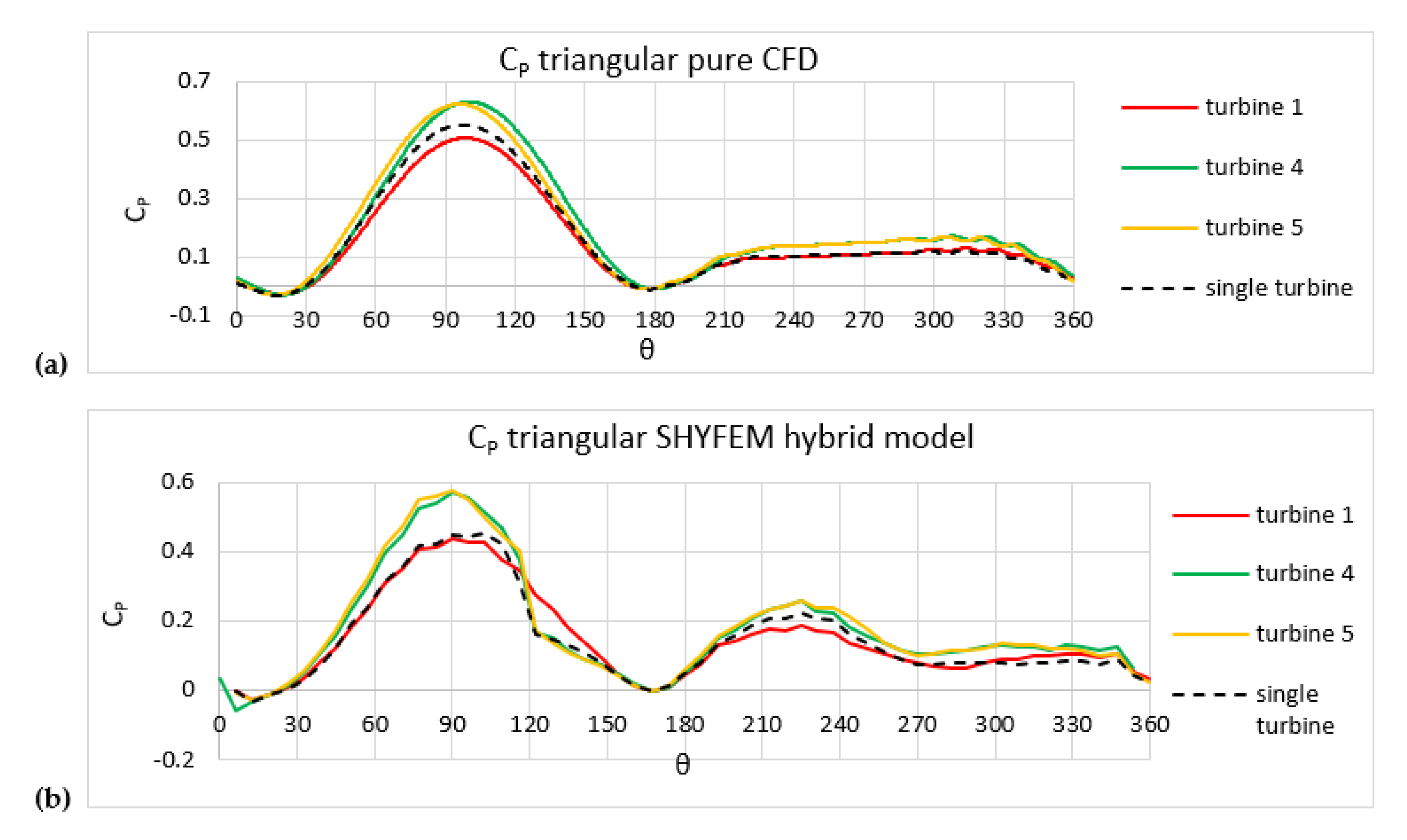
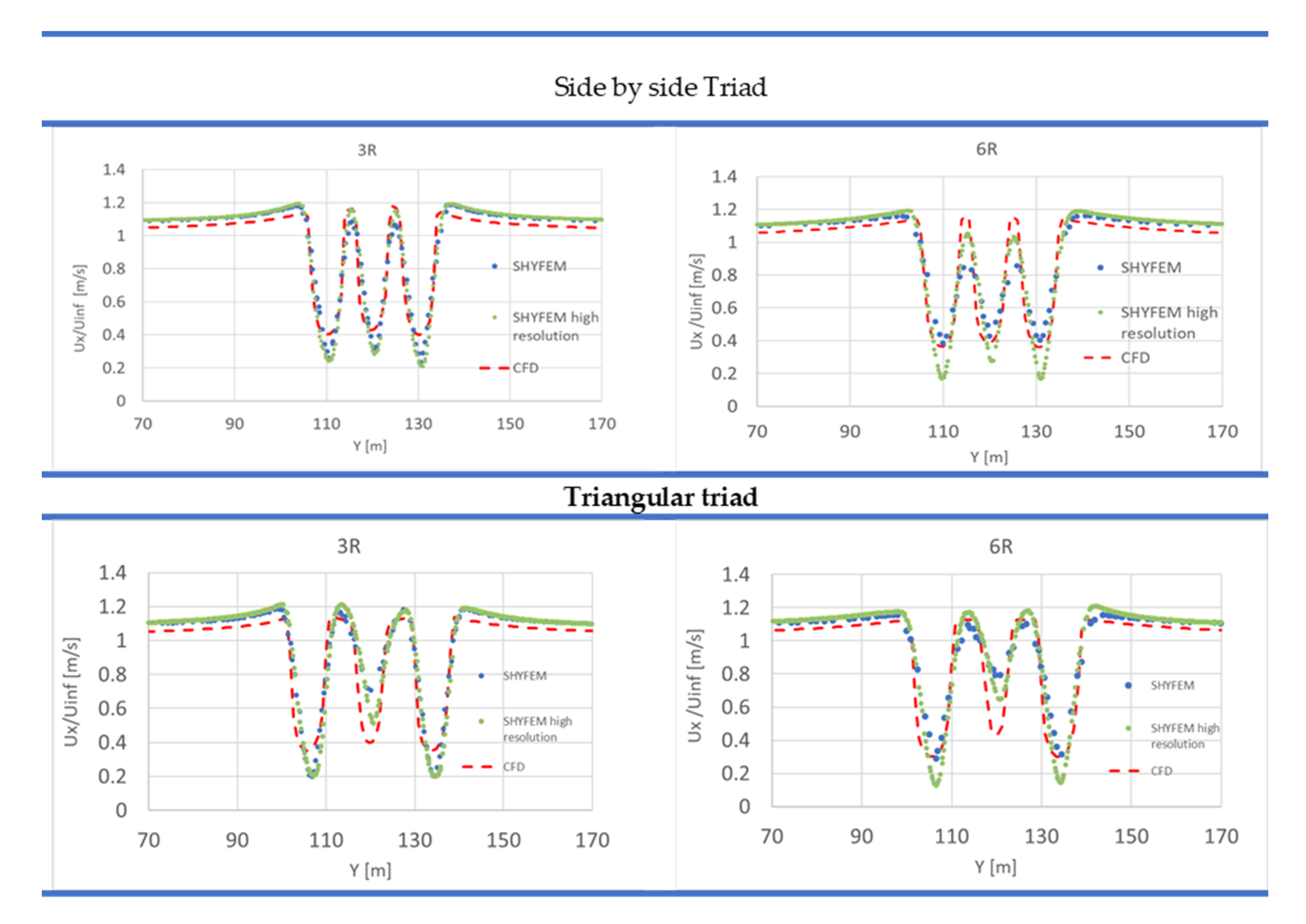
3.2. Application to a Small Turbine’s Cluster

Then, the SHYFEM model was applied to a set of three turbines in two different spatial configurations: in the first case, turbines are placed aligned with a distance between axes of 3R, while in the second case, the devices are placed at the vertices of an equilateral triangle, with distance between axes of 9.2R, as sketched in Figure 15. In this analysis, two different kinds of grid were used: one with uniform resolution all over the domain fixed at 1/6R and the other with variable resolution from about 1/6R in the turbine zone to 4/3R at the boundaries. The extension of these grids was increased to 100R along x and 80R along y (300 m and 240 m long x and y respectively) to avoid boundary blockage effects.

Figure 16 shows the flow field obtained with SHYFEM: it can be noticed, as mentioned before, how grid resolution affects the flow field. Higher resolution grids allow better visualizing velocity gradients concentrated in limited areas; furthermore, the wake length increases. This happens for both spatial configurations.

For the aligned triad, acceleration corridors appear between turbines, since the flow cannot expand freely; therefore, there is a decrease in the y component of speed and consequently also an increase in the angle of attack. The higher velocities together with the greater attack angles lead to significantly greater performance, where the acceleration corridors are located with respect to the blade path: considering turbine 1, acceleration corridors are located on both sides; this means at the beginning and at the end of upwind path for this turbine, this leads to a larger upwind C_P curve than in the isolated case, as confirmed in Figure 17. For turbines 2 and 3, acceleration corridors are present respectively at the beginning and at the end of upwind path. In fact, in Figure 17, it is shown that turbine 2 anticipates the production, while turbine 3 postpones production with respect to the isolated turbine. The behavior of the three turbines is in accordance with pure CFD results. Turbines 2 and 3 have clockwise rotational verse: in this case, the θ reference system is not the same as that proposed in Figure 5a but it is opposite with respect to the y axis. The direction of increase of the angle θ is concordant with the direction of rotation.

Instead, the higher production recorded in downwind for all three turbines is due to the fact that wakes are not free to expand; therefore, speeds in wake are higher compared to the isolated turbine case. In fact, if the wake is constrained by the presence of other devices’ wakes, the section of the stream tube is reduced, and consequently, higher velocity is recorded. In this way, the mass balance is respected.

For the triad in a triangular configuration, the incoming flow speed and then the power output are reduced for turbine 1 (Figure 18) due to the greater fluid dynamic resistance offered to the flow by the triad compared to the single device. Turbines 4 and 5, on the other hand, increase power generation in upwind, since the accelerated water flowing laterally to turbine 1 is projected onto the side turbines, which therefore benefit from higher flow velocities. The triangular triad in pure CFD simulations shows the same behavior.

In

Table 4. Percentage changes in the performance of triads.

%	SHYFEM Hybrid	Pure CFD
Turbine 1 (side by side)	17.75	17.53
Turbine 1 (triangular)	0.78	−5.97
Turbine 2	25.62	19.76
Turbine 3	28.81	18.37
Turbine 4	21.93	20.71
Turbine 5	24.95	19.37
Side by side triad	24.06	18.55
Triangular triad	15.89	11.37

, the percentage variations in performance for each single device making part of the triad, compared to the same device working alone and the performance changes for the entire cluster are presented. The results show a qualitative trend similar to the pure CFD behavior. The major quantitative differences are recorded for the side-by-side triad devices.

Wake velocity profiles are well reproduced by the SHYFEM hybrid model compared to pure CFD simulations, as shown in Figure 19. The influence of the resolution is more evident at a distance of 6R behind the turbine for both spatial configurations of turbines: this is because at 3R, the two grids still have comparable resolution, while at 6R, the difference is greater. At 3R in SHYFEM, the flow is slowed down too much, which is in accordance to the higher entity of x source terms (as shown in Table 3). The resolution affects the results at a distance of 6R where the higher resolution grid has a slower wake recovery and exhibits more distant behavior than pure CFD. It is useful to remark that these are 2D simulations: in this case, wakes are much longer compared to 3D wakes because 2D simulations do not allow vertical advection, which supports the re-energization of the wake [44]. Since 3D wakes will be shorter [13], the area where it will be necessary to have high resolution behind the turbine will be limited. Resolution has more importance in 2D than in 3D. Therefore, for all the above considerations, it can be concluded that it is not necessary to have high resolution all over the domain in order to simulate the turbine effect on the surrounding flow field. This allows enormous time savings in computing time.

It should be remarked that our current 2D SHYFEM hybrid model is similar to having a single layer to analyze, in which the depth is equal to the turbine height; consequently, none of the following 3D phenomena can be considered: accelerations of the flow above and below the turbine due to vertical blockage, vortices at the blade tips, mixing with re-energization of the wake by vertical convection. Although this limitation allows matching the results from pure 2D CFD simulations (since in those cases, it is similar to carrying out the calculations on the mid plane of a turbine with blades so long as the effects of fluid dynamic tip losses are avoided), it prevents the application of the hybrid model to identify the optimal layouts for turbine clusters. As future work, we plan to extend the embedding of the BEM model to 3D. In realistic 3D simulations, in which the water column extends above and below the turbine, the friction method should be replaced with a methodology capable of reproducing the accelerations above and below the turbine (vertical blockage). To this end, it will be necessary to evaluate whether to switch to the “source terms” method [28]. Some studies in fact show that for a horizontal axis turbine, there are no major differences in using a 3D with “source terms” or a 2D with “Bed friction” if preliminary 3D simulations are made in order to calculate the integrated average speed [49].

4. Conclusions

The Blade Element turbine analytical model for cross-flow turbines developed for SHYFEM allows obtaining results close to the pure CFD, and to the hybrid BEM-CFD model previously implemented in the ANSYS-Fluent software, yet with much lower computational effort and therefore with considerable time savings. To have an order of magnitude SHYFEM, the simulation time for a single device is about 10 min, having a set simulation end time of 1500 s, while for a small cluster of turbines, the simulation time is about 8 h with the same simulation end time. A pure CFD simulation with three rotors and the same domain extension requires about 7 days, so calculation of the time savings is relevant. It is possible to reach these results thanks to grid local refinements that are of the same order of magnitude of the finest ones nowadays adopted by other researchers using the Actuator Disc approach. Yet, in our model, turbine geometry and rotational speed are considered.

In particular, it was verified that just about 50 triangular elements on the annular ring swept by the blades are enough to reproduce even the evolution of the instantaneous C_P of the blade during a turbine revolution. This correspond to cell sizes of about 1/17 of the turbine diameter. The SHYFEM hybrid model matches the results of the pure CFD and ANSYS hybrid model also in a wide range of TSR values.

Furthermore, considering the total amount of the source terms, they differ slightly (about 10%) from the results obtained with the ANSYS hybrid model at various TSR: this ensures that although the power generation area has been decoupled from the application of the friction in the turbine-dependent friction approach, the energy balance is in any case respected.

The sensitivity analysis to the grid refinement highlights the necessity of having an adequate resolution in the turbine area and in the wake region, since C_P and the turbine effects on the surrounding and on the downstream flows depends on grid spacing.

The hybrid BEM-SHYFEM model was applied to a cluster of three turbines in two different arrangements: the results are qualitatively close to those obtained with pure CFD simulations, in terms not only of C_P increasing/decreasing with respect to the isolated turbine, but also regarding the local mutual interactions between the devices. This is not trivial, given the highly asymmetrical behavior of CFTs with respect to the plain passing through the turbine axis and parallel to the current.

After this first preliminary study, the hybrid BEM-SHYFEM model for cross-flow turbines will be adapted for 3D simulations in order to also describe crucial 3D mechanisms such as blade tip losses, vertical blockage, vertical advection, and wake recovery. The aim is to implement a tool that is useful to plan optimal layouts of tidal turbines, with the dual purpose of maximizing the mechanical energy production and minimizing the environmental effects in terms of hydrodynamic impact and turbulence generation. The difference from current studies is that it will be possible to embed turbines in real-life applications and the flow field thanks to the ability of SHYFEM to describe bathymetry, currents, tides, and surface waves as they occur in actual operating conditions. Turbines will be surrounded by a realistic flow field as if they were placed in a real area of interest; by means of the hybrid model, which is able to capture not only the average power generation of the turbine but the exact behavior of a single blade during its rotation, it will be possible to make accurate studies about energy harvested from these devices and their impact on the flow field.

References

1. Coles, D.; Blunden, L.; Bahaj, A.S. Assessment of the energy extraction potential at tidal sites around the Channel Islands. Energy 2017, 124, 171–186. [Google Scholar] [CrossRef]
2. Thiebot, J.; du Bois, P.B.; Guillou, S. Numerical modeling of the effect of tidal stream turbines on the hydrodynamics and the sediment transport e Application to the Alderney Race (Raz Blanchard), France. Renew. Energy 2015, 75, 356–365. [Google Scholar] [CrossRef]
3. Piano, M.; Ward, S.; Robins, P.; Neill, S.; Lewis, M.; Davies, A.; Powell, B.; Owen, A.W.; Hashemi, R. Characterizing the Tidal Energy Resource of the West Anglesey Demonstration Zone (UK), Using TELEMAC-2D and Field Observations. In Proceedings of the XXII TELEMAC-MASCARET Technical User Conference, Liverpool, UK, 15–16 October 2015; pp. 195–203. [Google Scholar]
4. Murray, R.O.; Gallego, A. A modelling study of the tidal stream resource of the Pentland Firth, Scotland. Renew. Energy 2017, 102, 326–340. [Google Scholar] [CrossRef]
5. Tidal Devices. Available online: http://www.emec.org.uk/marine-energy/tidal-devices/ (accessed on 5 August 2012).
6. Pathway to EMEC. Available online: http://www.emec.org.uk/services/pathway-to-emec/technology-readiness-levels/ (accessed on 30 September 2012).
7. European Comission. LCEO Ocean Energy Technology Development Report 2018; Publications Office of the European Union: Luxembourg, 2019. [Google Scholar]
8. Ferreira, C.S.; van Bussel, G.J.W.; van Kuik, G. An Analytical Method to Predict the Variation in Performance of a H-Darrieus in Skewed Flow and Its Experimental Validation. In Proceedings of the European Wind Energy Conference (“EWEC”), Athens, Greece, 27 February–2 March 2006. [Google Scholar]
9. Orlandi, A.; Collu, M.; Zanforlin, S.; Shires, A. 3D URANS analysis of a vertical axis wind turbine in skewed flows. J. Wind. Eng. Ind. Aerodyn. 2015, 147, 77–84. [Google Scholar] [CrossRef] [Green Version]
10. Dabiri, J.O. Potential order-of-magnitude enhancement of wind farm power density via counter-rotating vertical-axis wind turbine arrays. J. Renew. Sustain. Energy 2011, 3, 043104. [Google Scholar] [CrossRef] [Green Version]
11. Zanforlin, S.; Nishino, T. Fluid dynamic mechanisms of enhanced power generation by closely spaced vertical axis wind turbines. Renew. Energy 2016, 99, 1213–1226. [Google Scholar] [CrossRef] [Green Version]
12. Zanforlin, S. Advantages of vertical axis tidal turbines set in close proximity: A comparative CFD investigation in the English Channel. Ocean Eng. 2018, 156, 358–372. [Google Scholar] [CrossRef]
13. Kinzel, M.; Mulligan, Q.; Dabiri, J.O. Energy exchange in an array of vertical-axis wind turbines. J. Turbul. 2012, 13, N38. [Google Scholar] [CrossRef]
14. Van Der Molen, J.; Ruardij, P.; Greenwood, N. Potential environmental impact of tidal energy extraction in the Pentland Firth at large spatial scales: Results of a biogeochemical model. Biogeosciences 2016, 13, 2593–2609. [Google Scholar] [CrossRef] [Green Version]
15. Yang, Z.; Wang, T. Numerical Models as Enabling Tools for Tidal-Stream Energy Extraction and Environmental Impact Assessment. In Proceedings of the ASME 35th International Conference on Ocean, Offshore and Arctic Engineering, Busan, Korea, 19–24 June 2016. [Google Scholar]
16. Shields, M.A.; Dillon, L.J.; Woolf, D.K.; Ford, A.T. Strategic priorities for assessing ecological impacts of marine renewable energy devices in the Pentland Firth (Scotland, UK). Mar. Policy 2009, 33, 635–642. [Google Scholar] [CrossRef]
17. Sudderth, E.A.; Lewis, K.C.; Cumper, J.; Mangar, A.C.; Flynn, D.F.B. Potential Environmental Effects of the Leading Edge Hydrokinetic Energy Technology; U.S. Department of Energy Advanced Research Projects Agency–Energy: Washington, DC, USA, 2017.
18. Roche, R.C.; Walker-Springett, K.; Robins, P.; Jones, J.; Veneruso, G.; Whitton, T.A.; Piano, M.; Ward, S.; Duce, C.; Waggitt, J.; et al. Research priorities for assessing potential impacts of emerging marine renewable energy technologies: Insights from developments in Wales (UK). Renew. Energy 2016, 99, 1327–1341. [Google Scholar] [CrossRef] [Green Version]
19. Du Feu, R.; Funke, S.; Kramer, S.; Hill, J.; Piggott, M. The trade-off between tidal-turbine array yield and environmental impact: A habitat suitability modelling approach. Renew. Energy 2019, 143, 390–403. [Google Scholar] [CrossRef]
20. Ramírez-Mendoza, R.; Murdoch, L.; Jordan, L.; Amoudry, L.; McLelland, S.; Cooke, R.; Thorne, P.; Simmons, S.; Parsons, D.; Vezza, M. Asymmetric effects of a modelled tidal turbine on the flow and seabed. Renew. Energy 2020, 159, 238–249. [Google Scholar] [CrossRef]
21. Gillibrand, P.; Walters, R.; McIlvenny, J. Numerical Simulations of the Effects of a Tidal Turbine Array on Near-Bed Velocity and Local Bed Shear Stress. Energies 2016, 9, 852. [Google Scholar] [CrossRef] [Green Version]
22. Ramos, V.; Carballo, R.; Ringwood, J.V. Application of the actuator disc theory of Delft3D-FLOW to model far-field hydrodynamic impacts of tidal turbines. Renew. Energy 2019, 139, 1320–1335. [Google Scholar] [CrossRef]
23. Haverson, D.; Bacon, J.; Smith, H.C.M.; Venugopal, V.; Qing, X. Modelling the hydrodynamic and morphological impacts of a tidal stream development in Ramsey Sound. Renew. Energy 2018, 126, 876–887. [Google Scholar] [CrossRef]
24. Fairley, I.; Masters, I.; Karunarathna, H. The cumulative impact of tidal stream turbine arrays on sediment transport in the Pentland Firth. Renew. Energy 2015, 80, 755–769. [Google Scholar] [CrossRef] [Green Version]
25. Robins, P.E.; Neill, S.P.; Lewis, M.J. Impact of tidal-stream arrays in relation to the natural variability of sedimentary processes. Renew. Energy 2014, 72, 311–321. [Google Scholar] [CrossRef] [Green Version]
26. Schuchert, P.; Kregting, L.; Pritchard, D.; Savidge, G.; Elsäßer, B. Using coupled hydrodynamic biogeochemical models to predict the effects of tidal turbine arrays on phytoplankton dynamics. J. Mar. Sci. Eng. 2018, 6, 58. [Google Scholar] [CrossRef] [Green Version]
27. Burton, T.; Jenkins, N.; Sharpe, D.; Bossanyi, E. Wind Energy Handbook, 2nd ed.; John Wiley & Sons Inc.: Hoboken, NJ, USA, 2011. [Google Scholar]
28. Thiébot, J.; Guillou, N.; Guillou, S.; Good, A.; Lewis, M. Wake field study of tidal turbines under realistic flow conditions. Renew. Energy 2020, 151, 1196–1208. [Google Scholar] [CrossRef]
29. Michelet, N.; Guillou, N.; Chapalain, G.; Thiébot, J.; Guillou, S.; Goward Brown, A.J.; Neill, S. Three-dimensional modelling of turbine wake interactions at a tidal stream energy site. Appl. Ocean Res. 2020, 95, 102009. [Google Scholar] [CrossRef]
30. Umgiesser, G.; Canu, D.M.; Cucco, A.; Solidoro, C. A finite element model for the Venice Lagoon. Development, set up, calibration and validation. J. Mar. Syst. 2004, 51, 123–145. [Google Scholar] [CrossRef]
31. Bellafiore, D.; McKiver, W.J.; Ferrarin, C.; Umgiesser, G. The importance of modeling nonhydrostatic processes for dense water reproduction in the Southern Adriatic Sea. Ocean Model. 2018, 125, 22–38. [Google Scholar] [CrossRef]
32. Umgiesser, G.; Ferrarin, C.; Fivan; Bajo, M. SHYFEM-Model/Shyfem: Stable Release 7.4.1; Version VERS_7_4_1; Zenodo: Meyrin, Switzerland, 2018; Available online: http://doi.org/10.5281/zenodo.1311751 (accessed on 13 July 2018).
33. Letizia, S.; Zanforlin, S. Hybrid CFD-source Terms Modelling of a Diffuser-augmented Vertical Axis Wind Turbine. Energy Procedia 2016, 101, 1280–1287. [Google Scholar] [CrossRef]
34. Shamsoddin, S.; Porté-Agel, F. A Large-Eddy Simulation Study of Vertical Axis Wind Turbine Wakes in the Atmospheric Boundary Layer. Energies 2016, 9, 366. [Google Scholar] [CrossRef]
35. Rocchio, B.; DeLuca, S.; Salvetti, M.; Zanforlin, S. Development of a BEM-CFD tool for Vertical Axis Wind Turbines based on the Actuator Disk Model. Energy Procedia 2018, 148, 1010–1017. [Google Scholar] [CrossRef]
36. Mendoza, V.; Chaudhari, A.; Goude, A. Performance and wake comparison of horizontal and vertical axis wind turbines under varying surface roughness conditions. Wind Energy 2019, 22, 458–472. [Google Scholar] [CrossRef]
37. Grondeau, M.; Guillou, S.; Mercier, P.; Poizot, E. Wake of a Ducted Vertical Axis Tidal Turbine in Turbulent Flows, LBM Actuator-Line Approach. Energies 2019, 12, 4273. [Google Scholar] [CrossRef] [Green Version]
38. Shamsoddin, S.; Porté-Agel, F. Effect of aspect ratio on vertical-axis wind turbine wakes. J. Fluid Mech. 2020, 889. [Google Scholar] [CrossRef]
39. ANSYS. Available online: https://www.ansys.com/about-ansys (accessed on 1 June 2018).
40. Bravo, R.; Tullis, S.; Ziada, S. Performance Testing of a Small Vertical-Axis Wind Turbine. In Proceedings of the 21st Canadian Congress of Applied Mechanics CANCAM, Toronto, ON, Canada, 3–7 June 2007. [Google Scholar]
41. Zanforlin, S.; DeLuca, S. Effects of the Reynolds number and the tip losses on the optimal aspect ratio of straight-bladed Vertical Axis Wind Turbines. Energy 2018, 148, 179–195. [Google Scholar] [CrossRef]
42. Coiro, D.; Nicolosi, F.; De Marco, A.; Melone, S.; Montella, F. Flow Curvature Effect on Dynamic Behavior of a Novel Vertical Axis Tidal Current Turbine: Numerical and Experimental Analysis. In Proceedings of the OMAE2005: 24th International Conference on Offshore Mechanics and Arctic Engineering, Halkidiki, Greece, 12–17 June 2005. [Google Scholar] [CrossRef] [Green Version]
43. Rocchio, B.; Chicchiero, C.; Salvetti, M.V.; Zanforlin, S. A simple model for deep dynamic stall conditions. Wind. Energy 2020, 23, 915–938. [Google Scholar] [CrossRef]
44. Bachant, P.; Wosnik, M. Characterising the near-wake of a cross-flow turbine. J. Turbul. 2015, 16, 392–410. [Google Scholar] [CrossRef]
45. Migliore, P.G.; Wolfe, W.P.; Fanucci, J.B. Flow Curvature Effects on Darrieus Turbine Blade Aerodynamics. J. Energy 1980, 4, 49–55. [Google Scholar] [CrossRef]
46. Ferrarin, C.; Cucco, A.; Umgiesser, G.; Bellafiore, D.; Amos, C.L. Modelling fluxes of water and sediment between Venice Lagoon and the sea. Cont. Shelf Res. 2010, 30, 904–914. [Google Scholar] [CrossRef] [Green Version]
47. Ferrarin, C.; Umgiesser, G.; Roland, A.; Bajo, M.; De Pascalis, F.; Ghezzo, M.; Scroccaro, I. Sediment dynamics and budget in a microtidal lagoon—A numerical investigation. Mar. Geol. 2016, 381, 163–174. [Google Scholar] [CrossRef]
48. Coles, D.; Blunden, L.; Bahaj, A.S. Experimental validation of the distributed drag method for simulating large marine current turbine arrays using porous fences. Int. J. Mar. Energy 2016, 16, 298–316. [Google Scholar] [CrossRef] [Green Version]
49. Thiébot, J.; Guillou, S.; Nguyen, V.T. Modelling the effect of large arrays of tidal turbines with depth-averaged Actuator Disks. Ocean Eng. 2016, 126, 265–275. [Google Scholar] [CrossRef]
Figure 1. ANSYS-Fluent CFD CP-TSR curve vs. experimental data, concerning tests in a wind tunnel performed at a flow speed of 10 m/s. TSR: Tip Speed Ratio.
Jmse 08 01010 g001
Figure 2. (a) Grid detail in rotor zone and (b) zoom on the leading edge of the hydrofoil.
Jmse 08 01010 g002
Figure 3. (a) Schematic representation of the blade element and (b) the forces acting on it.
Jmse 08 01010 g003
Figure 4. (a) Sketch of the Kobold turbine; (b) detail of the ANSYS grid with 44 elements on the ring.
Jmse 08 01010 g004
Figure 5. (a) Scheme of upwind and downwind path; (b) CP for a single blade at different resolution.
Jmse 08 01010 g005
Figure 6. Wake velocity profile at 2R, (a) x velocity and (b) y velocity and at 10R behind the turbine (c) x velocity and (d) y velocity.
Jmse 08 01010 g006
Figure 7. CP at different TSR for both pure CFD (a) and the ANSYS hybrid model (b).
Jmse 08 01010 g007
Figure 8. Qualitative equivalence between (a) CFD symmetrical airfoil and hybrid model with virtual camber and (b) CFD cambered airfoil and hybrid model without virtual camber.
Jmse 08 01010 g008
Figure 9. SHYFEM grid details in turbine zone (a) and in a wider area around turbine zone (b).
Jmse 08 01010 g009
Figure 10. CP comparison between pure CFD and SHYFEM hybrid model with and without dynamic stall model in downwind.
Jmse 08 01010 g010
Figure 11. Qualitative scheme for assigning θ value (a) to upwind inside elements and (b) to downwind inside elements.
Jmse 08 01010 g011
Figure 12. Qualitative scheme for chord individuation.
Jmse 08 01010 g012
Figure 13. CP comparison between pure CFD, ANSYS, and SHYFEM hybrid models at different TSR values 1.2, 1.7, 2.3, 2.7, 2.85, 3.2, 4 respectively in (ag) and the averaged CP in figure (h).
Jmse 08 01010 g013
Figure 14. Qualitative flow field detail for (a) the ANSYS hybrid model and (b) the SHYFEM hybrid model.
Jmse 08 01010 g014
Figure 15. Arrangement of turbines in the two considered configurations (top view); the flow is flowing from left.
Jmse 08 01010 g015
Figure 16. Flow field comparison between the SHYFEM hybrid model, at two different grid resolutions, and pure CFD (top view).
Jmse 08 01010 g016
Figure 17. CP for the side-by-side triad both for the pure CFD (a) and SHYFEM hybrid model (b).
Jmse 08 01010 g017
Figure 18. CP for the triangular triad both for the purse CFD (a) and SHYFEM hybrid model (b).
Jmse 08 01010 g018
Figure 19. Wake velocity profile at 3R and 6R behind the turbine.
Jmse 08 01010 g019