1. Introduction
Tidal currents energy is one of the most promising offshore renewable resources in Europe. It has important advantages with respect to wind or wave power, such as minimal visual impact and perfect predictability, and it offers important attractiveness to power distribution and supply companies. To exploit tidal energy, horizontal or vertical axis hydrokinetic turbines can be used, which share with the wind turbines the operating principle and the need to reduce the investment costs in order to be configured in multi-device arrangements. To increase the power density of tidal turbine farms, the devices should be placed close to each other as possible, the limit being the avoidance of excessive hydrodynamic interference between them, which would lead to a deterioration in performance. For this purpose, experiments, theoretical models, and Computational Fluid Dynamics (CFD) play important and complementary roles of investigation and prediction.
In recent years, a number of experimental campaigns have been done with the aim of deeply understanding the physical mechanisms of interaction and identifying optimal distances between machines [
1,
2,
3,
4,
5]. Since it would be of great practical use to verify the behavior of turbines in operating conditions as close to those of the real marine environment, some of these experimental studies also include the presence of surface waves [
6]. However, the need to operate in conditions such as to guarantee the independence of the results from the Reynolds number (and therefore to use devices on a not too small scale), together with the deployment of more devices and the relatively moderate width of the test channels, often lead to the occurrence of high blockage, which could affect the results, making them unreliable if extrapolated to full-scale conditions. Although some theoretical and semi-empirical corrections are present in literature [
7,
8,
9,
10,
11,
12], some of which are based only on the value of the blockage ratio (turbine cross-sectional area divided by the channel section), others are characterized by varying degrees of complexity, and those relations are quite reliable only if applied to a single turbine located not too far from the center of the cross-section of the wind tunnel or water channel, since they have not been developed for groups of turbines nor do they take into account large asymmetries in the distances of the turbine with respect to the walls of the channel.
At full scale, the effects of the proximity of channel walls [
13] and free surface [
14], and the main interactions between the devices belonging to arrays (such as the mutual blockage) can be described by theoretical models [
15,
16]. Alternatively, the CFD, provided that the numerical model is accurately validated, is nowadays considered an effective mean to deepen the knowledge acquired through experimentation, since the simulations can be performed by geometrical scales, computational domains, and operating conditions that are not subject to constraints. Yet, despite the huge progress occurred in the computer performance, fully 3
D CFD investigations (i.e., blade resolving) requires very high computational costs and resources, which are affordable to predict the behavior of a single turbine in a few operating conditions but that are generally not compatible with extensive optimization analyses, such as the study of turbine clusters or turbines working under transient conditions such as current and waves, carried out in a reasonable time. To overcome these drawbacks, during the last decade, a few lower fidelity numerical approaches have been developed, named hybrid Blade Element Momentum theory (BEM)-CFD models, in which the turbine effect is simulated by introducing negative source terms in the momentum balance for the only region affected by the rotation of the blades. Their complexity and accuracy can be very high in case of the still highly demanding Actuator Line models; however, they appear reasonable and of appreciable practical utility in case of the Actuator Disc models, since it is widely used to simulate wind and tidal farms by adopting coarse grids with cell sizes that in some cases have dimensions comparable to the turbine diameter [
17].
At an intermediate accuracy level between Actuator Line and Actuator Disc hybrid approaches, there is the Virtual Blade Model (VBM), which is an implementation of the Blade Element Momentum theory (BEM) within the commercial software ANSYS Fluent. Briefly, the VBM is a turbine analytical model based on the Blade Element formulation; in fact, it describes the forces that are generated by the interaction between the flow and blade at a particular radial position considering the blade geometry. This is possible, since the turbine disc is discretized in a few thousands cells. Embedding the VBM in a CFD code means making a type of two-way coupling, in which the information transmitted from the CFD to the VBM are the local conditions of the flow, while the information transmitted from the VBM to the CFD code are source terms for the momentum equations, corresponding to the aforementioned forces. Then, the main difference with a purely analytical BEM approach is that the part concerning the Momentum Theory is directly solved by the CFD code. Yet, different to the embedding of an Actuator Disc model, the turbine performance coefficients are not input of the problem, but they are calculated on the base of the operating conditions and blade geometry. The VBM, originally developed by Zori and Rajagopalan [
18] for applications on helicopter rotors, has already proved to be a valuable tool to predict not only the performance coefficients and wake characteristics of a wind turbines single rotor [
19] and turbine arrays also in misaligned flow conditions [
20], but also the behavior of a tidal turbine subjected to waves [
21,
22]. In our study, the VBM is used to investigate the interaction between two horizontal axis tidal turbines (HATTs) arranged in line and working under combined conditions of tidal current and surface waves. The objective was to try to answer to these questions:
“How much does the performance achieved for a small-scale turbine in a relatively narrow channel change when a scaling-up to an unconfined environment is done?”, and
“Is a low-fidelity BEM-CFD approach adequate to capture both the power/thrust coefficients and also the wake evolution details?”, and finally,
“Could the VBM be used as an aid to the laboratory scale experimentation in order to take into account the blockage effects before to extend the results to full scale applications?” 2. Numerical Method
2.1. Virtual Blade Model
The turbine has been modeled according to the hybrid BEM-CFD Virtual Blade Model, which was implemented on ANSYS Fluent by means of a User-Defined Function (UDF). A UDF is a function written by the user in the C programming language that can be dynamically loaded with the solver to enhance the standard features of the CFD code. The VBM simulates the effects of blade rotation through the introduction of momentum source terms that act within a fluid disk with an area equal to the swept area of the blades, without physically representing them in the computational domain. These source terms are forces in the
x,
y, and
z directions calculated using a classic BEM approach, so that the fluid inside the disk is affected by the same forces it would be interested in if the blades were present. The necessary inputs are the distribution of the chord and the twist angle along the blade, depending on the rotor design, and the lift and drag coefficients as a function of the attack angle and Reynolds number. In the present study, coefficients were obtained experimentally for the airfoil used here, and this information has been extended for different ranges of Reynolds numbers or angles of attack with the XFOIL code, which has proven to be a good tool for predicting the performance of airfoils at low Reynolds numbers [
23]. In addition, it has been shown that by using lift and drag coefficients, a good approximation can be obtained when assessing wave and current flows in tidal stream turbines [
24]. The airfoil used throughout this investigation is a Wortmann FX 63-137.
The domain of the rotor is divided into small sections in the radial direction from the hub to the tip; for each section, depending on the calculated values of the angle of attack and the Reynolds number, the lift and drag coefficients are interpolated on the basis of the tabulated coefficients. For each element, on the basis of the coefficients thus obtained, the length of the chord and the relative flow velocity, the lift and drag forces are calculated with the following formula [
25]:
where
CL,D is the drag or lift coefficient for unit span,
c is the chord,
ρ is the density of the fluid,
ξ is the normalized radial position along the blade of the section, and
Vtot is the relative flow velocity hitting that section of the blade, which is determined by the absolute speed of the flow and the rotation speed of the turbine (for the initialization of the calculation, the undisturbed flow velocity is considered).
Lift and drag forces (
FL,D cell) are averaged over a complete revolution of the turbine to calculate the source terms for each cell of the numerical discretization, as volume forces (
Scell):
where
Nb is the number of blades,
θ is the azimuthal coordinate, and
Vcell is the volume of the cell. The added mass has not been considered in these calculations, given that the Keulegan–Carpenter number is sufficiently small, as outlined by [
26].
The flow is loaded with these forces and the process is repeated until convergence is achieved. Other than that, a classic 3D RANS or URANS calculation is performed in the remaining domain, as needed. During the progress of the calculation, the User-Defined Function, at each iteration, shows in the console the obtained values of axial thrust and torque, which are calculated as the sum on the entire disk of the individual thrusts and torques acting on each cell, and the power, given by the product between torque and angular speed.
2.2. Grid
The calculation grids of the various simulations have been created through the software ANSYS ICEM and consist of multi-block structured 3
D grids, with the addition of O-grids to thicken the distribution of cells in the areas of greatest interest and at the same time to improve their quality. It is worth mentioning that structured, and then regular, grids allow obtaining more accurate results and decrease the calculation times. The rotor is represented by a circular O-grid with the thickness of one cell, as can be seen in
Figure 1a, to which is assigned the boundary condition of “interior” and not “wall”, as conventionally happens, since as already mentioned, the blades are not physically present, but source terms are applied to the fluid disk corresponding to the area swept by them. The boundary conditions assigned to the various elements are summarized in
Table 1.
The reference coordinate system is defined as
x in the streamwise,
y in the vertical, and
z in the spanwise directions, respectively. A partial representation of one of the grids used is shown in
Figure 1b.
2.3. Setup
ANSYS Fluent v19 was used to resolve the flow hydrodynamics by solving the RANS equations via the finite-volume method; the numerical calculation is of the “pressure-based” transient type. Within the software, the pressure and velocity fields are obtained from the Reynolds-averaged Navier–Stokes equations (RANS):
where
p is the total pressure,
ρ is the density of the fluid,
vi is the instantaneous flow velocity along the i-th direction,
is the fluctuation in velocity,
Fi is the external body force in the
i-th direction,
µ is the dynamic viscosity, and the over-bar denotes time-averaged quantities.
The turbulence model used for closing the equations is the k-ω SST (Shear Stress Transport), which combines the precision of the k-ε model in the free flow field with the most precise and stable formulation of k-ω in the region near the walls [
27]. A second-order solution method has been utilized for the spatial and temporal discretization. The convergence criterion imposed provides that the residues are less than 5 × 10
−5 for each quantity. The two-phase treatment has been made possible through the implementation of the Volume Of Fluid (VOF) method for modeling the free surface between the two fluids, which was originally developed by Hirt and Nichols [
28]. For each phase, a variable relating to its volumetric fraction is introduced in a given calculation cell; consequently, within each cell, the physical properties are expressed as the weighted average of the volume occupied by the individual fluid. The tracing of the free surface is made possible by solving the continuity equation for the volumetric fraction of one of the two phases, in the following form (for the
qth phase):
where
is the volumetric fraction of the
qth fluid,
is the velocity,
n is the number of phases,
S is a source term, if present,
is the mass transfer from phase q to phase
p, and vice versa,
is the mass transfer from
p to
q. This equation will not be solved for the primary phase, for which the volume fraction will be computed based on the constraint:
In addition, the activation of two VOF sub-models, “Open Channel Flow” and “Open Channel Wave BC”, allows the setting of the waves and their characteristic parameters, height
H and length
LW. The waves implemented in the present study are of the “Shallow/Intermediate Waves” type, which is typical of intermediate depths where 0.06 <
d/LW < 0.5 (
d is the depth of the channel) [
29]. Based on the Ursell number (
Ur = H·LW2/d3), which indicates the degree of non-linearity of the wave, and on the “steepness”
H/LW, it is possible to choose the most suitable analytical theory for wave modeling; the linear wave theory is indicated as satisfactory for
Ur < 40 and
H/LW < 0.04 [
30], as in the present case. The assigned wave parameter for the laboratory scale simulations, based on the wave operating conditions that will be adopted in the experimental campaign, are shown in
Table 2.
2.4. Model Validation
The first part of this work consists in validating the VBM in terms of predicting the performance of a horizontal axis tidal turbine and the wake generated by it through comparison with laboratory-scale experimental measurements. To the authors’ knowledge, it is the first time that a complete validation of the hybrid Virtual Blade Model approach for the study of a marine turbine has been carried out by comparison with experimental results. Sufian et al. [
22] completed the validation only in regard to the prediction of the wake, while Bianchini et al. [
19,
20] instead focused on the comparison with the results obtained with a traditional CFD-3
D approach regarding wind turbines.
Due to the experimental data available for the small-scale turbine that is being assessed, the validation of the performance evaluation is carried out for a 0.9 m diameter rotor, while the wake evaluation is based on a similar but smaller-scaled turbine (0.5m in diameter). However, both devices are 3-bladed horizontal axis turbines and the rotor blades are based on a Wortmann FX 63-137 airfoil. The full details of the physical devices are reported in [
31,
32,
33], but a brief description is also given in the follow sections.
2.4.1. Performance Validation
The validation in terms of performance, i.e., the verification of the correct prediction of the main quantities generated by the turbine, such as axial thrust and power, has been carried out by comparing the results of the VBM simulations with the experimental measurements carried out in [
31].
The VBM is based in the experimental campaign carried out at the CNR-INM towing tank in Rome, on a small-scale three-bladed horizontal axis turbine with a diameter of 0.9 m and fully described in [
32]. The dimensions of the tank are 9 × 3.5 × 220 m; the center of the turbine hub, towed at a constant speed of 1 m/s, was installed in the central section 1.5 m below the free surface. For the validation of the VBM, only cases of current-only have been considered, i.e., in the absence of waves, for different turbine rotation speeds.
Preliminarily, three sensitivity analysis have been performed [
34]:
Sensitivity to the fineness of the grid: a mesh with about 5000 elements inside the disc ensures reliable results without excessive calculation times.
Number of “revolutions” of the turbine necessary to reach the steady-state condition in the results: 30 revolutions are sufficient to foresee not only power and thrust but also the formation and the complete development of the wake.
Sensitivity analysis to the tabulated coefficients of lift and drag to be provided as input to the simulations, which showed that the range of angles of attack and Reynolds numbers relating to the available experimental coefficients were initially too narrow. In particular, the lack of data for large attack angles, which causes a strong increase in the drag coefficient, caused a considerable overestimation of the power produced at low Tip Speed Ratio (TSR) values. For this reason, the software XFOIL has been used to retrieve the missing data.
Once the most suitable parameters to be used were determined, simulations were carried out for 11
TSR values from a minimum of 1.5 to a maximum of 6.65. The results in terms of dimensionless power and thrust coefficients as a function of the
TSR are shown in
Figure 2 in comparison with the experimental measurements from [
31]. The
CP trend is predicted in a sufficiently correct manner, particularly in the vicinity of the peak value, where the correspondence is very good, while a certain discrepancy occurs for very high or very low
TSR values. The
CT curve matches the experimental results satisfactorily, except for the lowest
TSR value. In general, the global results (the
CP and
CT trends as a function of
TSR), but also the local results (inflow angle and attack angle distributions), have been shown to be consistent with what can be expected from the theory [
25].
2.4.2. Wake Validation
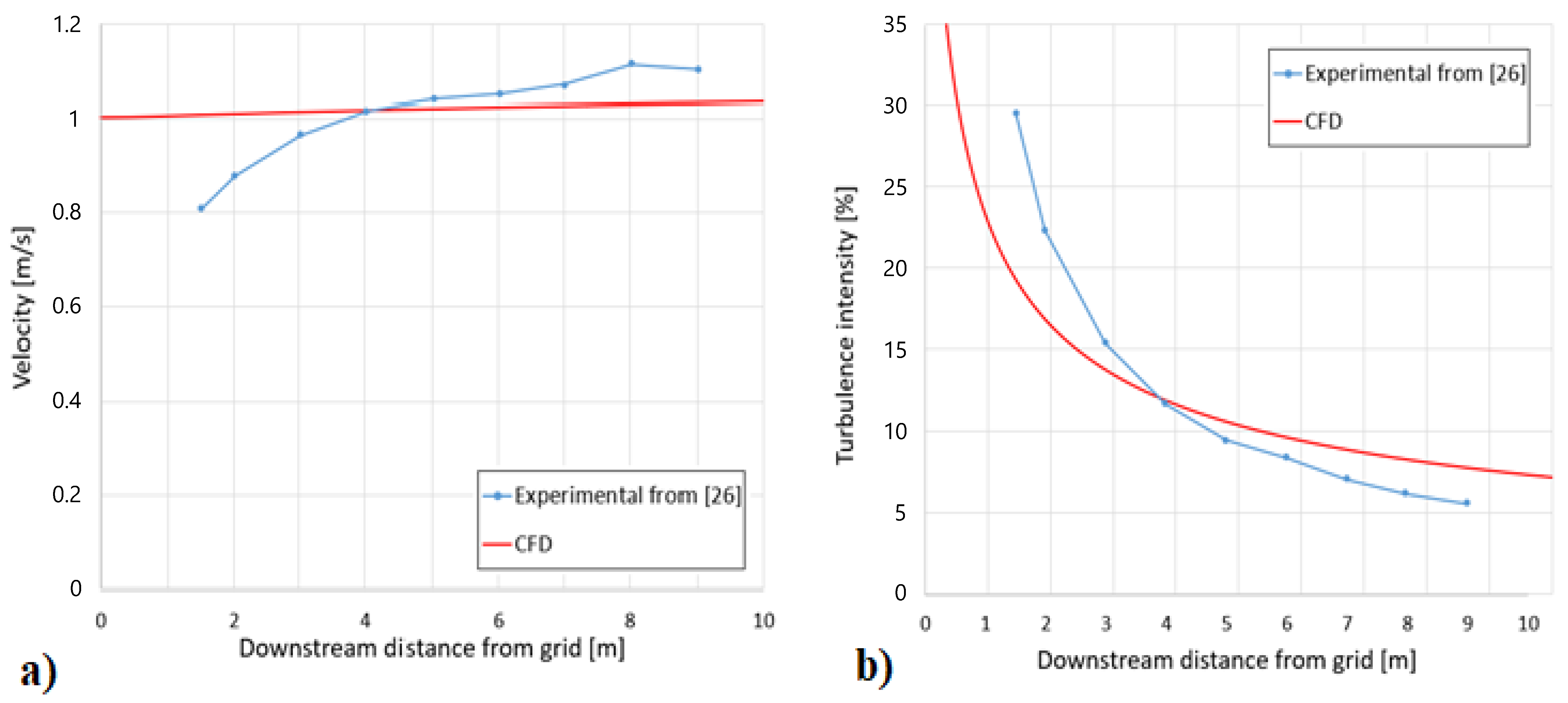
In order for a turbine model to be considered reliable, it is necessary that it provides a correct prediction of the evolution of the wake produced as well as its performance. As the experiments undertaken in [
31] do not evaluate wake evolution, the velocity profiles measured experimentally in the work done by Ebdon et al. [
33] were taken as a reference and were compared with the results provided by the VBM. The experimental campaign was carried out at the IFREMER flume tank in Boulogne-Sur-Mer, measuring 4 × 2 × 18 m, using a turbulence generating grid positioned 4 m upstream of the turbine. The reference turbine has different dimensions from that of the analysis in
Section 2.4.1, now having a diameter of 0.5 m, but the blades are made with the same airfoil (Wortmann FX 63-137); it was installed 1 m below the free surface in the central section of the tank. The wake measurements were made along the horizontal plane containing the turbine with a two-axis Laser Doppler Anemometer (LDA) system, for different positions downstream of it, for
TSRs of 2.5, 3.65 and 4.5. Preliminary measurements in the absence of the turbine detected a flow velocity of 1.02 m/s, a turbulence intensity of 11.7%, and a scale length of 0.19 m at the center of the rotor. In the computational analysis, preliminary simulations were carried out to ensure the same values at the center of the rotor; however, it was not possible to reproduce exactly the same experimental profiles of speed and turbulent intensity downstream of the grid along the centerline, as can be seen from
Figure 3.
The wakes generated at all three simulated
TSRs are in line with the theory, i.e., the phenomena of the formation, development, and dissipation of the wake are reproduced correctly. For each distance downstream of the turbine, the general shape and the width of the wake correspond to those measured experimentally, while its intensity is not always perfectly predicted, with an average accuracy of around 90%. The wake velocity profiles obtained for
TSR = 4.5 are shown in
Figure 4, in comparison with the experimental profiles from [
33]. The wake is almost perfectly reproduced for
x/D = 2, 3, 4, 7, while for
x = 5
D, the VBM underestimates the experimental results by about 5%, not capturing the rapid evolution of the wake. The failure to reproduce the flow acceleration downstream of the grid greatly influences the results especially in the far wake: in fact, at a distance of 9 and 12 diameters from the turbine, the velocity is overall underestimated by about 10%. It can also be observed that at all distances, there is an underestimation of speed in the flow outside the wake. This can be justified by the fact that experimentally, the velocity field in the absence of the turbine was slightly uneven in the lateral direction, with a slight acceleration at the sides with respect to the center, but in the absence of precise data in CFD simulations, a perfectly uniform flow was imposed with speed equal to the value measured in the center of the tank.
3. Laboratory Scale Simulations
After being validated, the VBM will be used to evaluate the interaction between two HATTs in combined conditions of waves and currents, reproducing the operating conditions of an experimental campaign that was planned for April 2020 at the IFREMER flume tank in Boulogne-Sur-Mer, but due to the COVID-19 emergency, it has been postponed. For this reason, the results obtained from the numerical simulations cannot be compared with experimental data but rather represent a preliminary analysis for future laboratory tests aimed at identifying the most interesting operating conditions in compliance with the constraints imposed by the width and length of the channel.
The turbine used is the same as that described in
Section 2.4.1, with a diameter of 0.9 m. Four conditions have been compared:
Single turbine;
Two aligned turbines (the two axes coincide);
Two turbines with a lateral cross-stream offset between the two axes of 0.75 diameters;
Two turbines with a lateral cross-stream offset between the two axes of 1.5 diameters.
Both turbines are positioned at a depth of 1 m and a distance of 3 m parallel to the direction of the current, which was set to 1 m/s in all cases. The first turbine always operates at
TSR = 4, which is equal to the peak value found in a previous campaign under similar conditions [
35], while the second has been tested at different rotation speeds, corresponding to
TSR = 2, 3, 4, 5, since it is not known a priori whether the second turbine is in the wake of the first or if on the contrary, it benefits from acceleration of the flow induced by blockage phenomena of various kinds, such as the presence of the first turbine or the effect of the proximity of the walls.
It should be noted that the
TSR is always defined with respect to the undisturbed flow measured in the case of an empty channel. This makes sense if there is only one turbine, while it is questionable in the case of in-line turbines (or back to back turbines), since the second turbine is subject to very different local speeds. However, this is a habitual choice when simulating and testing arrays of turbines [
1,
2,
36]. Similarly, the coefficients of power and thrust of the downstream turbine are still computed from the upstream velocity; then, it is important to understand that “
CP” is an abuse of notation, since it does not represent the power coefficient but it is an indicator of the power retrieved as compared to the upstream velocity. However, the good practice is to try to maximize the
CP by lowering the angular velocity and therefore the
TSR, and therefore, it has been chosen to simulate the
TSR = 2 case as well.
In order to carry out a reliable comparison with the experimental data, the domain of the fluid water region has the same height (2 m) and the same width (4 m) of the IFREMER flume tank, while in a precautionary way, the length in the direction of the current has been increased by 1D upstream and 1D downstream to allow the independence from the boundary conditions and an adequate wake development of the second turbine. Above the water region, the fluid region of air with a height of 2 m has been added.
In the experimental working section, a (1/7)th power-law boundary layer is declared in the bottom of the test section of about 30 cm height [
37]. The boundary layer is a very thin region of flow near a solid wall in which viscous forces are very important due to the no-slip boundary condition and therefore cannot be ignored. The thickness of the boundary layer is conventionally defined as the height at which the flow velocity reaches 99% of the undisturbed inlet velocity. Within the program ANSYS Fluent, in order to reproduce the boundary layer experimentally detected, a boundary condition of “no-slip wall” has been assigned to the bottom surface. The wall roughness effects have been included by setting a roughness height of 2 mm and a roughness constant of 0.5 (standard value for uniform roughness [
29]). The roughness height value has been chosen after several attempts, and it is the one that allows obtaining at the geometric end of the channel (18 m) a height of the boundary layer equal to about 0.3 m, as in the experimental conditions.
As well as in laboratory conditions, a very low background turbulence intensity of 1.5% has been set.
3.1. Effects of Turbine Offset
Analyzing the velocity field downstream of the isolated turbine (
Figure 5), it is possible to observe that where the second turbine will be positioned, the speed deficit induced in the flow is still very pronounced.
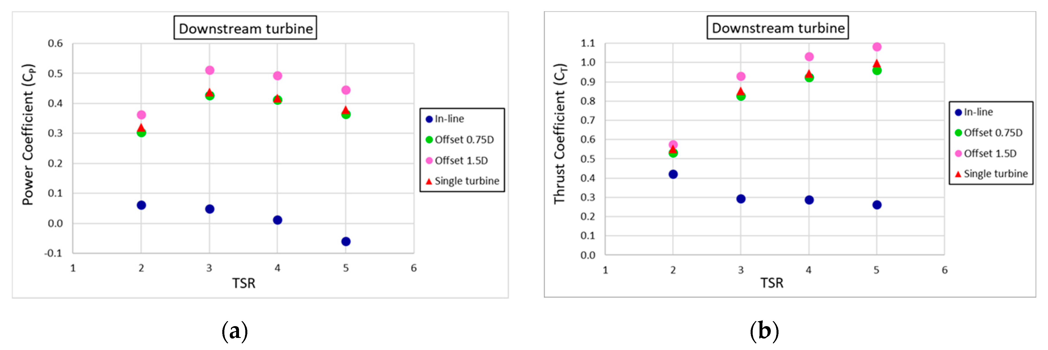
In all the cases analyzed with two coupled turbines, it has been found that the dimensionless thrust and power coefficients of the upstream turbine do not vary significantly with respect to the base case, so it can be said that it operates in the same way as an isolated turbine, which was expected and further verifies the model set-up. The performance of the downstream turbine is strongly influenced by the presence of the upstream device and their relative position. In
Figure 6, the
CP and
CT of the downstream turbine as a function of
TSR are compared with the results of a single turbine in the current-only conditions. In the “in line” configuration, both coefficients assume a monotonous decreasing trend, with the maximum for the lowest
TSR, and both the power and the thrust undergo a strong collapse compared to the base case; in particular, the power generated is always more than 80% lower. When a lateral offset is introduced, the trends of the dimensionless coefficients as a function of
TSR reflect those of the base case, with
CP having a maximum for
TSR = 3 and with an increasing monotone
CT. For the case with 0.75
D, the offset power and thrust are similar but slightly lower than the single turbine, not more than 4%, while in the case with 1.5
D offset, they are considerably higher; in particular,
CP is greater than about 13% for
TSR = 2 and more than 17% for the other three
TSR values.
The influence of the wake of the upstream turbine on the downstream device is clearly observable from the axial velocity range, as shown in
Figure 7a for the various configurations for
TSR = 4, on a horizontal plane passing for the turbines axes. When placed in line, the kinetic power available for the second turbine is very low, as it is completely undergone to the wake of the first. For this reason, the second turbine does not have its own wake; rather, it is a sort of extension of the initial wake, with an even more marked reduction in speed. However, the speed is recovered quickly, which is probably due to the strong turbulence present. In the opposite case with the 1.5
D offset, the two turbines each have their own distinct wake. It can be observed that the wake of the first device is strongly influenced by the presence of the second, undergoing a thinning in the side close to it and a strong re-energization inside, due to the acceleration induced by the latter in the channel. In the configuration with intermediate offset of 0.75
D, the downstream rotor is partially invested by the wake of the first one, so it receives a highly uneven speed profile as input. The result is a complicated interaction process where the individual wakes are initially visible, but further downstream develops what can be considered a very large single wale. It can be seen that the recovery of the second wake is very rapid.
Figure 7b displays the contours of streamwise velocity detected in correspondence of the front face of the two source term discs, for cases with two turbines, which are arranged according to a frontal view. It can be seen that the velocity field in front of the first turbine is always the same for all three configurations, while the speed profile that affects the second rotor is obviously very different, changing the lateral offset. In case B, it is hit by a uniformly very low velocity; in the opposite way, in case D, it is hit by a high velocity range, which is overall slightly greater than that which involves the upstream turbine. In case C, with a lateral offset of 0.75
D, the disc is crossed by a non-uniform speed range: on the right side, the partial influence of the wake of the upstream rotor can be clearly noticed.
In analyzing the results, attention must be paid to the onset of the blockage effect: the proximity of the turbines to the side walls, which inevitably occurs in cases with offset, prevents the flow from expanding externally, causing intense acceleration on the sides of both the devices. It is interesting to note that the second disc is, at least on the wall side, is characterized by more yellow-red colors than the first one, which is a sign that the blockage is more intense. In the case of 1.5
D offset for the downstream turbine, the colors tend more to yellow-red because it benefits from both the blockage of the walls and the blockage induced by the wake of the upstream turbine. Regarding the 0.75
D offset case, for the second turbine, the benefit of blockage of the proximity of the walls is almost eliminated by the fact that the disc is also partially hit by the wake of the first turbine. In conclusion, the phenomenon of blockage is more marked in the case with a 1.5
D offset, as clearly visible in the bottom box of
Figure 7a (case D); this entails an average higher velocity range on the downstream disc and therefore a considerable increase in thrust and generated power.
In
Section 4, the simulations will be repeated in an unconfined environment to evaluate the incidence of the effect of lateral blockage on the results.
3.2. Effects of Turbine Offset under Current-and-Wave Conditions
The wave characteristics were selected to have a height of 0.15 m and a frequency of 0.7 Hz, which results in a length of 5.6 m. These characteristics were chosen to extend the research undertaken in previous test campaigns for similar conditions but for a single turbine [
35]. These parameters are also representative from common sea states, as it can be seen in
Section 4 and in [
24]. All the models are based on regular wave conditions. Preliminary simulations in the absence of the turbine have confirmed that the passage of the wave involves important variations in the axial velocity of the flow, as it can be seen in
Figure 8, even if the average effect over a period is zero. The influence of the waves is stronger in the vicinity of the free surface, while it attenuates toward the bottom: it goes from a speed fluctuation of 34% at the upper end of the rotor disk to 15% at the lower end. From the same figure, it can be noted that since the waves are generated on the input face, their effect gradually decreases going toward the output face due to the viscosity of the water; it has been verified that between the position of the first and second turbines, being very close, there is a decrease in the intensity of the fluctuations of less than 3%.
In the presence of waves thrust, the torque and power of both turbines assume an oscillatory character, with a period equal to the wave period; the maximum values occur when the device is under a wave crest and the minimum values occur at the trough, as it happens with the axial velocity component of the flow (
Figure 8). The waves have a greater effect on the power than the thrust, since the first depends on the speed cubed, while the second depends on the speed squared. This is also the reason why in the same way the power of the downstream turbine is more affected by the influence of the upstream turbine than the thrust.
As for the average values of torque and thrust over a period, they do not change significantly compared to the corresponding cases in the absence of waves; however, in each simulated case, a slight increase in the produced average power has been measured, which is equal to a few percentage points in most cases. The only cases in which this increase becomes significant are the two with offset for
TSR = 5, in which the increase is 8.6% with an offset of 0.75
D and 5.4% with an offset of 1.5
D. The reason why, for all the TSR, the power relative gain is for the 0.75
D offset turbine is related to the wake re-energization effect induced by waves. In fact, as it can be seen on the maps obtained by averaging the velocity values for a wave period (
Figure 9a), the waves cases produce a slightly faster wake recovery. Yet this phenomenon implies a power gain only for turbines that are located in the trajectory of the wakes released from upstream turbines, since in this case, the turbine works in a flow field characterized by slightly higher velocity than in the case without waves, as justified by the less extension of the blue region on the axial velocity distribution on the source term disc in
Figure 9b for the 0.75
D offset turbine in case of waves.
However, the general results obtained in current-only conditions do not change, and the most important effect brought by the presence of the waves is not so much that on the average value but rather the induced oscillations, whose intensity becomes stronger by increasing the
TSR, as can be seen from the graph in
Figure 10, which is in line with the results of [
35].
When the downstream turbine is placed in line, the power (and thrust) oscillations become disproportionate, with values that abundantly exceed 100% of the average power, further confirming that it is preferable to avoid this configuration. In cases with offset, the fluctuations are slightly smaller than in the base case, with a greater advantage for high
TSR. A first cause of this reduction is undoubtedly the aforementioned dissipation of the waves along the domain (
Figure 8). Secondly, since the downstream turbines work in a flow field augmented by the blockage effects (walls and upstream turbine), the velocities generated by the waves are relatively less influential. Moreover, the fact that in the case with 0.75
D offset, the oscillations are smaller than in the case with 1.5
D offset, with the same position in the domain, could indicate that the interaction with the upstream wake attenuates the oscillating effects of the waves; further analysis to understand these interactions is required looking at additional permutations of lateral offsets and wave parameters, which are beyond the scope of this work.
4. Full-Scale Simulations in Realistic Operating Conditions
The same simulations carried out in
Section 3, only for the cases in which both turbines operate at
TSR = 4, have been repeated on a natural scale, in an unconfined marine environment, eliminating the blockage effects of the side walls, in order to evaluate the limitations inherent in the use of narrow experimental channels. As far as found in the literature, it is the first time that a comparison is carried out between CFD simulations achieved in a confined small scale and in an unconfined, full scale. The same turbine, but with a diameter of 18 m, has been chosen for these simulations.
In compliance with the geometric similarity, all the other dimensions involved have been scaled by the same factor (i.e., 20), with the exception of the lateral width of the domain, for which a practically infinite length equal to 40
D has been adopted, so as to reduce the lateral blockage to zero. A perfect similitude model, in addition to the geometric similitude, must also satisfy the dynamic one [
38]; i.e., all the ratios between the forces, expressed by dimensionless groups according to the Buckingham Theorem, must be the same. However, complete dynamic similarity is impossible, since only a ratio between forces can be kept constant; in most hydrodynamic cases, the most relevant is the Froude or Reynolds number, while the other characteristic ratios are negligible. In cases where gravity-driven phenomena, such as the impact of waves, must be examined, the most relevant criterion is Froude’s similarity [
38]. This choice is reinforced by the fact that for laboratory-scale marine turbines, the Reynolds numbers in play are already quite high, allowing a quasi-independence from Reynolds in the results (as assumed for the same turbine in [
31]). To maintain a perfect Froude similarity (with
Fr = 0.22), in real-scale simulations, it would be necessary to set a current speed of 4.47 m/s; however, this value is not necessarily representative of many real site conditions. For this reason, it has been preferred to choose a speed of 3 m/s (corresponding to
Fr = 0.15), which is more representative of a vast number of tidal stream sites [
39].
Drag and lift coefficients suitable for the new operating range of Reynolds numbers, obtained through XFOIL, have been used as input for these simulations. The performance of the single turbine confirmed the hypothesis of quasi-independence from Reynolds; in fact, an increase of less than 5% in CP and CT has been recorded, against a difference in the Reynolds number of almost two orders of magnitude (from about 8 × 10⁴ to 5 × 10⁶ at a radial distance of 70% from root to tip).
4.1. Effects of Turbine Offset in Case of Full Scale
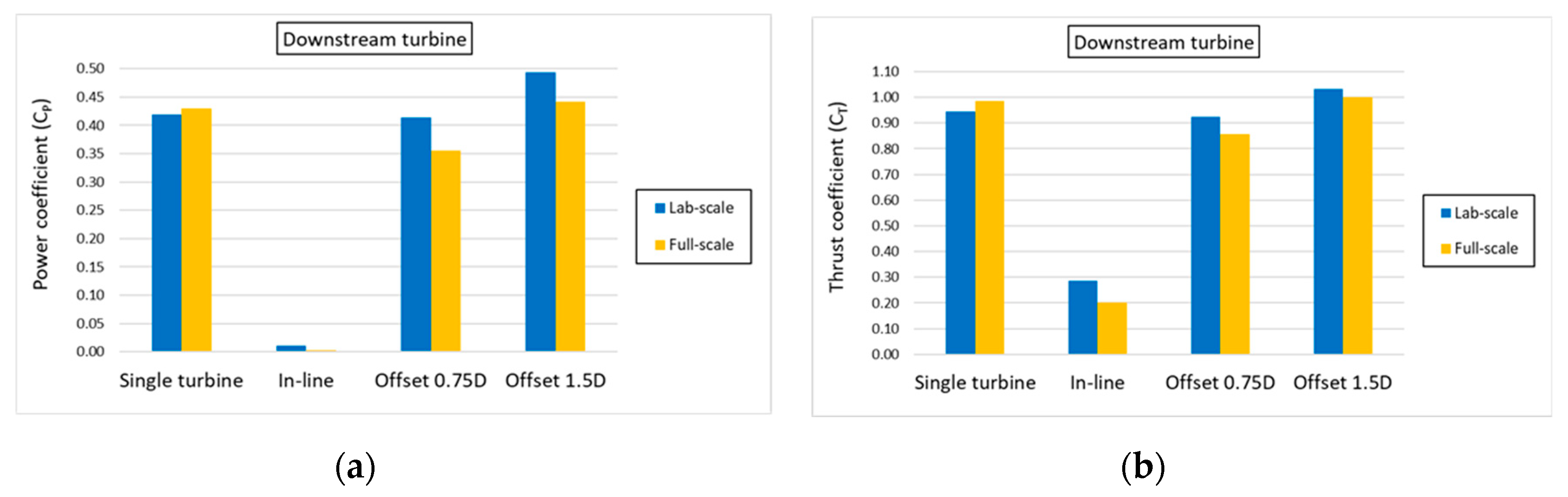
Figure 11 shows a comparison between real-scale and laboratory-scale results, in terms of
CP and
CT of the downstream turbine, in the absence of waves. For the sake of brevity, only the results relating to power are discussed, since as already seen, the thrust is affected in a similar but reduced way. The in-line configuration, which had already proved unfavorable, undergoes a further reduction in power. The influence of blockage is greater in cases with offset, where there was a greater proximity of the turbines to the side walls of the laboratory. In the case with an offset of 0.75
D, the downstream turbine previously worked in a similar way to an isolated turbine, with a power only 1.3% lower, while now it is 15.2% lower, showing that in reality, it is significantly influenced by the absence of the current acceleration that in the laboratory case was caused by the wall blockage.
Regarding the case with 1.5D offset, in the non-confined simulations, the downstream turbine performs still better than the base case, but in a decidedly lesser way since now, it only gains from the upstream turbine blockage; in fact, the increase is 5.5% against the 17.8% recorded at the IFREMER channel.
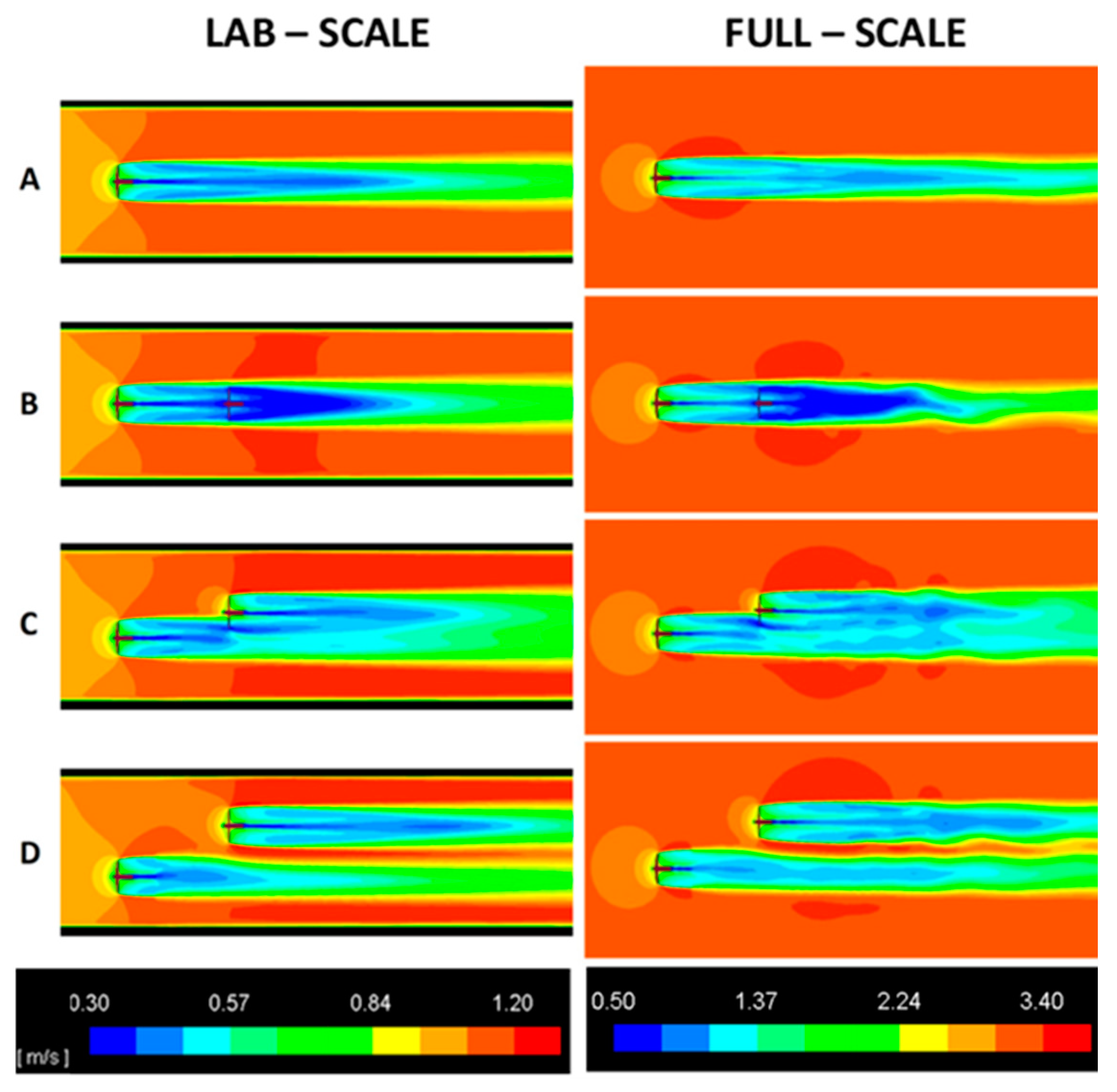
The blockage effect is more clearly visible from the comparison between the streamwise velocity fields, which are depicted in
Figure 12 on a horizontal plane. In laboratory conditions, the flow is unable to expand due to the presence of the side walls, resulting in considerable acceleration, while in unconfined conditions, there is no longer any constraint, and therefore, the flow lines are free to expand. The presence of the turbine now causes an acceleration on the surrounding flow limited to a reduced area, which does not affect the rest of the domain. It can be seen that in the cases with offset, in the laboratory-scale simulations, the proximity to the walls has an effect on a higher velocity of the flow that affects the downstream turbine and therefore there is an overestimation of the power and thrust generated by it. It can be also observed that now, the wake of the downstream turbine, with respect to laboratory tests, takes on an undulatory nature, which is explained by the fact that the field of motion free to expand around a globally stocky object generates a Von Karman-like undulating wake [
34]. In conclusion, the motion field is more realistically represented by unconfined simulations, while it is distorted in simulations in narrow experimental channels.
4.2. Effects of Turbine Offset under Current-and-Wave Conditions in Case of Full Scale
Passing from the laboratory scale to the full scale, some of the wave characteristic parameters are kept constant (Ursell number, steepness, depth/length ratio), whereas the wave height and length are scaled by a factor of 20, as it was done for the turbine diameter and the water depth, resulting in 3 m and 112 m, respectively. Since the wave period depends on Froude scaling, it would result respectively in 6.39 s or 6.97 s by setting
Fr = 0.22 (as achieved with a current speed of 4.47 m/s, for a perfect similarity) or
Fr = 0.15 (coherently with a current speed of 3 m/s). As mentioned previously, a current velocity of 3 m/s together with waves of a period of about 7 s would be more representative of realistic tidal sites [
40,
41].
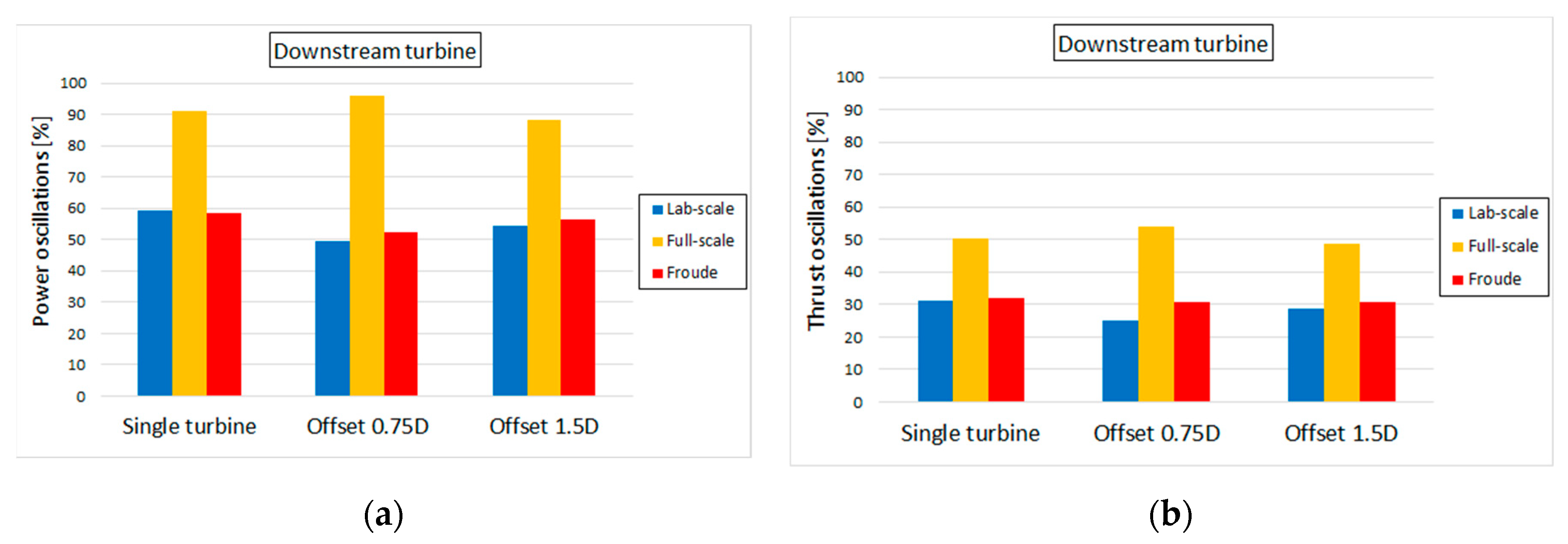
With the aim of verifying how much the results change if the condition of perfect similarity is lost, in this section, the predictions obtained by simulating both Froude numbers, and therefore both the current speed–wave period pairs, are shown and discussed. In
Figure 13, the results concerning the Froude numbers of 0.22 and 0.15 are respectively depicted in red and yellow for cases A, C, and D (case B is not reported because of the exaggerated values of fluctuations).
When the similarity with the laboratory scale is maintained, it can be observed that blockage does not appreciably affect the power and thrust fluctuations of the single turbine. However, some relatively small effects are visible in case of offset for the downstream turbines; in fact, the fluctuations appear slightly higher in the unconfined environment. This can be justified considering that in the real environment, the lateral flow accelerations are prevented, and therefore, the velocities generated by the waves play a more important role in determining the instantaneous value of flow the axial velocity.
If the similarity with the laboratory scale is lost, the results appear very different, suggesting an untrue and exaggerated effect of the blockage. As can be seen, in this case, the oscillations induced by waves in thrust and especially in power increase significantly from small scale to real scale. Yet, the increase is due to the wave longer period and to the lower current speed adopted compared to a perfect similarity to Froude, which has repercussions in a greater penetration of the waves in depth and greater changes in the flow velocity [
42]. It has to be underlined that this effect is false; in other words, it only depends on the inconsistent choice in the setting of the
Fr (0.15 instead of 0.22).
5. Conclusions
A Virtual Blade Model has been adopted to study the performance and wake of a horizontal axis tidal stream turbine under current-only and wave and current interactions. The model has shown to predict accurately the operation of a small-scale turbine, and it allowed further analysis of interacting turbines at a small scale and at a full-scale operating in unconfined environments given the savings in calculation times arising with the implementation of the Virtual Blade Model.
The interaction of turbines was investigated using two case scenarios: in-line (back to back turbines) and with an offset of 0.75D and 1.5D between the upstream and downstream turbine measured from the turbine hub center. In-line turbine configurations were used to show the influence of the upstream turbine to the downstream device. In the analyzed conditions, the turbine has power loses over 80% if aligned, while it seems to gain 4% with a 0.75D offset and as much as 17% with a 1.5D offset.
Furthermore, it has been shown that the blockage effect caused by the confinement of laboratories can significantly influence the performance results of the turbine. In fact, the CP and CT values of the downstream turbines are visibly different, especially in the cases with lateral offset, in which in laboratory conditions, the devices were close to the walls of the tank. For current-only conditions and in the case with an offset of 0.75D, the performance of the downstream turbine is significantly lower than the base case (about 15% instead of 1%). For the offset case of 1.5D, even in unconfined full-scale conditions, the downstream turbine still performs better than when it is alone, but in a lesser way, only with an increase of 5%.
Repeating the simulations in the presence of waves in unconfined real conditions, it is revealed that a correct choice of Froude number aimed at maintaining the complete similarity in scaling-up problems is essential to prevent mistakes in the interpretation of the results of the simulations and in particular in the evaluation of the wall blockage effects. In fact, when the similarity is maintained, the blockage only entails a small underestimation of the power and thrust fluctuations for the downstream turbines, proving that also narrow tanks or flumes are reliable methods to check the effects of waves on small-scale turbines. On the opposite, if the similarity is not respected, the predictions are not dependable, since the role of blockage could be erroneously amplified.
To conclude, the BEM-CFD model based on the VBM User-Defined Function has proven to be a useful tool to be used together the experimental tests. In particular, it can be adopted both to support the planning of an experimental matrix and to predict and correct the blockage effects in phase of up-scaling to the real dimensions and operating conditions.
A future development could be the reproduction of even more realistic marine conditions with high background turbulence. During the work done by [
34], it was verified that greater environmental turbulence profoundly affects the length and strength of the wake produced by a marine turbine, and it would be interesting to evaluate how this affects the interaction between two coupled turbines.


