Article

Arctic Vision: Using Neural Networks for Ice Object Classification, and Controlling How They Fail

Department of Marine Technology, NTNU Norwegian University of Science and Technology, 7491 Trondheim, Norway
*
Author to whom correspondence should be addressed.
J. Mar. Sci. Eng. 2020, 8(10), 770; https://doi.org/10.3390/jmse8100770
Submission received: 3 September 2020 / Revised: 25 September 2020 / Accepted: 28 September 2020 / Published: 30 September 2020
(This article belongs to the Special Issue Human-Automation Integration in the Maritime Sector)

Abstract

:
Convolutional neural networks (CNNs) have been shown to be excellent at performing image analysis tasks in recent years. Even so, ice object classification using close-range optical images is an area where their use has barely been touched upon, and how well CNNs perform this classification task is still an open question, especially in the challenging visual conditions often found in the High Arctic. The present study explores the use of CNNs for such ice object classification, including analysis of how visual distortion of optical images impacts their performance and comparisons to human experts and novices. To account for the model’s tendency to predict the presence of very few classes for any given image, the use of a loss-weighting scheme pushing a model towards predicting a higher number of classes is proposed. The results of this study show that on clean images, given the class definitions and labeling scheme used, the networks perform better than some humans. At least for some classes of ice objects, the results indicate that the network learned meaningful features. However, the results also indicate that humans are much better at adapting to new visual conditions than neural networks.

Graphical Abstract

1. Introduction

Computer vision using convolutional neural networks (CNNs) has revolutionized automated image recognition and object detection in recent years. It is by far the most successful technique for image classification and segmentation to date and is used in applications ranging from autonomous vehicles [1,2,3] to the detection of cancer cells [4,5]. With increasing traffic in the Arctic due to the melting of the polar ice, it would be desirable to exploit this powerful technique for navigational assistance to captains, potentially reducing the risk of collisions and damage.
However, the Arctic poses different challenges for a machine learning system than other common use cases, such as autonomous driving or recognizing objects in well-lit rooms. First, labeled data are still relatively scarce. Although more and more near-field image data are becoming available from the region, the labeling of such data is extremely costly. The WMO [6] defines 220 different classes of ice objects, many of which are overlapping or difficult to distinguish. For example, the difference between a floeberg and a floebit is size, which is difficult to identify with accuracy in an image. Even if one uses a very small subset of these classes (such as the nine used in this work), the labeling needs to be done by experts, simply because most people are unable to distinguish between classes. Furthermore, the labels have a degree of subjectivity to them, as the viewer’s interpretation of the image (relating to, e.g., the scale and color balance of the ice objects) impacts the labels. This is in contrast to the labeling of images used, for example, in autonomous driving or more general object detection, wherein most people are familiar with the domain, the task of labeling can easily be crowdsourced, and the labels are largely objective.
Another important difficulty with computer vision in the Arctic is that visual conditions vary greatly. This has two main implications: First, the assumption that training and testing data are independent, identically distributed (i.i.d.), which is typically made for supervised machine learning, does not hold unless one can get enough samples of all the variations of weather and visibility conditions. This is an unrealistic demand, as there is no way to control the weather, meaning data collection would be extremely time-consuming. Second, it has been shown that neural networks do not handle distorted images well [7,8]. The poor visual conditions in the Arctic can be seen as a form of noise, so it is unlikely that CNNs trained in the normal manner will be robust to such conditions. Finally, the fact that snow and ice are highly reflective, meaning some features can be reflected in each other, is also likely to make the classification of such images more difficult.
In the present work, an analysis of how CNNs fare when used for classifying ice objects on close-range optical images of ice cover is presented. It includes the use of several forms of semi-realistic image distortions to simulate the difficult visual conditions of the Arctic, caused by natural phenomena such as fog, low light, and snow, as well as a comparison of the performance of a computer model with the performances of human experts and novices. Furthermore, to counteract the tendency of the model to be biased towards predicting the absence of ice objects even when they are present in the image, a loss weighting scheme is proposed and analyzed. We argue that avoiding such biases is important for the use of automatic ice recognition, to avoid missing potentially dangerous objects.

1.1. Related Work

1.1.1. Training CNNs With Imbalanced Data

It is well-known that a neural network is dependent on a good training set to learn a meaningful function. However, when the training set is imbalanced, meaning some classes are much more common than others, the network will typically tend to predict the majority classes too often, and never or very seldom predict the minority classes. This behavior is undesired, as it could be very important for the network to detect rare classes (for example, even though brash ice is more common than icebergs, it is much more important to avoid icebergs when navigating). For this reason, multiple methods of dealing with such class imbalances have been proposed, an overview of which can be found in [9].
In general, one can differentiate between two classes of methods for handling class imbalance. The first is data resampling, which works by adding or removing samples from the dataset to balance it. In its simplest form, one can oversample [10,11,12] or undersample [10] the dataset by copying or removing images from it. A more sophisticated method for data resampling is the SMOTE algorithm [13], which synthesizes new samples of minority classes automatically. In the other class, the methods involve modifying the network or loss function. A common way to achieve this is through some sort of weighted loss [14,15,16], where the importance of different classes can be weighted against each other. This weight can be based only on the class of the sample [14], or on the class and prediction [16].
In many cases, these two approaches are interchangeable. Indeed, in the absence of random augmentation of images, oversampling and weighting samples with a given class can yield the same result. However, there are some intricacies connected to both. First, when using random augmentations of images before using them for training, oversampling introduces new images to the network (as the image is sampled more often), possibly enlarging the known input domain by a small margin. Loss weights, on the other hand, can be more flexible than resampling, as they can be dependent not only on information known a priori but also on the results of the training up to that point. Finally, the use of SMOTE or similar techniques actually introduces completely new samples to the training. However, the generation of such samples is not trivial when the input domain is large (e.g., when using images); therefore, these techniques are often not applicable.

1.1.2. Comparisons of Humans and CNNs

Several studies have looked at how well CNNs compare to humans on the task of image classification with distorted images. In [7], the authors found that neural networks are unable to generalize to kinds of distortions not seen during training, while humans are relatively robust to such changes. Indeed, even when including some kinds of distortions in the training set, it did not make the models robust to any other noise than the type included.
Similarly to reference [7], Dodge and Karam [8] found that humans are much more robust to distortions in images than computers. Their results show that even when including some examples of a given distortion in the training set, the CNN performed worse than the human participants.
The two previously mentioned works used relatively similar testing procedures, with images of well-known objects and settings that made the conditions for the human participants as similar to those of the computers as possible (e.g., by limiting the time the participants saw the images), thereby making them fair comparisons.

1.1.3. CNNs for Close-Range Ice Object Detection

In [17], a novel CNN architecture for semantic segmentation of river ice in images from an unmanned aerial vehicle (UAV) was developed. The network consists of two channels, one deep for extracting multi-scale semantic features, and one shallow for capturing small-scale targets. Their results show that the model successfully outperforms the state-of-the-art on their task. For a similar task, Ref. [18] trained several state-of-the-art networks using very limited data. They showed that even with very little data available, the CNN models outperformed a support vector machine (SVM) trained on the same data. Both of these works are relevant to the present work, but not directly applicable, as ice floating in the ocean looks different to and has other properties than that floating in rivers. Furthermore, an image captured from a UAV will often look different than one taken from onboard a vessel, especially with regard to shadows, and a UAV might not always be available in the High Arctic due to the harsh environment.
Kim et al. [12] present the initial results of using CNNs to recognize ice objects floating in the sea from near-field imaging, showing that a neural network can learn to recognize some forms of ice. They present an analysis of the effect of network architecture, and some initial results of the effects of simple distortions of images. Kim et al. [19] also performed image segmentation on ice images. Their results were promising, but not perfect, which they attributed to the small amount of available training data.
Although there is relatively little published work for this specific task, a lot of work has gone into the analysis of ice objects in synthetic aperture radar (SAR) images or using other techniques. For example, Ref. [20] identified ice floes in satellite images using mathematical morphology and clustering, and [21,22] used pulse coupled neural networks. Other researchers [23,24,25] used a gradient vector field snake algorithm to analyze ice floe distributions or parameters. Finally, Ref. [26] used a combination of image processing and analysis methods to find several parameters of the ice cover, including partial ice type concentration and floe size.
The present work investigates the use of CNNs for floating ice object classification in close range images, similarly to [12]. However, a more in-depth analysis of how the networks perform, especially in the presence of visual distortions, is given, to provide insights for further development of the technique. Furthermore, a comparison to human experts and novices is given, providing a benchmark for how well the networks perform. The experiments with the human participants differentiate themselves from the previous works [7,8] in that the experiments reported here measured how humans performed given their best chances. Specifically, the study did not utilize a time limit, allowing the participants to inspect the images for as long as they wanted. The results of the work are an important step towards creating systems for automatic data collection, along with navigational aid, for the increasing traffic in the Arctic.

2. Materials and Methods
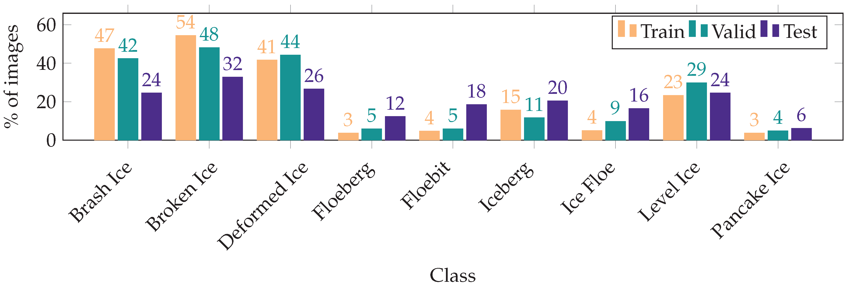
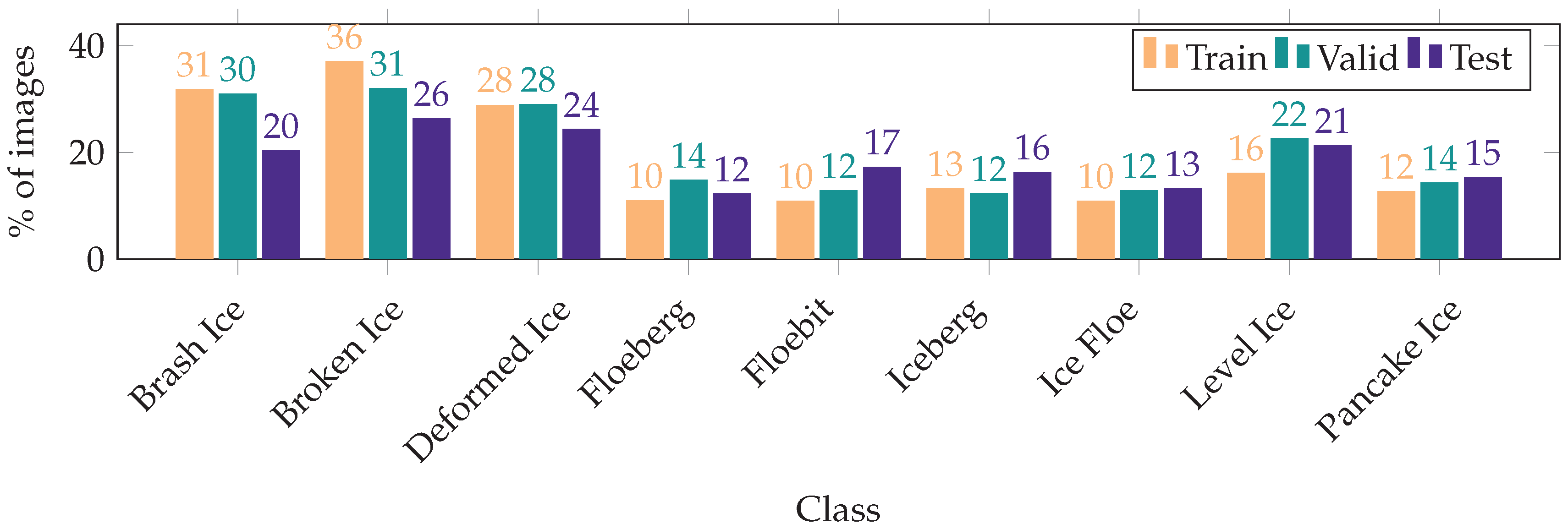
2.1. Dataset

The dataset used in this work consists of 738 images containing ice objects. Most are taken in the Arctic zone, although there are some examples from Antarctica as well. Of the images, 689 were used for training and validation, while 49 were used for testing. The training data were further split into training and validation sets: 85% for training. All splits were done randomly; however, to be able to compare the effect of different parameters, the splits were only calculated once, and reused for all experiments. Most images were taken from onboard vessels, either from mounted cameras, or manually, typically (but not exclusively) from the bridge. There is a variety of image qualities and kinds of ice objects. Most images were taken in good weather conditions with good visibility, although there are exceptions to this. The images have been acquired from various sources, including Google and Yandex images, publicly available image streams from vessels, and private pictures. The choice of having a large variance in the images, e.g., regarding camera placement and image quality, was made both to make the model able to analyze a larger variety of images, and due to relatively little available data.
Before training, each image was classified as containing any number of the nine ice object classes defined in Table 1. However, as can be seen in Figure 1, there is a huge class imbalance, in that a very large portion of images belong to one of the classes brash ice, broken ice, or deformed ice. This is likely due to several factors: First, some types of ice objects are simply more common than others. For example, pancake ice is relatively rare, while brash ice and broken ice are common, especially in the marginal ice zone and areas where ships travel. Second, some forms of ice objects, such as deformed ice and icebergs, can be more interesting subjects in a photograph than, e.g., level ice, so tourists in the Arctic or Antarctic are more likely to capture images of them. Regarding tourists, it is also important to remember that very young ice, such as pancake ice, is typically formed during early winter, when there is little light and there are few tourists, further increasing the data imbalance.
Training a neural network with imbalanced data will make it biased towards the majority classes. When the imbalance is as bad as here, the network could be expected to never or very seldom predict, e.g., pancake ice for a new image. This is undesirable, as the imbalance could as well be an artifact of the dataset as of the natural world, and we would like for the network to base its prediction on the image content rather than a (possibly incorrect) statistical distribution of the existence of ice objects. For this reason, oversampling was performed, meaning images with minority classes were duplicated in the datasets. Note that oversampling was done after the data splits, to avoid duplicate images in different sets. This led to the class distributions shown in Figure 2. Although still not perfectly balanced, it was much closer than before, which should help the network avoid making predictions solely based on a statistical distribution.
During training, random image augmentations were performed on the images. Specifically, random flipping along the x-axis, rotation, zoom, brightness, contrast, hue, and saturation adjustment were performed every time an image was used for training. This enlarged the input domain known to the network and meant the effect of oversampling was not simply showing the exact same image to the network multiple times, but instead introducing new, somewhat different, images. Note that this data augmentation is not the same as the distortions mentioned later in this section and the rest of the paper. Those distortions were applied during testing to measure the robustness of the network, as opposed to during training.

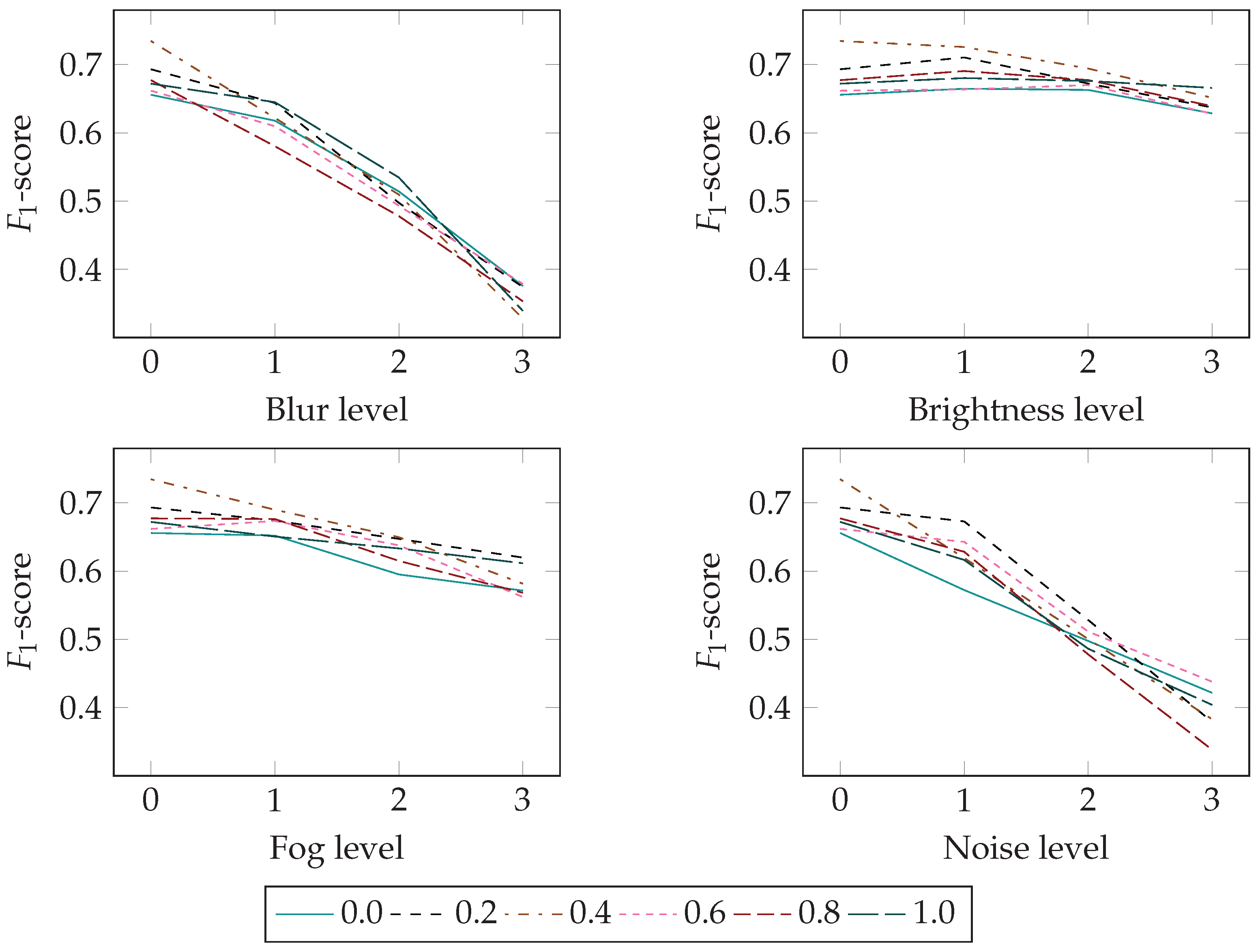
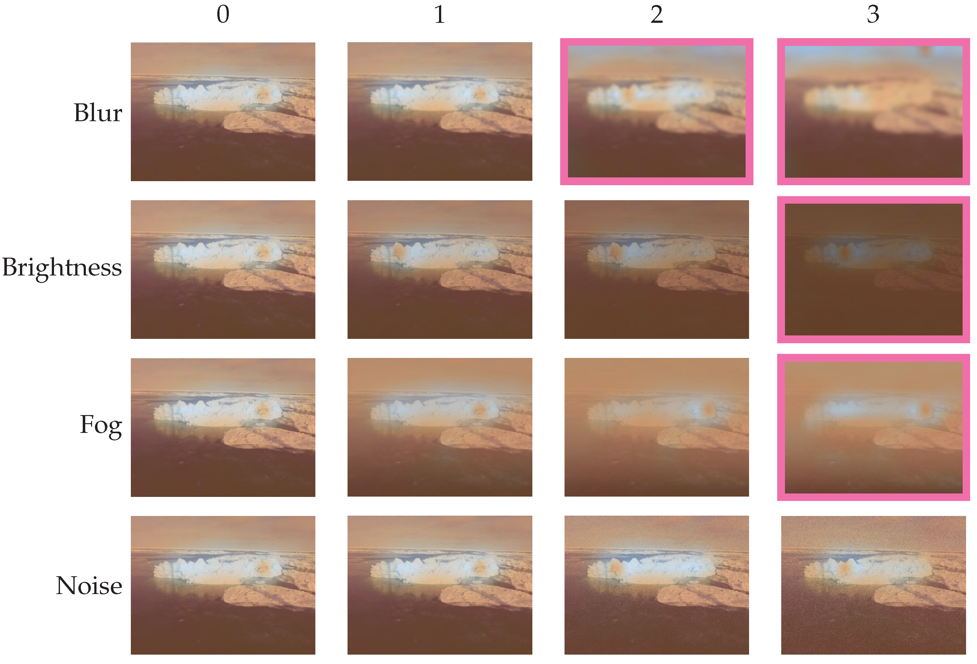
2.2. Image Distortions

The visual conditions in the Arctic are often of variable quality, with snow, fog, darkness, and other elements of the area impacting them. To test the robustness of neural networks to such conditions, we employed four semi-realistic image distortions:
  • Image blur, which can happen due to snow, rain, or water on the camera lens.
  • Brightness decrease, which imitates the visual conditions at night.
  • Synthetic fog.
  • Gaussian noise, which is similar to the effect of using a high ISO on the camera.
Each distortion was applied at three different levels, and an example of their effect is shown in Figure 3. These distortions were only used during testing, so the networks were not subjected to them during training (as opposed to the random augmentations mentioned in the previous section, which were used to diversify the training set).

2.3. True Negative Weighted Loss

The data in this work are sparse, meaning most images only contain one or a few of the nine possible classes. During initial trials, it was observed that this led the network to be biased towards predicting very few classes in an image, even after the data oversampling. To discourage this behavior, we propose an adaption of the loss function used for training.
The goal of this modified loss is to avoid a model that predicts the absence of all or almost all classes for many images. This is achieved by introducing a loss weighting scheme, as discussed in Section 1.1.1, weighting the loss values for samples and classes where both the label and predicted label is 0 (meaning not present in the image) by a weight λ t n , 0 < λ t n 1 . Such a prediction is called a true negative prediction, and we call the modified loss the true negative Weighted Loss, L t n . Its definition is shown in Equation (1).
L t n ( x , y c ; θ ) = λ t n L o ( x , y c ; θ ) , f p r e d , c ( x ; θ ) = y c = 0 L o ( x , y c ; θ ) , otherwise .
In the definition, L t n is the modified loss, x—the model input, y c —the class label for input x and class c, L o —the original loss function, λ t n —the true negative weight, θ —the network parameters, and f p r e d —a function to get the prediction from a network (where f p r e d , c is the prediction for class c). Note that it is not necessary that f p r e d = f , where f is the neural network. Indeed, this is rarely the case, and a typical definition of f p r e d , which is used in this work, is shown in Equation (2),
f p r e d ( x ; θ ) = 1 , σ f x ; θ > 0.5 0 , otherwise ,
where σ is the sigmoid function. By varying λ t n , it is possible to control the balance between making correct true negative predictions more certain at the cost of more likely predicting the absence of classes actually in the image (called a false negative prediction), and avoiding a bias towards only making negative predictions.
It is important to note that even in the extreme case where λ t n = 0 , this loss does not remove all encouragement for the network to correctly predict the absence of any class in an image. The reason for this is that the weights are still modified for the image as long as it is misclassified, thereby pushing the model towards predicting the absence of the class in the image. However, this method simply avoids the model continuing to make such predictions more and more certain, which would typically happen at the cost of failing to recognize the class when it is present in an image.

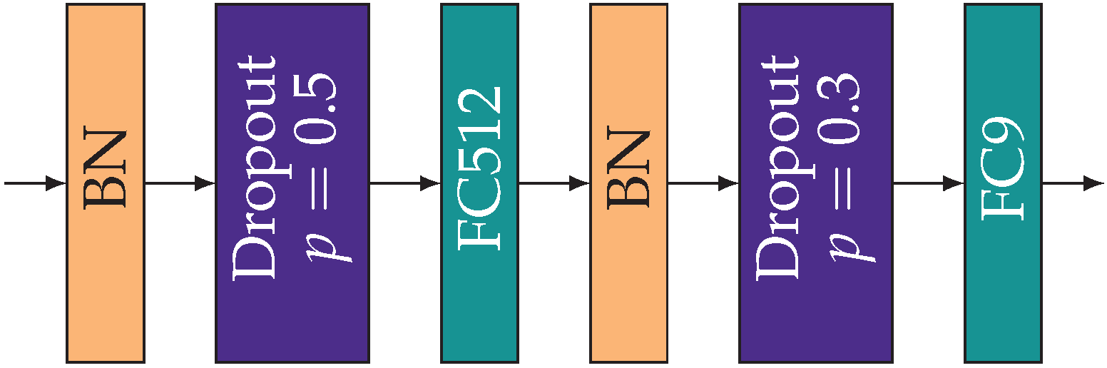
2.4. Training Procedure

For all experiments in this work, a pre-trained ResNet34 [27] was used. It was pre-trained on ImageNet [28] and is freely available from the torchvision model zoo [29]. For retraining the networks, the 1-cycle training scheme from [30] was utilized. We used the Adam optimizer [31] with decoupled weight regularization [32]. Images were randomly augmented as described in Section 2.1 and normalized to the mean μ and standard deviation σ in Equation (3), as per the torchvision documentation.
μ = 0.485 0.456 0.406 , σ = 0.229 0.224 0.225
Before training began, the last fully connected layer in the network was exchanged for the block shown in Figure 4. Training then consisted of two phases: For the majority of the training, the original network was frozen and only the new layers were updated. Following that, all layers were unfrozen and training continued. During this last stage, the learning rate varied per layer, with the learning rate α i for layer i from the beginning of the network given by Equation (4). Here, layer 0 is the first and layer N is the final layer. Table 2 shows the training parameters used in this work. All networks used those parameters. Two models were trained for each value of the true negative weight, with all other hyperparameters being the same. The average metrics of the two are reported in the results, to avoid overly positive or negative results due to a good or bad initialization of the network parameters.
α i = α 0 α N α 0 N i , i = 1 , , N

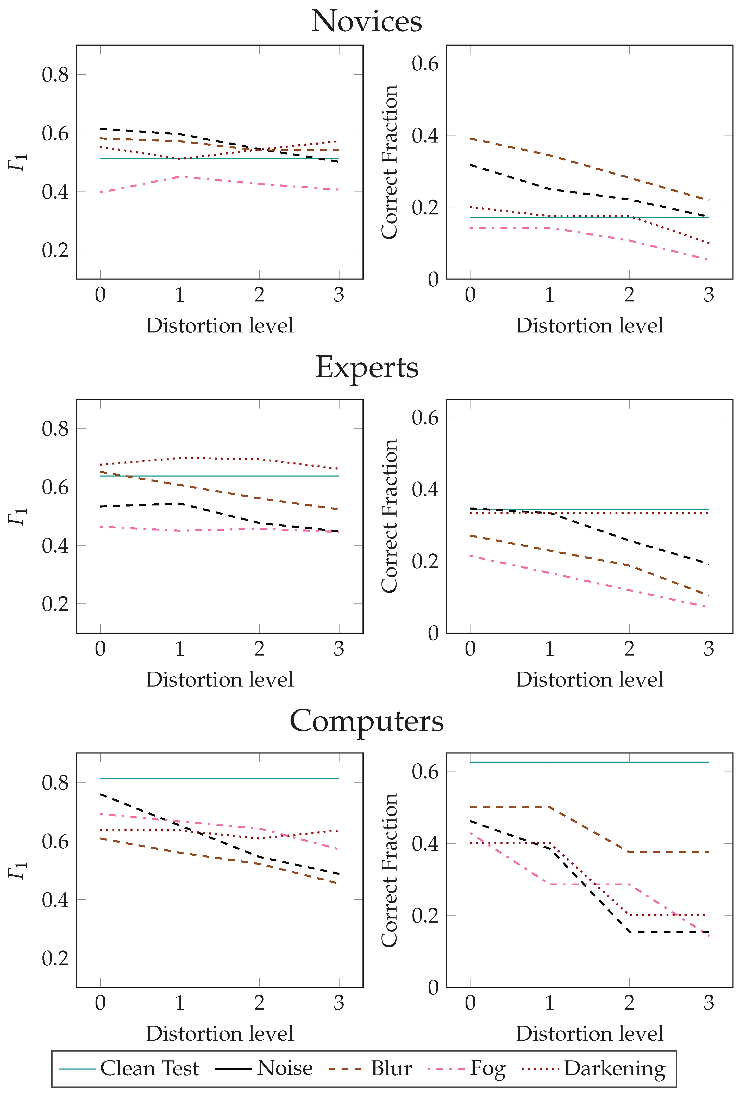
2.5. Human Experiments

The results of the network classifications are compared with the results of the human classification experiment described in [35]. A recap of the methodology used is given here. In the experiment, two participant groups were used, one consisting of eight novices with no prior experience with ice object identification, and one consisting of six experts in the field. Initially, the participants were shown a set of images with their respective classes as a training phase, before starting the classification test. During the test, the participants were first asked to classify a set of non-distorted images. The results of this initial test form a baseline for the human results. After the clean test phase finished, the participant was shown distorted images and asked to classify them. Each image was first shown at its maximum level of distortion. If a participant successfully classified the image (meaning selecting all correct and no incorrect classes) at a given level, that image was recorded as successfully classified at all lower distortion levels as well (similar to the procedure in [8]). If the image was not successfully classified, it was later shown at a lower distortion level. This continued until the participant either classified the image correctly or failed to classify it with no distortion applied. The participants had no time limit when classifying the images, and no cap on how many classes they could select. To keep the task for the humans similar to that of the neural networks, the participants were not told about the distortions beforehand. Once they had submitted their classification for a given image, they were not able to change it.

3. Results

Multiple performance-metrics were used to evaluate the networks in this work. Specifically, we employed the accuracy ( a c c ), balanced accuracy ( a c c b ), geometric mean ( μ g ), precision, recall, and F 1 score. The accuracy is the fraction of correct classifications (both of the presence and absence of classes) divided by the total number of classifications. For problems with many classes compared to the number of classes present in each image, the accuracy tends to be artificially high (as it becomes easy to predict the absence of a class correctly), so the balanced accuracy and geometric mean are often used as better metrics of how well the network really performs. Precision denotes how large a fraction of predicted classes is actually in an image, while recall denotes the fraction of classes in the images the network manages to predict. The F 1 score is a balance of precision and recall with the two given equal weight. The definitions of the metrics are shown in Table 3.
Figure 5 shows how the test metrics vary with the true negative weight, λ t n . The metrics shown are the averages of the metrics for the two models trained for each value of λ t n and were calculated on the oversampled test set. The error bars show the minima and maxima of the two models. As the trends of all the metrics are relatively similar, the rest of this paper uses the F 1 score unless otherwise noted, to make the discussion easier to follow.
A more detailed view of how the networks perform for the different ice object classes is shown in the heatmap in Figure 6. Again, the values are the averages of two networks and were calculated over the oversampled test set. The figure shows that the network performance varies across the different classes, with ice floes having an average F 1 score of 0.22, while floebergs have an average score of 0.84.
When looking at the effect of distortions, Figure 7 shows that all distortions negatively affect the models, with blur and noise impacting the models the most. On average, blur and noise degrade the F 1 score by 0.33 and 0.29, respectively, from clean to most distorted images, while brightness and fog degrade it by 0.04 and 0.10. The metrics are the means of two models trained with each value of λ t n , calculated on the oversampled test set.
From the results in Figure 5, it is clear that one of the models with true negative weight λ t n = 0.4 performed the best when analyzing clean images, while for distorted images none of the models performed notably better than the rest. For this reason, that model was used for comparison with the human participants and the in-depth analysis in the discussion.
Figure 8 shows how the performances of human experts and novices compare to the model. Table 4 shows how much each group is affected by the distortions. The data indicates that, given the labeling scheme used in this work, the CNN performs better than both groups of humans on clean images. However, this form of experiment can put the experts at a disadvantage, which is discussed more in Section 4.4. Furthermore, it is clear from the table that humans are more robust to the distortions, with their average degradation being at the same level or better than the minimum degradation for the computer. As was expected, the data show that the experts perform better than novices.

4. Discussion

Based on the results of the last section, a few relevant questions come to mind: What is the effect of applying the true negative weighted loss to the model during training? What do the models see in the images that creates such a gap between their performances on some classes, and how do the distortions affect this? Finally, can we glean any insights into the differences between how humans and computers classify ice images? The rest of this section will address those questions.

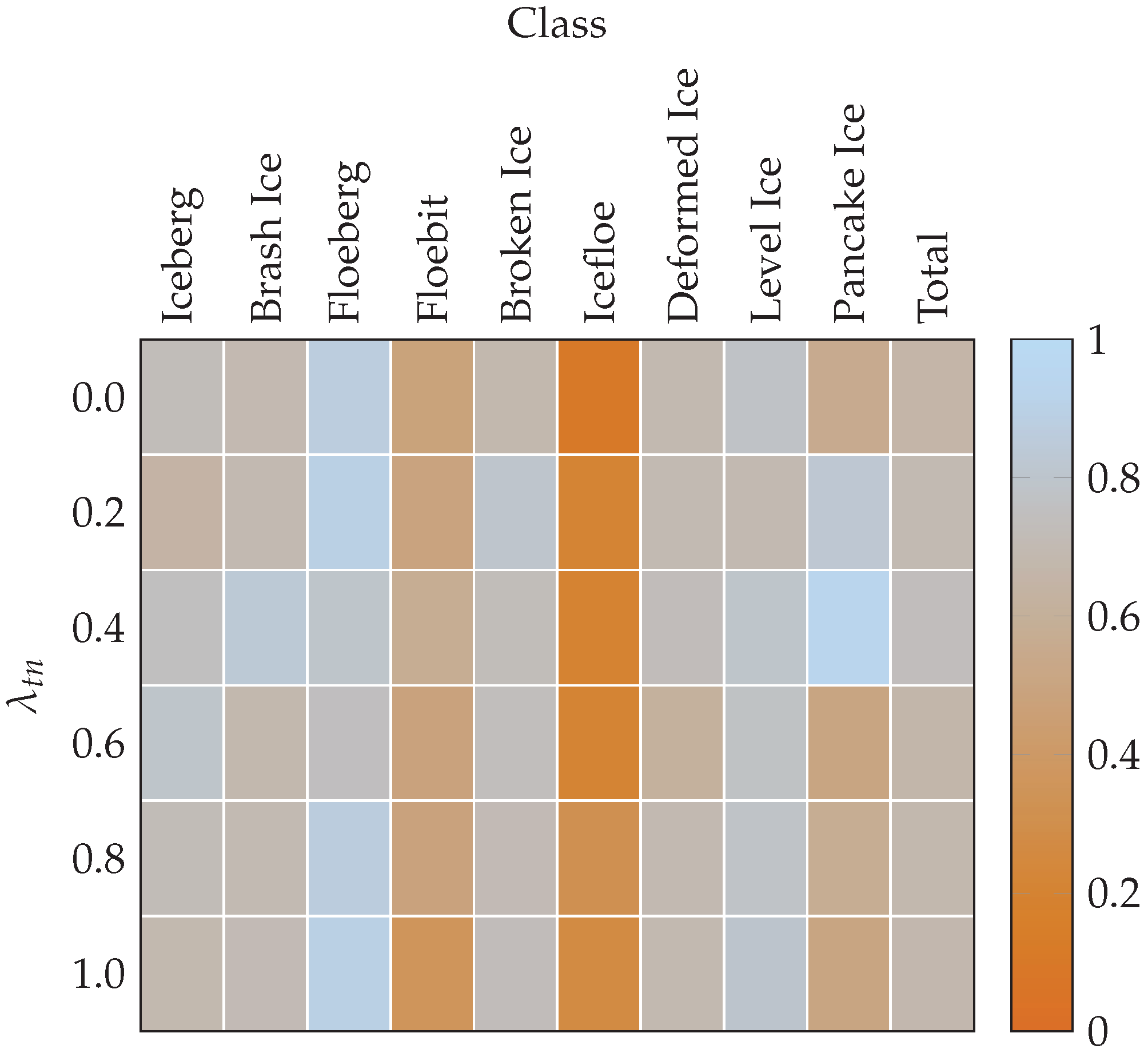
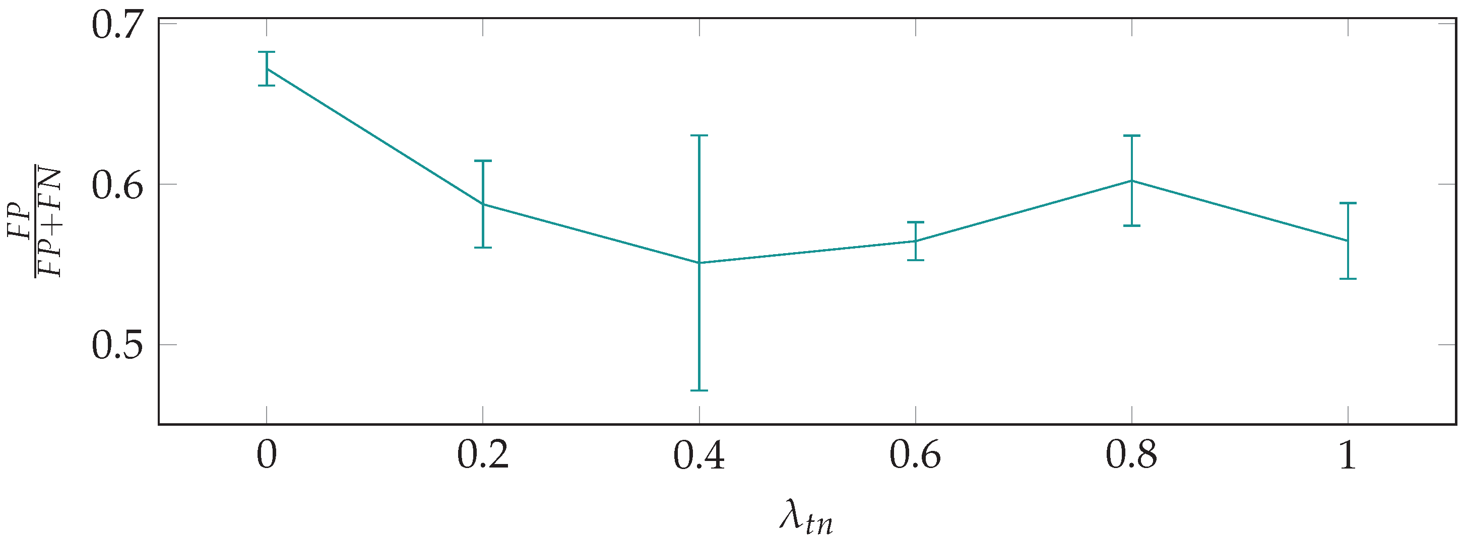
4.1. Effect of the True Negative Weighted Loss

Varying λ t n , the true negative weight, in the training loss, has little effect on the test-metrics of the networks. This can be seen in Figure 5. The figure shows a slight increase for λ t n = 0.4 , but it is uncertain if this is an indication of that value being superior or if it is an artifact of the specific training run or random initialization of network weights. This hypothesis is further reinforced from the fact that Figure 9 shows a very large variance for the models with λ t n = 0.4 compared to the rest, indicating that these two models, trained with the exact same hyperparameters, behave very different to each other.
What varying λ t n does change, however, is the distribution of false predictions. Figure 9 shows the portion of false predictions being false positives for varying values of λ t n , and it is clear from the plot that lower values of λ t n tend to lead to a higher fraction of false positives.
Therefore, based on the previous observations, it is possible to change the behavior of the network when it fails, largely without affecting its ability to correctly recognize other elements of an image. This gives some general insights into the flexibility of neural networks: Although one is unable to increase the number of correct classifications (using this specific method), one can still make the network’s behavior fit better to a use case. For ice object recognition, it is reasonable to assume one would prefer a system warning about some dangerous ice object a bit too often over a system that allows you to miss one. Of course, this is not necessarily true for all ice classes; e.g., it is likely unimportant if the model misses some brash ice from time to time. However, it could be extremely important not to miss icebergs, as colliding with them could be catastrophic.

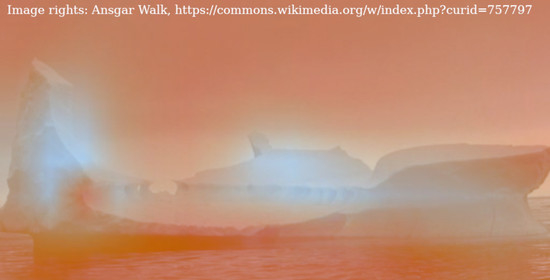
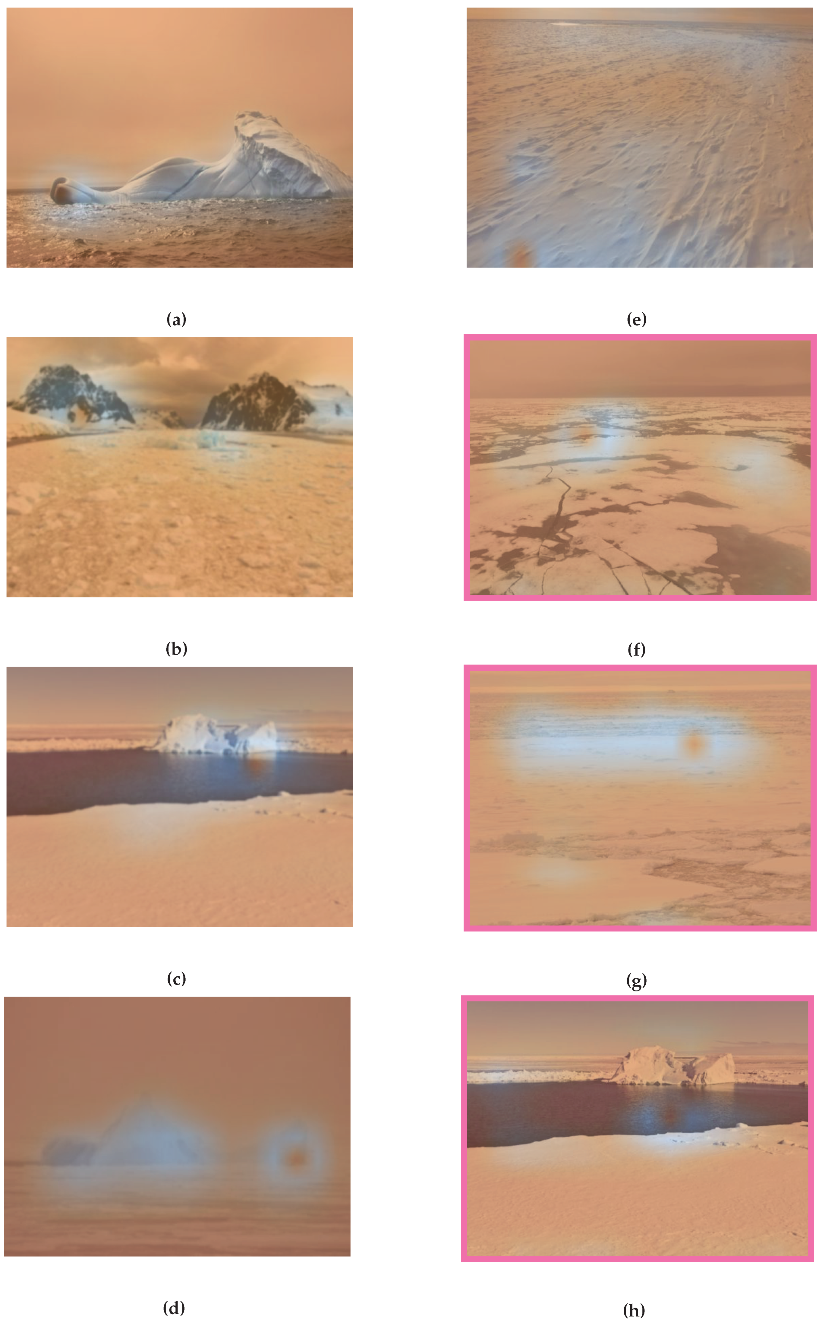
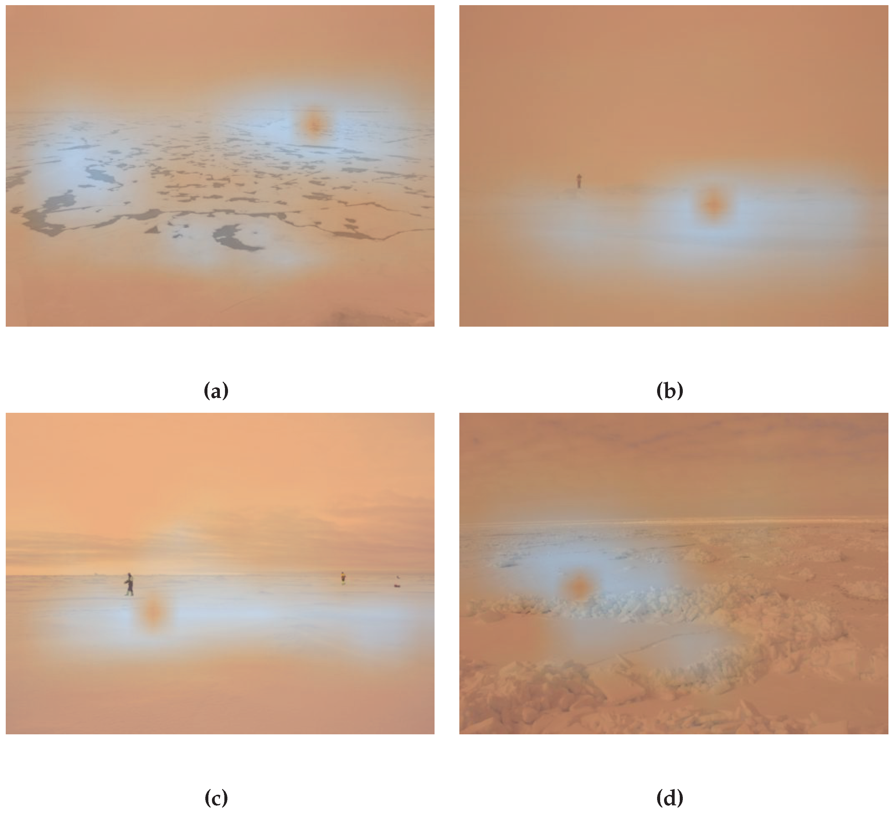
4.2. What the Network Sees

From Figure 6, we see that the network performs very well for some classes, such as icebergs, floebergs, and level ice, while failing spectacularly on others, e.g., ice floes, floebits, and to a certain degree pancake ice. To understand this difference, it is useful to investigate which areas of the image are of importance for the network to classify. A method for this is the Grad-CAM [36], which uses the gradient of classification scores with respect to the activations of a layer to find areas of interest to the network. In all Grad-CAM images in this work, the activations of the last residual block are used.
Figure 10 illustrates the difference between a class the network successfully manages to recognize and one that it does not. Figure 10a–d shows the Grad-CAM images for iceberg activations, while Figure 10e–h shows those for ice floe activations. It is clear that the network indeed looks at the icebergs for classifying them, even though the mountains in Figure 10b fool the network into believing they’re icebergs as well. It should be noted that since most of our dataset is from offshore areas in the Arctic, mountains and other shore features are not common in the dataset. Therefore, it is not surprising that the model has some problems with this image from Antarctica.
Regarding ice floe images, it is immediately apparent from the images that instead of looking at ice floes as a whole, the network only focuses on some few parts, typically around the edges of the floes, or, in cases where there are few or no edges, seemingly random locations. Now, an ice floe is not defined by its boundary, so there is a clear discrepancy between what the network has learned and the real world.
Based on our study, it is currently challenging to understand what makes ice floes more difficult to recognize than other ice objects. One guess is that the network has a problem recognizing ice features that are not located around a small area of an image, as an ice floe has few defining characteristics on a local scale. If this is true, it would be reasonable to assume the class level ice will exhibit similar behavior. From Figure 6, it seems that the network is actually very successful at classifying level ice. Even so, the Grad-CAM images for level ice activations in Figure 11 show a more nuanced view. Indeed the images show the same trend towards looking at specific parts of the ice, instead of the ice as a whole. The difference between the two classes seems to be that the network finds a useful descriptor for level ice in local areas, which makes sense because the idea of “levelness” can be applied to patches of varying sizes.
There are a few other plausible reasons for the difficulty with ice floes. One is that nothing in the training set explicitly teaches the network about open water, which often surrounds ice floes in the images. This could lead to models not understanding that the floe is not surrounded by ice, and making the distinction between ice floes, and e.g., level ice less apparent. Furthermore, the leading descriptor for an ice floe is its size, and since the dataset contains no scale information, this is likely hard to determine for the models. Finally, ImageNet, which the models were pre-trained on, contains some ice classes, with many misclassifications, especially for a few classes, including ice floes [12]. This can lead to the model being better suited to classify the classes with many correct samples in that dataset (such as icebergs), compared to those not present or with many incorrect samples.

4.3. The Effects of Distortions

Figure 7 shows the performances of networks with varying values of the true negative weight at different levels of distortions. It is clear from the plots that a higher level of distortion leads to lower performance, although the severity of the effect varies according to the distortion type. Brightness and fog impact the F 1 scores of the models by averages of 0.04 and 0.10, respectively, while blur and noise degrade it by 0.33 and 0.29, respectively. The results do not indicate that a certain value of the true negative weight consistently handles distortions better than the others.
Figure 12 shows Grad-CAM images of the floeberg activations of an image containing a floeberg along with broken ice, with varying levels of distortions. The image was chosen for two reasons: First, because it contains a floeberg, a class the network is largely successful in classifying. Second, because the model failed to correctly classify some distorted versions of the image, so it yields a more interesting analysis. Looking at the images, it is noteworthy that the network notices the floeberg as the important part of the image in all instances, although it also starts looking at the sky in the case of the blurred images. This means that if asked the question, “Where in the image is the floeberg?” as opposed to, “Is there a floeberg in this image?” the network would be largely successful. However, since the Grad-CAM images are normalized, they do not show how strong the signal is, which is the problem here. Indeed, looking at the activations of the network, quite a few of the images would be classified as a floeberg (along with broken ice) by lowering the point at which the model marks a prediction as true. This indicates that neural networks have a theoretical ability to see even in distorted conditions, although work is needed to exploit this ability.
One problem with the given image was that the model had a tendency to label some of the distorted versions (distorted by fog or noise) as brash ice in addition to the other classes. We hypothesize that these modifications, which add elements to the image instead of making what is there already less clear, can introduce new textures and gradients in the image. This affects the network negatively, as ImageNet-trained neural networks are biased towards texture [37]. For brash ice, such misclassifications would typically not be of much importance; however, the problem points to a serious flaw in this model, one that needs to be addressed in the future.

4.4. Difference between Novices, Experts, and Computers

As can be seen from the plots in Figure 8 and degradation values in Table 4, both humans and computers are negatively affected by distortions in the images. Although humans are affected by distortions in the images, they are much more robust to them than computers. Indeed, the distortion causing the least difficulty for the computers still led to a degradation at about the same level as the average distortion for the humans. This agrees with previous studies comparing humans and computer vision [7,8], and shows the need for more robust computer vision models. However, the distorted Grad-CAM images in Figure 12 indicate that such robustness might be possible.
It appears from the plots that computers outperform humans for clean images, especially when looking at the fraction of images that were classified exactly correct, while the F 1 score is slightly closer. However, it must be mentioned that experts can be at a disadvantage here, as they might have some pre-existing notion of what each ice class is that does not match the definitions used in this work perfectly. Such a pre-learned bias, along with a possibility of them being used to being either more or less detailed than the labeling used here, can lead to lower scores on paper, though they might perform better in a real situation. Since there is a certain amount of subjectivity in ice object classification (e.g., should one label the small pieces of brash ice typically present in between broken ice?), these scores can not be seen as an objective measure of how well the experts are recognizing the ice, but rather as a measure of how much they agree with the labeling scheme used here. Such considerations do not apply to the novices, as they have no pre-learned definitions of ice classes, so it is fair to say that the network at least outperforms the novices.
A reason for the difference between the correctly classified fraction and F 1 score can be seen from the definition of the F 1 score (see Table 3), namely, that humans classify more optimistically than the computer. In other words, humans have a larger tendency to select more classes, leading to a higher score for both true and false positives, and a symmetric decrease in true and false negatives. This hypothesis is confirmed when we see that novices on average classify each non-distorted image with 2.12 labels, and experts with 2.15, while computers use on average 1.86 labels per image. Although we can increase this number by lowering the true negative weight, this did not result in a higher F 1 score in our experiments.
Finally, it is worth noting that there is a large difference between the performance on undistorted images in the different partial test sets (i.e., the images with distortion level 0). This shows how some images likely are inherently more difficult to classify for the different groups. This was expected, especially because each subset was relatively small (to limit the time needed to perform the test for humans). What is interesting is that the relative difficulty of each different set varied between the groups. For humans, the fog-dataset was the most difficult by some margin, while the computer seemed to struggle less with it.

5. Summary and Conclusions

In this work, we have presented an in-depth analysis of the use of CNNs for the classification of ice objects in icy areas. The main contributions of the work can be summarized as:
  • A loss-weighting scheme for making the trained model more likely to predict that classes are present in an image was introduced. Results show that the scheme works as intended, by avoiding an excess of false negative classifications and the possibility of missing important ice objects in images.
  • A demonstration of how CNNs can successfully recognize some ice objects in images using meaningful filters was provided, along with a discussion of why they struggle with some classes.
  • A thorough analysis of the effect of semi-realistic image distortions on the classification task was provided. It was shown that even though the network fails to classify an image, it still recognizes the area of importance in the image for the given class.
  • Finally, a comparison of the performances of human novices, experts, and computers on the classification task was given. The results indicate that for clean images, the model outperforms human novices, although it is less clear how it compares to experts. Both human participant groups handled distortions better than the network.
These results form a basis for continued work in the area of automatic ice object recognition from near field imagery, and provide some insights into the workings of CNNs in general. They provide a point to continue working from, towards automated navigational aids and data collection on Arctic vessels. For the future, relevant areas of research to improve the results include making CNNs more robust to visual distortions, improve the accuracy of the models for specific classes (e.g., ice floes), and finding more efficient methods for large-scale data collection. Furthermore, it would be interesting to compare the models in this work with ones trained on datasets that either include scale information directly (e.g., through depth images) or have an identical camera setup for all images.

Author Contributions

Conceptualization, O.-M.P. and E.K.; methodology, O.-M.P. and E.K.; software, O.-M.P., validation, O.-M.P. and E.K.; formal analysis, O.-M.P.; investigation, O.-M.P.; resources, E.K.; data curation, E.K. and O.-M.P.; writing—original draft preparation, O.-M.P.; writing—review and editing, O.-M.P and E.K., visualization, O.-M.P.; supervision, E.K.; project administration, E.K.; funding acquisition, E.K. All authors have read and agreed to the published version of the manuscript.

Funding

This research received no external funding.

Acknowledgments

The neural network training and testing was performed on resources provided by UNINETT Sigma2—The National Infrastructure for High Performance Computing and Data Storage in Norway. We thank all human participants in our experiments. Finally, our appreciation goes to the owners of the images used in this paper: Alex Cowan, Knut Vilhelm Høyland, Lauren Farmer, Natalie Lucier, Roger Skjetne, Sergey Dolya, SF Brit, Sveinung Løset, and the SAMCoT Project.

Conflicts of Interest

The authors declare no conflict of interest.

Abbreviations

The following abbreviations are used in this manuscript:
CNNConvolutional Neural Network
i.i.d.Independent, Identically Distributed
ReLURectified Linear Unit
SARSynthetic Aperture Radar
SVMSupport Vector Machine
UAVUnmanned Aerial Vehicle

References

  1. Gao, H.; Cheng, B.; Wang, J.; Li, K.; Zhao, J.; Li, D. Object Classification Using CNN-Based Fusion of Vision and LIDAR in Autonomous Vehicle Environment. IEEE Trans. Ind. Inform. 2018, 14, 4224–4231. [Google Scholar] [CrossRef]
  2. Kim, H.; Hong, S.; Son, H.; Roska, T.; Werblin, F. High speed road boundary detection on the images for autonomous vehicle with the multi-layer CNN. In Proceedings of the 2003 International Symposium on Circuits and Systems, Bangkok, Thailand, 25–28 May 2003. [Google Scholar]
  3. Ouyang, Z.; Niu, J.; Liu, Y.; Guizani, M. Deep CNN-Based Real-Time Traffic Light Detector for Self-Driving Vehicles. IEEE Trans. Mob. Comput. 2020, 19, 300–313. [Google Scholar] [CrossRef]
  4. Gao, F.; Wu, T.; Li, J.; Zheng, B.; Ruan, L.; Shang, D.; Patel, B. SD-CNN: A shallow-deep CNN for improved breast cancer diagnosis. Comput. Med. Imaging Graph. 2018, 70, 53–62. [Google Scholar] [CrossRef] [PubMed] [Green Version]
  5. Reda, I.; Ayinde, B.O.; Elmogy, M.; Shalaby, A.; El-Melegy, M.; El-Ghar, M.A.; El-fetouh, A.A.; Ghazal, M.; El-Baz, A. A new CNN-based system for early diagnosis of prostate cancer. In Proceedings of the 2018 IEEE 15th International Symposium on Biomedical Imaging (ISBI 2018), Washington, DC, USA, 4–7 April 2018; pp. 207–210. [Google Scholar]
  6. WMO. Sea-Ice Nomenclature; WMO: Geneva, Switzerland, 2014. [Google Scholar]
  7. Geirhos, R.; Schütt, H.H.; Medina Temme, C.R.; Bethge, M.; Rauber, J.; Wichmann, F.A. Generalisation in Humans and Deep Neural Networks. In Proceedings of the Advances in Neural Information Processing Systems, Montréal, QC, Canada, 3–8 December 2018; pp. 7538–7550. [Google Scholar]
  8. Dodge, S.; Karam, L. Human and DNN Classification Performance on Images with Quality Distortions: A Comparative Study. ACM Trans. Appl. Percept. 2019, 16, 1–17. [Google Scholar] [CrossRef]
  9. Buda, M.; Maki, A.; Mazurowski, M.A. A systematic study of the class imbalance problem in convolutional neural networks. Neural Netw. 2018, 106, 249–259. [Google Scholar] [CrossRef] [Green Version]
  10. Guo, H.; Li, Y.; Shang, J.; Mingyun, G.; Yuanyue, H.; Bing, G. Learning from class-imbalanced data: Review of methods and applications. Expert Syst. Appl. 2017, 73, 220–239. [Google Scholar] [CrossRef]
  11. Janowczyk, A.; Madabhushi, A. Deep learning for digital pathology image analysis: A comprehensive tutorial with selected use cases. J. Pathol. Inform. 2016, 7, 29. [Google Scholar] [CrossRef]
  12. Kim, E.; Dahiya, G.S.; Løset, S.; Skjetne, R. Can a Computer See What an Ice Expert Sees? Multilabel Ice Objects Classification with Convolutional Neural Networks. Results Eng. 2019, 4. [Google Scholar] [CrossRef]
  13. Chawla, N.V.; Bowyer, K.W.; Hall, L.O.; Kegelmeyer, W.P. SMOTE: Synthetic Minority Over-sampling Technique. J. Artif. Intell. Res. 2002, 16, 321–357. [Google Scholar] [CrossRef]
  14. Cui, Y.; Jia, M.; Lin, T.Y.; Song, Y.; Belongie, S. Class-Balanced Loss Based on Effective Number of Samples. In Proceedings of the IEEE Conference on Computer Vision and Pattern Recognition (CVPR), Long Beach, CA, USA, 16–19 June 2019. [Google Scholar]
  15. Byrd, J.; Lipton, Z.C. What is the Effect of Importance Weighting in Deep Learning? In Proceedings of the International Conference on Machine Learning, Long Beach, CA, USA, 9–15 June 2019; pp. 872–881. [Google Scholar]
  16. Phan, H.; Krawczyk-Becker, M.; Gerkmann, T.; Mertins, A. DNN and CNN with Weighted and Multi-task Loss Functions for Audio Event Detection. arXiv 2017, arXiv:1708.03211. [Google Scholar]
  17. Zhang, X.; Jin, J.; Lan, Z.; Li, C.; Fan, M.; Wang, Y.; Yu, X.; Zhang, Y. ICENET: A Semantic Segmentation Deep Network for River Ice by Fusing Positional and Channel-Wise Attentive Features. Remote Sens. 2020, 12, 221. [Google Scholar] [CrossRef] [Green Version]
  18. Singh, A.; Kalke, H.; Loewen, M.; Ray, N. River Ice Segmentation With Deep Learning. IEEE Trans. Geosci. Remote Sens. 2020, 1–10. [Google Scholar] [CrossRef] [Green Version]
  19. Kim, E.; Panchi, N.; Dahiya, G.S. Towards Automated Identification of Ice Features for Surface Vessels Using Deep Learning. J. Phys. Conf. Ser. 2019, 1357. [Google Scholar] [CrossRef]
  20. Banfield, J.D.; Raftery, A.E. Ice Floe Identification in Satellite Images Using Mathematical Morphology and Clustering about Principal Curves. J. Am. Stat. Assoc. 1992, 87, 7–16. [Google Scholar] [CrossRef]
  21. Karvonen, J.; Simila, M. Classification of Sea Ice Types from Scansar Radarsat Images Using Pulse-coupled Neural Networks. In Proceedings of the 1998 IEEE International Symposium on Geoscience and Remote Sensing, Seattle, WA, USA, 6–10 July 1998; pp. 2505–2508. [Google Scholar]
  22. Karvonen, J.A. Baltic Sea Ice Sar Segmentation and Classification Using Modified Pulse-coupled Neural Networks. IEEE Trans. Geosci. Remote Sens. 2004, 42, 1566–1574. [Google Scholar] [CrossRef]
  23. Zhang, Q.; Skjetne, R. Image Techniques for Identifying Sea-ice Parameters. Model. Identif. Control 2014, 35, 293–301. [Google Scholar] [CrossRef] [Green Version]
  24. Zhang, Q.; Skjetne, R. Image Processing for Identification of Sea-ice Floes and the Floe Size Distributions. IEEE Trans. Geosci. Remote Sens. 2015, 53, 2913–2924. [Google Scholar] [CrossRef]
  25. Zhang, Q.; Skjetne, R.; Metrikin, I.; Løset, S. Image Processing for Ice Floe Analyses in Broken-ice Model Testing. Cold Reg. Sci. Technol. 2015, 111, 27–38. [Google Scholar] [CrossRef] [Green Version]
  26. Weissling, B.; Ackley, S.; Wagner, P.; Xie, H. EISCAM—Digital image acquisition and processing for sea ice parameters from ships. Cold Reg. Sci. Technol. 2009, 57, 49–60. [Google Scholar] [CrossRef]
  27. He, K.; Zhang, X.; Ren, S.; Sun, J. Deep Residual Learning for Image Recognition. In Proceedings of the 2016 IEEE Conference on Computer Vision and Pattern Recognition (CVPR), Las Vegas, NV, USA, 26 June–1 July 2016. [Google Scholar]
  28. Deng, J.; Dong, W.; Socher, R.; Li, L.J.; Li, K.; Fei-Fei, L. ImageNet: A Large-scale Hierarchical Image Database. In Proceedings of the 2009 IEEE Conference on Computer Vision and Pattern Recognition, Miami, FL, USA, 20–25 June 2009; pp. 248–255. [Google Scholar]
  29. Torchvision Model Zoo. Available online: https://pytorch.org/docs/stable/torchvision/models.html (accessed on 23 September 2020).
  30. Smith, L.N. A Disciplined Approach to Neural Network Hyper-parameters: Part 1—Learning Rate, Batch Size, Momentum, and Weight Decay. arXiv 2018, arXiv:cs.LG/1803.09820. [Google Scholar]
  31. Kingma, D.P.; Ba, J. Adam: A Method for Stochastic Optimization. arXiv 2015, arXiv:1412.6980. [Google Scholar]
  32. Loshchilov, I.; Hutter, F. Decoupled Weight Decay Regularization. arXiv 2019, arXiv:cs.LG/1711.05101. [Google Scholar]
  33. Ioffe, S.; Szegedy, C. Batch Normalization: Accelerating Deep Network Training by Reducing Internal 515 Covariate Shift. arXiv 2015, arXiv:1502.03167. [Google Scholar]
  34. Srivastava, N.; Hinton, G.E.; Krizhevsky, A.; Sutskever, I.; Salakhutdinov, R. Dropout: A SimpleWay to 517 Prevent Neural Networks from Overfitting. J. Mach. Learn. Res. 2014, 15, 1929–1958. [Google Scholar]
  35. Pedersen, O.M.; Kim, E. Evaluating Human and Machine Performance on the Classification of Sea Ice Images. In Proceedings of the 25th IAHR International Symposium on Ice, Trondheim, Norway, 23–25 November 2020. [Google Scholar]
  36. Selvaraju, R.R.; Cogswell, M.; Das, A.; Vedantam, R.; Parikh, D.; Batra, D. Grad-CAM: Visual Explanations from Deep Networks via Gradient-Based Localization. Int. J. Comput. Vis. 2020, 128, 336–359. [Google Scholar] [CrossRef] [Green Version]
  37. Geirhos, R.; Michaelis, C.; Wichmann, F.A.; Rubisch, P.; Bethge, M.; Brendel, W. Imagenet-trained CNNs Are Biased Towards Texture; Increasing Shape Bias Improves Accuracy and Robustness. arXiv 2018, arXiv:1811.12231. [Google Scholar]
Figure 1. Class balance before the data were resampled. The plot shows the percentages of images in each dataset that contained the given class.
Jmse 08 00770 g001
Figure 2. Class balance after the data were resampled. The plot shows the percentages of images in each dataset that contained the given class.
Jmse 08 00770 g002
Figure 3. Sample of the different distortions and levels used in this work. Image rights: Sveinung Løset.
Jmse 08 00770 g003
Figure 4. Network head used in all experiments. This was inserted in place of the original fully connected layer to adapt the network to the data. The fully connected layers included a ReLU activation. In the figure, BN is a batch normalization layer [33], FC is a fully connected layer, and Dropout is a dropout layer [34].
Jmse 08 00770 g004
Figure 5. Effects on test metrics of the value of the true negative weight λ t n . The score for each value of λ t n is the average of two network trained with that value. The error bars show the minimum and maximum values of the two models.
Jmse 08 00770 g005
Figure 6. Heatmap of F 1 score for different values of λ t n and ice object classes. The score for each value of λ t n is the average of two models trained with that value.
Jmse 08 00770 g006
Figure 7. Effects of distortions on the performances of the models. Each data series is the average of two models trained with the given true negative weight λ t n .
Jmse 08 00770 g007
Figure 8. The F 1 score and the fraction of correctly classified images, for novices, experts, and computers. Note that while the datasets used for this testing contained the same images as in the rest of the results, they were split into one test set for each type of distortion. Furthermore, no oversampling of the test set was performed, to keep the results from the computer comparable to the ones from the humans.
Jmse 08 00770 g008
Figure 9. The portion of false predictions that are false positives, plotted against the true negative weight λ t n . The score for each value of λ t n is the average of two models trained with that value. The error bars show the minimum and maximum values of the two models.
Jmse 08 00770 g009
Figure 10. GradCAM-images showing the parts of the original image that pushed the network towards classifying the objects as icebergs (ad) or ice floes (eh). Orange areas have little impact, while light blue areas are important. Images with pink borders were not correctly classified by the network. Image rights: (a) Natalie Lucier, (b) SF Brit, (c) Sergey Dolya, (d) Roger Skjetne, (e) Sveinung Løset, (f) Alex Cowan, (g) SAMCoT Project, (h) Sergey Dolya.
Jmse 08 00770 g010
Figure 11. Grad-CAM images for the class “level ice.” All four images were classified correctly by the network. Image rights: (a) Lauren Farmer, (b,c) SAMCoT Project, (d) Knut Vilhelm Høyland.
Jmse 08 00770 g011
Figure 12. Grad-CAM images for activations of the class floeberg with different levels of distortions. The images with a pink border were not classified as floebergs by the network. Image rights: Sveinung Løset.
Jmse 08 00770 g012
Table 1. The definition of ice classes used in this work.
ClassDescription
Brash IceAccumulations of floating ice made up of fragments not more than 2 m across, the wreckage of other forms of ice.
Broken IcePredominantly flat ice cover broken by gravity waves or due to melting decay.
Deformed IceA general term for ice that has been squeezed together and, in places, forced upwards (and downwards). Subdivisions are rafted ice, ridged ice and hummocked ice.
FloebergA large piece of sea ice composed of a hummock, or a group of hummocks frozen together, and separated from any ice surroundings. It typically protrudes up to 5 m above sea level.
FloebitA relatively small piece of sea ice, normally not more than 10 m across, composed of a hummock (or more than one hummock) or part of a ridge (or more than one ridge) frozen together and separated from any surroundings. It typically protrudes up to 2 m above sea level.
IcebergA piece of glacier origin, floating at sea.
Ice FloeAny contiguous piece of sea ice.
Level IceSea ice that has not been affected by deformation.
Pancake IcePredominantly circular pieces of ice from 30 cm–3 m in diameter, and up to approximately 10 cm in thickness, with raised rims due to the pieces striking against one another.
Table 2. Hyperparameters used for training the network.
ParameterDescriptionValue
α Maximum learning rate for initial training phase2 × 10−2
α 0 Maximum learning rate for first layer during final phase1 × 10−8
α N Maximum learning rate for last layer during final phase5 × 10−3
λ w d Weight decay rate1 × 10−3
β 1 , m i n Minimum β 1 value for use with Adam, cycled inversely to the learning rate0.8
β 1 , m a x Maximum β 1 value for use with Adam, cycled inversely to the learning rate0.95
β 2 Parameter for Adam0.99
n i Training steps of initial phase20,000
n f Training steps of final phase6000
Table 3. Definitions of all metrics used in this work. t p , f p , t n , and f n are short for true positive, false positive, true negative, and false negative, respectively, defining the possible kinds of predictions in a classification task.
MetricDefinition
a c c t p + t n t p + t n + f p + f n
a c c b 1 2 t p t p + f n + t n t n + f p
μ g t p t p + f n t n t n + f p
Precision t p t p + f p
Recall t p t p + f n
F 1 t p t p + 1 2 f p + f n
Table 4. Minimum, maximum, and average degradation of the fraction of images that were successfully classified, from distortion level 0 to 3 for humans and computers.
GroupMinimum DegradationMaximum DegradationAverage Degradation
Novices0.0890.1720.126
Experts0.0000.1670.116
Computers0.1250.3080.230

