Numerical Investigation of Wave Generation Characteristics of Bottom-Tilting Flume Wavemaker

Abstract

Motivated by the recently developed bottom-tilting wavemaker specially designed for tsunami research, we propose to investigate numerically the wave generation mechanism of this new wave generator. A series of numerical experiments is carried out using a RANS-based computer model to evaluate the effects of wavemaker length, bottom displacement, motion duration, and water depth on the wavelength, wave amplitude, phase speed, and waveform of the leading waves produced by the bottom-motion wave generator. Numerical results fit well with the existing laboratory data. Explicit equations for the wavelength and wave amplitude are developed and can serve as the guideline for wave generation. Encouraging results suggest that bottom-tilting wavemaker is a good alternative to the traditional piston-type wavemaker for tsunami research.

1. Introduction

In the past two decades, we have suffered nearly 20 tsunamis that caused an unprecedented economic impact of US$280 billion and some 250,000 casualties in total, where the recorded losses over the previous twenty years were close to US$2.7 billion and 1000 deaths [1,2,3]. It is appalling that the 2004 Indian Ocean tsunami alone claimed a staggering 225,000 victims, making it the deadliest tsunami hazard in recorded history. On the other hand, with the total economic cost of damage estimated at US$228 billion, the 2011 Tōhoku tsunami is by far the costliest tsunami, and presumably the most expensive natural disaster of all time [4]. It has been widely criticized that the massive loss of life in the 2004 Indian Ocean tsunami can partially be imputed to the lack of general awareness and knowledge of tsunamis and the absence of an operational tsunami early warning system, which issues a technological warning of tsunami when a substantial seismic activity detected by a network of seafloor-mounted sensors is predicted by the use of numerical wave models to generate significant tsunami waves [1,5]. In response to the devastating wake-up call by the catastrophic tsunami in 2004, tremendous international efforts have been invested towards greater understanding of reducing and managing the risk of tsunamis. Over the past fifteen years, we have witnessed remarkable advances in all aspects of tsunami science and operation, including hydrodynamic and seismological research, sensor network technology, disaster management, and public education activities, to name a few [6,7]. Yet, the recent 2018 Sulawesi tsunami that killed more than 1000 people is another grim reminder of the destructive nature of these killer waves [8]. It is beyond doubt that we are still facing plenty of challenges for us to save lives and mitigate the widespread impact caused by tsunamis. In this paper, we confine ourselves to the study of wave hydrodynamics of tsunamis.

With the footage and stories of the destructive 2004 Indian Ocean tsunami and 2011 Tōhoku tsunami played out on televisions worldwide and exploded on social media, the awareness of tsunami hazard has been increased at all levels globally. It is now well received that a tsunami is a train of giant long (or shallow) water waves whose characteristic wavelength is extremely long compared to the relatively shallow water depth water depth it propagates over. Geophysical tsunamis are induced by sufficiently large disturbances often resulted from submarine earthquakes [9], landslides [10], or the possible combination of tectonic plate activity and landslide source [11]. The hydrodynamics of tsunami waves has been studied theoretically using analytical, numerical, and experimental approaches. For instance, mathematical solutions to nonlinear shallow water equations have been obtained to describe the evolution of tsunami waves on an idealized sloping beach [12,13]. In order to provide reliable forecasts of the propagation and inundation of tsunamis, computer models implementing depth-integrated long-wave equations have been developed as the effective operational tools [14,15]. Experimentally, physical models have been built in both wave flumes and large-scale wave basins to learn more about the generation and run-up processes of tsunami waves [16,17]. As in any laboratory study it is essential to find appropriate tsunami representations so that the important features of tsunami waves can be reasonably captured, in the present study we shall emphasize on one particular aspect of the experimental study of earthquake-generated tsunamis, namely, the wave generation in laboratory wave flumes. Piston-type wavemakers are commonly employed to study experimentally long waves in various coastal engineering problems and the generation algorithms for long waves with finite amplitude and arbitrary waveform have been well documented [18,19]. As tsunamis are extremely long waves, the frontal piston-type wavemaker becomes a convenient choice and has been successfully used to generate several well-known wave models as design waves for tsunamis, such as sinusoidal waves [20], solitary waves [21], cnoidal wave [22], and N-waves [23]. One of the major issues of a traditional piston-type wavemaker is that the maximum wavelength it can produce is limited by its stroke [24]. If we consider, for example, the generation of a solitary wave, which is one of the most frequently adopted model waves for tsunamis [25], the characteristic wavelength of waves being generated is linearly proportional to the stroke [19]. Typically, the strokes of piston-type wavemakers used in wave flumes of regular size are about 0.5 m, a couple meters in larger flumes, and reach 7 to 8 m in the world’s largest wave flumes [26,27]. We remark that waves with periods of $O\left(100\right)$ s, which are considered very long waves, have been successfully generated using a piston-type wavemaker with a considerably long stroke of 4 m in a supersized wave flume of 300 m long, 5 m wide, and 7 m deep [28]. However, the wavelength-stroke restriction, as well as the length of the flume, often limit the use of a traditional piston-type flume wavemaker to generate very long waves suitable for tsunami research.

To produce waves with longer wavelengths, several novel laboratory designs have been proposed in literature and encouraging results have been reported. We will focus on three of the recently developed wave generation facilities that used very diverse ideas to generate long waves. A group led by Allsop and Rossetto [29,30,31] developed and improved a pneumatic tsunami simulator capable of generating stable long waves with effective wavelengths up to 28 m [32]. In their design, waves are driven by disturbances directly imposed on the free-surface. In other words, the pneumatic system uses an electrical air valve controlled by the generation algorithm to adjust the relative vacuum in a steel water chamber with a bottom open to the free-surface in the flume. By raising or lowering the water level in the chamber through the adjustment of its relative vacuum, a corresponding wave trough or wave crest is then created [32]. On the other hand, Goseberg and colleagues [33,34,35] were able to generate much longer waves with arbitrary waveforms by employing four high-capacity pipe pumps to control the acceleration and deceleration of water in a closed-circuit wave flume. Specifically, waves are actually induced by the produced bidirection current. A key element in this design is its feedback control system, which electronically controls the hydraulic pumps in such a way that the reflected wave components can be compensated during the generation of target waves. In principle, the maximum wavelength and wave height that can be produced by this wave generation facility are controlled by the pump capacity. More recently, Lu, Park and Cho [36,37,38] reported a bottom-tilting flume wavemaker that can generate waves with effective wavelength about half length of the wave tank. The basic concept of the proposed system is relatively simple where one can think of this new design as a much improved version of a typical titling wave flume but with a wave tank divided into two segments attached at a hinge and no traditional wave actuator installed. Similar to the common tilting mechanism, the present wave tank as a whole can be first tilted to the desired angle by the adjustable jacks such that the sloping bed can be viewed as an idealized plane beach. Afterward, one segment remains fixed as a sloping beach with the hinge point being the toe of the slope and the other segment is allowed to make a rotation relative to the beach segment. This moving part is the actual wave generator in the system and its motion is controlled by an electric servomotor. When moving upwards, the tilting bottom lifts the water body above it and thus creates a crest. Conversely, a trough is driven by a downward motion. In addition, it is understandable that the produced wavelength is controlled by the length of the tilting bottom as the entire segment undergoes a uniform rotation. We remark that the above-mentioned three novel flume generators, although based on very different design concepts, share a common ground that they all relax the inherent wavelength-stroke limitation of a piston-type wavemaker. This makes them more suitable for laboratory tsunami research. For instance, some direct applications of these wave generators to the study of tsunami runup are reported in [32,35,38].

It is probably fair to say that the bottom-tilting wavemaker [24] to date is less well known than both the pneumatic tsunami simulator [31] and the closed-circuit current-driven wave flume [39]. However, we are more attracted to the former for a few reasons: In our opinion, this bottom type wavemaker is comparably easier to construct than the other two. It also has relatively lower equipment and technical requirements. Furthermore, waves are generated by the elevated or depressed water body above the moving segment, suggesting that the wave generation mechanism is conceptually similar to that of a geophysical earthquake-generated tsunami where the initial free-surface disturbances are triggered by a submarine earthquake. Lu and colleagues [36,37] have developed the wave generation algorithm for their 2 m long bottom-tilting flume wavemaker. In order to facilitate a more extensive understanding of the wave generation characteristics and to extend the possible application of this type of wavemaker, we will perform a numerical investigation of the bottom-tilting wavemaker using an existing computational fluid dynamics (CFD) suite, namely, olaFlow [40]. We note that several state-of-the-art numerical models for flow problems have been reported in literature. For example, Ma, Shi, and Kirby [41] developed a Navier–Stokes solver in the $\sigma$-coordinate system that can predict instantaneous free-surface elevation and three-dimensional (3D) flow field. In their non-hydrostatic wave model, nicknamed NHWAVE, a shock-capturing Godunov-type finite volume scheme was employed for spatial discretization and the time marching was performed by a second-order Runge–Kutta scheme. With regard to the boundary conditions at he free surface and bottom, consistent dynamic conditions for both normal and tangential stresses and a Neumann-type boundary condition for scalar fluxes have been considered by a newer version of NHWAVE [42]. Using a Harten, Lax, and van Leer (HLL) family Riemann solver and a three-stage Runge–Kutta scheme, Gallerano et al. [43] reported a 3D non-hydrostatic shock-capturing model in a time-dependent curvilinear coordinate system with a new turbulence closure model to account for the energy dissipation due to wave breaking. Implementing the the total variation diminishing, monotonic upstream scheme for conservation laws (TVD-MUSCL) scheme, Gallerano et al. [44] also developed a solver for the equivalent integral contravariant formulation of the Navier–Stokes equations. On the other hand, olaFlow [40], a 3D wave dynamics simulation tool implementing Reynolds-averaged Navier–Stokes equations with volume-of-fluid (VOF) method for free surface tracking, was developed by Higuera & colleagues [45]. The numerical model provides the treatments for various boundary conditions and wave generation mechanism within the framework of the open source CFD software OpenFOAM [46]. Due to the growing popularity of OpenFOAM as one of the most widely used CFD software packages and more importantly the fact that olaFlow has been shown to accurately reproduce the wave propagation and wave run-up processes [47], in this study olaFlow will be used as the modeling tool for the numerical exploration of the bottom-tilting wavemaker. We will carry out numerical experiments to explore how the wave parameters such as wavelength, wave height, and the waveform of the produced waves being controlled by the input parameters, namely, the length, vertical displacement, and duration of motion of the movable wave generator. In the following sections, we will first discuss briefly the current wave generation algorithm used in the existing 2 m laboratory wave tank (Section 2.1). A numerical model for simulating the titling wave generation system is then introduced (Section 2.2). Finally, we will present the results of our tests on the control of wave generation (Section 3) followed by conclusions and discussion (Section 4).

2. Model Development

We will first briefly introduce the design of bottom-tilting wavemaker proposed by Lu and colleagues. The computer model that will be employed to carry out the numerical experiments will be discussed and validate using existing data reported in literature.

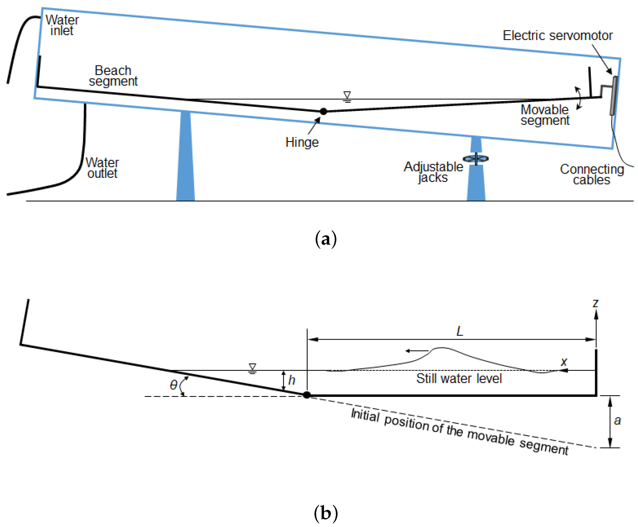
2.1. Physical Model by Lu and Colleagues

Figure 1 illustrates the new bottom-tilting wave generation facility constructed by Lu and colleagues at University of Dundee, UK [24,36,37]. The wave tank was 2 m long, 0.11 m wide, and 0.2 m deep, and one-half of the tank was allowed to rotate about the hinge located at the center of the tank bottom. The 1 m long movable segment was driven by an electric servomotor with a linear motion track installed vertically to move steadily upward or downward in a finite duration. Accordingly, waves with either an elevation or a depression front were generated as demonstrated in Figure 1b. The maximum speed of the equipped servomotor was 1 cm/s in terms of linear motion. The length of the track, and thus the largest vertical excursion, was 0.3 m. However, due to the size limit and the length–depth ratio of the wave tank, in order to avoid the uprunning waves splashing out of the tank the maximum vertical displacement of the movable segment allowed was determined experimentally to be only 4 cm in a very shallow water of a few centimeters. Interested readers are referred to the works in [24,36] for more details.

Considering purely hydrodynamic responses, common properties of the generated waves, such as wave amplitude $\left(A_w\right)$, wave period $\left(T_w\right)$, and wavelength $\left(L_w\right)$, are clearly controlled by the length of the movable segment, L, and two bottom motion parameters a and b, which represent, respectively, the magnitude of vertical disparagement at the endpoint of the moving bottom (i.e., $x=0$, see Figure 1b for the coordinate system) and the duration of bottom motion. In the experiments, the motion of the movable segment, $0<x<L=1$ m, was prescribed explicitly in terms of its vertical displacement, ${\zeta }_m$, as [38]

$${\zeta }_m(x,t)=\left(-a+\frac{a}{b}t\right)\frac{L-x}{L},0<t<b$$

(1)

for leading elevation waves and

$${\zeta }_m(x,t)=\left\{\begin{array}{cc}\hfill -\frac{a}{b}t\frac{L-x}{L},& 0<t<b\hfill \\ \hfill -a+\frac{a}{b}\left(t-b\right)\frac{L-x}{L},& b<t<2b\hfill \end{array}\right.$$

(2)

for leading depression waves. Under various values of b, the trends of wave amplitude $A_w$ versus a and the wave period $T_w$ versus a have been illustrated using experimental measurements [37]. In addition, an explicit formula for $A_w$ as a function of the volume flux of water displaced by per unit width of the wavemaker, $aL/2b$, has been reported as [36]

$$A=m{\left(\frac{aL}{2b}\right)}^n,(m,n)=\left\{\begin{array}{cc}\hfill & (0.06547,-0.4994)(\mathrm{Leading}\mathrm{elevation})\hfill \\ \hfill & (0.09224,-0.4380)(\mathrm{Leading}\mathrm{depression})\hfill \end{array}\right..$$

(3)

We note that the above result was obtained under $L=1$ m, a = 0.005∼ 4 cm, and b = 0.5∼2 s. The limited values of a and b are restricted by the size of the wave tank. To explore the possible use of the new wavemaker, we shall discuss the wave conditions under a wider range of $(L,a,b)$. Furthermore, we shall also examine the waveform of the produced waves since tsunami runup is one of the most popular subjects in tsunami research and it has been confirmed that the shape of the waves is a key control parameter affecting the runup process [48]. We will employ a RANS-based numerical model to address all these issues and the details are to be presented in the following sections.

2.2. Numerical Model for Bottom-Tilting Wavemaker

Numerical simulations of bottom-tilting wavemaker will be performed by a computer model implementing Reynolds-averaged Navier–Stokes (RANS) equations. The model is based on an open source software olaFlow CFD Suite [40], a wave modeling toolbox developed based on the popular OpenFOAM software package [46]. Some of the most important features provided by olaFlow are the numerical treatments for the issues commonly appeared in numerical simulation of wave problems, such as wave generation, moving domain, and absorbing boundary [45]. Furthermore, olaFlow has been employed to successfully study geophysical tsunami waves [11]. We note that olaFlow has been designed capable of simulating two-phase flow through porous media, the RANS-based continuity equation and momentum equations that it solves are summarized as [40]

$$\frac{\partial \langle u_i\rangle }{\partial x_i}=0$$

(4)

and

$$\begin{array}{c}\hfill \frac{1+C}{\varphi }\frac{\partial \rho \langle u_i\rangle }{\partial t}+\frac{1}{\varphi }\frac{\partial }{\partial x_j}\left[\frac{1}{\varphi }\rho \langle u_i\rangle \langle u_j\rangle \right]=-\frac{\partial {\langle p^{*}\rangle }^f}{\partial x_i}-g_i{X}_j\frac{\partial \rho }{\partial x_i}+\frac{1}{\varphi }\frac{\partial }{\partial x_j}\left[{\mu }_{\mathrm{eff}}\frac{\partial \langle u_i\rangle }{\partial x_j}\right]+F_i^{ST}\\ \hfill -\alpha \frac{{\left(1-\varphi \right)}^3}{{\varphi }^3}\frac{\mu }{D_{50}^2}\langle u_i\rangle -\beta \left(1+\frac{7.5}{\mathrm{KC}}\right)\frac{1-\varphi }{{\varphi }^3}\frac{\rho }{D_{50}}\sqrt{\langle u_j\rangle \langle u_j\rangle }\langle u_i\rangle ,\end{array}$$

(5)

respectively. In the above, t is time, $\langle u_i\rangle$ denotes the averaged velocity component in the corresponding $x_i$ direction, ${\langle p^{*}\rangle }^f$ the averaged pseudodynamic pressure, $\rho$ the fluid density, ${\mu }_{\mathrm{eff}}$ the effective dynamic viscosity, $g_i$ the gravitational acceleration, $X_j$ the position vector, and C the added mass coefficient. Effects of surface tension, represented by the $F_i^{ST}$ term, will not be considered. We note that the porosity is taken as $\varphi =1$ as we are not dealing with flow in porous medium. Consequently, both terms in the last line of (5) are also neglected. The above equations are solved with a predictor–corrector method using the PIMPLE algorithm, a combination of PISO (Pressure Implicit with Splitting of Operator) and SIMPLE (Semi-Implicit Method for Pressure-Linked Equations) schemes [40]. With regard to the treatment of the free surface between water and air, the volume of fluid technique is adopted and the associated advection equation is

$$\frac{\partial {\alpha }_f}{\partial t}+\frac{\partial \langle {\alpha }_f{u}_i\rangle }{\partial x_i}=0,$$

(6)

where ${\alpha }_f$ is the so-called fraction function of the water phase and again $\varphi =1$ for our problem. We note that the typical VOF approach has some known issues, such as grid resolution requirement and the problem with possible parasitic currents [41]. However, as evident by the successful application of olaFlow to study tsunami wave hydrodynamics [11,47], which is directly related our problem involving wave propagation and wave runup, we believe that the well-validated olaFlow is a proper tool for our numerical study on bottom-tilting wavemaker. Detailed derivation and procedures for numerical solutions can be obtained in [40].

We are developing a numerical version of the bottom-tiling wavemaker shown in Figure 1 to investigate the wave generation characteristics of this type of wave generator. In our simulations, no traditional wave generation mechanism is required. However, the motion of the bottom movable segment will need to be prescribed according to (1) and (2), while typical wall boundary conditions are implemented for the rest of the boundary. The bottom motion is prescribed by allowing the movable segment to rotate at a constant speed about the hinge point and matching the velocity of the fluid attached to the wavemaker to the velocity of the moving bottom using a simple supplement algorithm that we have developed. To examine the performance of the numerical model and to test the required temporal and spatial resolutions, two related cases have been considered. The first one is to simulate the tsunami waves generated by an idealized rectangular block of size $h_r$-by-$w_r$ erecting abruptly from the ocean bottom in a constant depth $h_0$. Figure 2 shows the free-surface profile of the wave train due to a rectangular disturbance with $h_r$ = 0.05 m and $w_r$ = 12.2 m. As can be seen in the figure, our simulated results agree reasonably with the existing solutions obtained by solving Boussinesq equations [25]. The second case is to compare our simulated results with the experimental data reported by Lu, Park, and Cho [37]. Figure 3 shows the records of free-surface elevation measured at the hinge due to the imposed bottom motion by (1) for a leading elevation wave and (2) for a leading depression wave. In the experiment, $a=0.02$ cm, $b=1$ s, the initial water depth at the hinge was $h_0=0.03$ m, and the beach slope was 1:20. Virtually, the comparison between our results and the laboratory data shows a fair agreement, as suggested by the examples demonstrated in Figure 3. We note that Lu, Park, and Cho [37] also presented their numerical results based on nonlinear shallow water equations with an ad hoc quadratic drag term to account for bottom friction. A drag coefficient of $C_d=0.025$ was used in their calculations and their numerical solutions are also plotted in Figure 3 for reference. We are unable to evaluate whether the value of $C_d$ would significantly affect their numerical results. However, judging from the reasonable agreements with the measurements for both leading elevation and leading depression waves we are comfortable with our results.

3. Results

In this section, we will use the olaFlow-based numerical model that has been discussed and validated in Section 2.2 to simulate a numerical wave tank equipped with a bottom-tilting wavemaker. Characteristics of surfaces waves generated by a bottom-tilting wavemaker will be investigated. Specifically, we will discuss how the input parameters including the length of the moving bottom (L), magnitude of vertical displacement (a), bottom motion duration (b), and water depth at the hinge ($h_0$), on the wave parameters of the produced waves, namely, wavelength ($L_w$), wave amplitude ($A_w$), and phase speed $\left(c_w\right)$. In our simulations, we shall use the free-surface records at the hinge to calculate these wave parameters as suggested by Lu [24]. We will not elaborate the detailed procedure here.

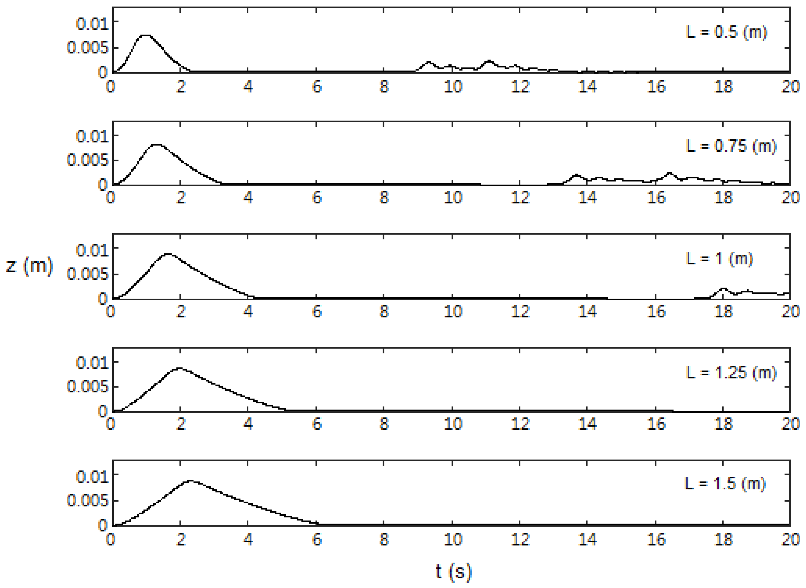
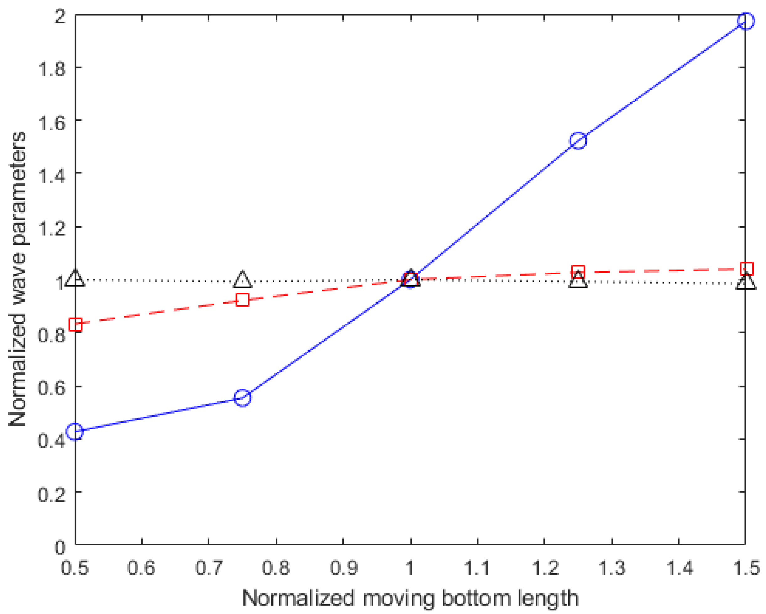
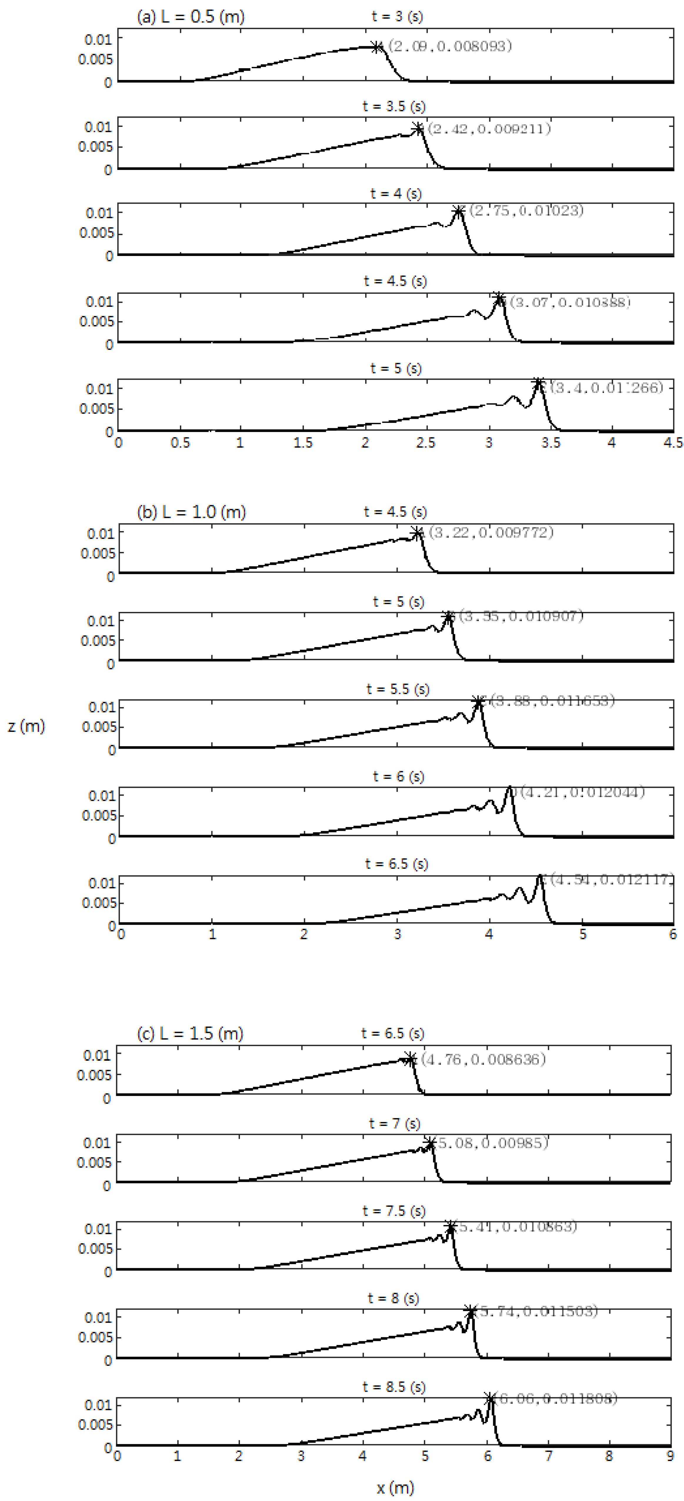
3.1. Effects of Moving Bottom Length, L

We consider waves generated by different lengths of moving bottom. For convenience of comparison, we adopt the following laboratory conditions,

$$h_0=0.03\mathrm{m},a=0.02\mathrm{m},b=0.5\mathrm{s}$$

but let $L=0.5,0.75,1,1.25,1.5$ m. A flat beach is considered (i.e., $\theta =0$, see Figure 1b) and the total length of the wave tank is set to be $6L$ to ensure a sufficient propagation distance for the produced waves to evolve. Leading elevation waves are expected as the upward bottom motion described by (1) will be imposed in our simulations. Figure 4 shows the free-surface elevations recorded at the hinge under five different values of L. The corresponding wave parameters are also summarized in

Table 1. Effects of wavemaker length, L: wave parameters of leading elevation waves due to wavemakers of varying lengths. Bottom motion is given in (1) with $a=0.02$ m and $b=0.5$ s and the constant water depth is $h_0=0.03$ m. The corresponding free-surface records at the hinge are plotted in Figure 4.

Wavemaker Length	Wavelength	Wave Amplitude	Phase Speed
L (m)	${\mathit{L}}_{\mathit{w}}$ (m)	${\mathit{A}}_{\mathit{w}}$ (mm)	${\mathit{c}}_{\mathit{w}}$ (m/s)
0.50	1.80	7.35	0.660
0.75	2.44	8.13	0.655
1.00	4.40	8.82	0.660
1.25	6.70	9.06	0.655
1.50	8.68	9.17	0.650

. The numerical solutions suggest that wavelength ($L_w$) grows significantly as the length of wavemaker (L) increases while wave amplitude ($A_w$) increases only slights with the increasing of L. For the phase speed ($c_w$), it remains more or less the same since the variation of $A_w$ is small. We note that $c_w$ are all greater than the linear phase speed, $\sqrt{g{h}_0}=0.54$ m/s, as values of the wave nonlinearity, $A_w/h_0$, are all considerably large. Variations of wave parameters with respect to the moving bottom length are more obviously shown in Figure 5, which represents the results in a normalized manner.

In Figure 6, we plot the evolution of leading elevation waves generated by bottom motion (1) on a constant depth $h_0=0.03$ m. Three cases with different values of wavemaker length, $L=0.5,1.0,1.5$ m, are presented. We observe that these wave trains grow continuously in terms of both wavelength and wave amplitude, and they begin to disintegrate into several waves at large time as evident by the appearance of multiple leading peaks (see the last panel of each case in Figure 6). We note that this feature is similar to the disintegration of long waves due to an initial static disturbance on the free surface that has been discussed extensively in literature [25]. Furthermore, it can be expected that these leading waves would eventually disintegrate into many separated solitons [49]. Regrading the specific impacts of L on the waveform, comparing three cases presented in Figure 6 we notice that the leading wave becomes more becomes much more asymmetric with the increasing of L, whereas the leading peak does not vary significantly (see also Figure 5).

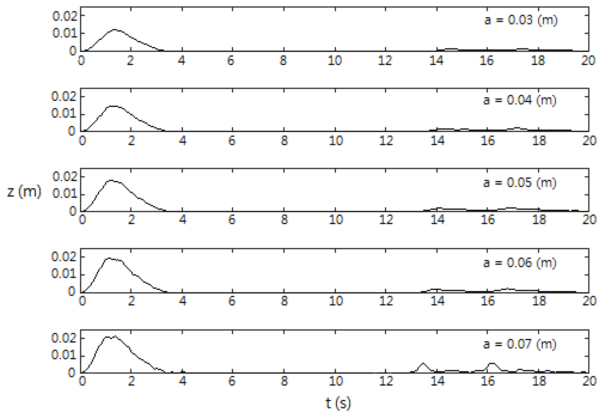
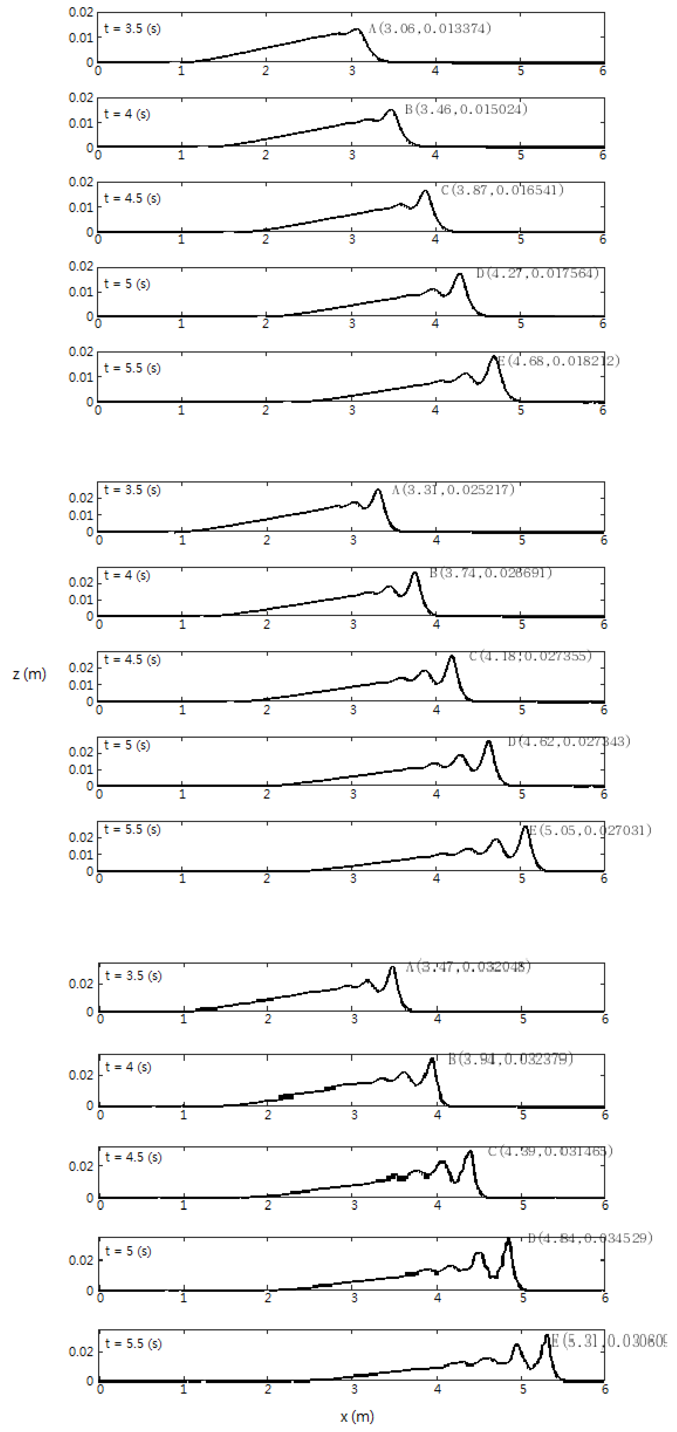
3.2. Effects of Magnitude of Vertical Displacement, a

We now turn our attention to the influence of the magnitude of vertical disparagement at the endpoint of the moving bottom, a. We consider

$$h_0=0.05\mathrm{m},L=1\mathrm{m},b=0.5\mathrm{s}$$

with five different values of displacement: $a=0.03,0.04,0.05,0.06,0.07$ m. Results are tabulated in

Table 2. Effects of vertical displacement of movable segment, a: wave parameters of leading elevation waves due to wavemakers of varying lengths. Bottom motion is given in (1) with $L=1$ m and $b=0.5$ s and the constant water depth is $h_0=0.05$ m. Records of free-surface elevation at the hinge are plotted in Figure 8.

Wavemaker Displacement	Wavelength	Wave Amplitude	Phase Speed
a (m)	${\mathit{L}}_{\mathit{w}}$ (m)	${\mathit{A}}_{\mathit{w}}$ (mm)	${\mathit{c}}_{\mathit{w}}$ (m/s)
0.03	3.00	12.50	0.81
0.04	3.10	15.01	0.84
0.05	3.28	17.98	0.87
0.06	3.55	19.99	0.88
0.07	3.97	21.25	0.90

with the graphical presentation given in Figure 7. The corresponding free-surface elevations recorded at the hinge are also plotted in Figure 8. As can be seen, both wave amplitude $A_w$ and phase speed $c_w$ grow, roughly linearly, with the increasing of wavemaker displacement a, which is expected. However, $A_w$ shows a much greater growth rate. On the other hand, the influence of a on wavelength $L_w$ is comparably less than its impact on $A_w$ as shown in Figure 7.

Figure 9 demonstrates the effects of a on the evolution of waveform. The overall feature is similar to the disintegration process and wave asymmetry shown in Figure 6. However, the separation of leading peaks is more obviously seen, especially for larger a.

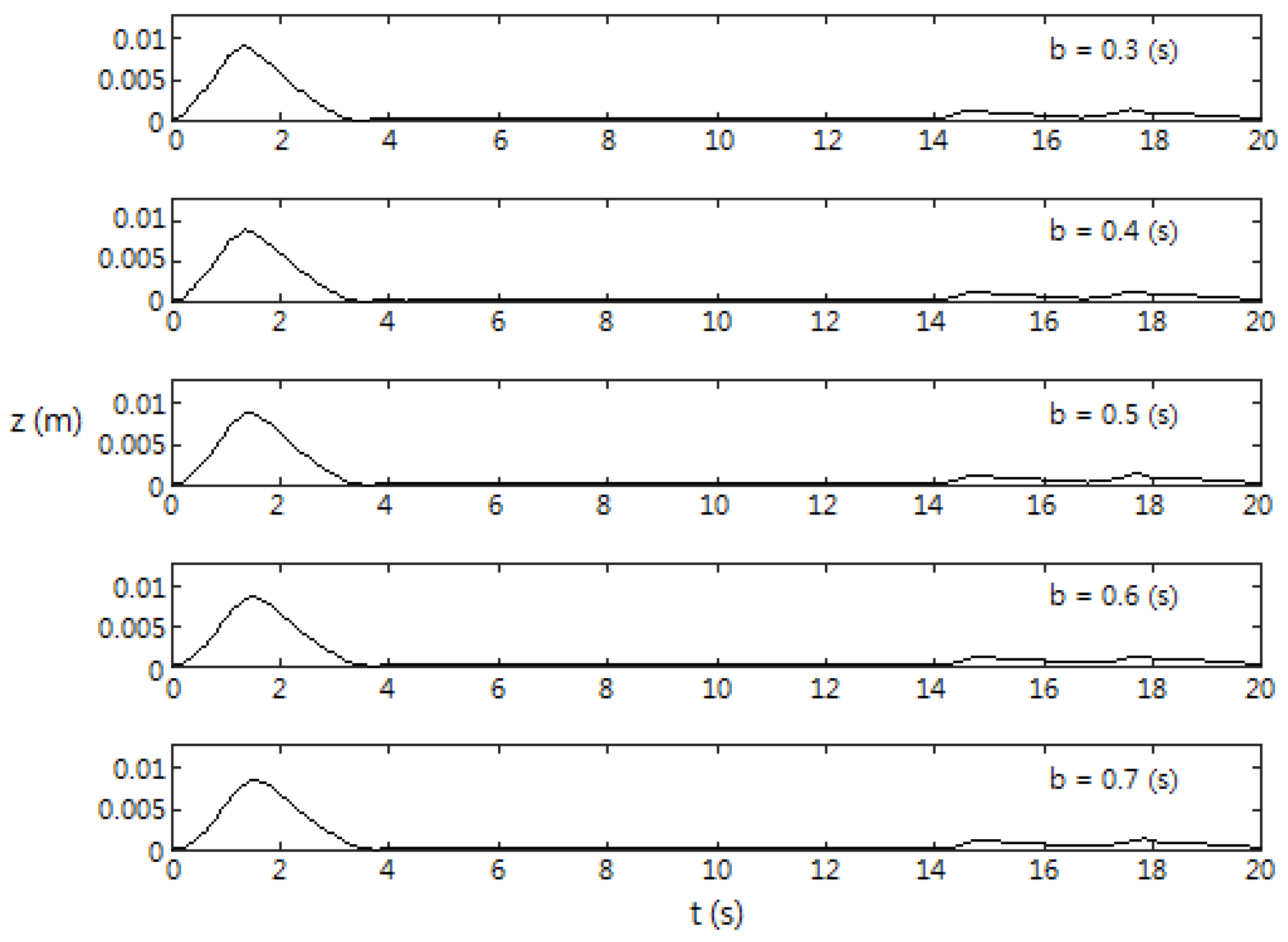
3.3. Effects of Motion Duration, b

Effects of time duration of bottom motion b on the wave generation process are now discussed. In this case, we use five different b values, $b=0.3,0.4,0.5,0.6,0.7$ s while fixing $h_0=0.05$ m, $L=1$ m, and $a=0.02$ m. The simulated free-surface elevation recorded at the hinge is plotted in Figure 10. As can be observed, comparing to the effects of both L and a (see Section 3.1 and Section 3.2), b wave parameters seem to be less sensitive to the motion duration b for the range of values discussed here. We note that rupture velocities for tsunami earthquakes are typically a couple order of magnitudes smaller than the speed of tsunami waves. Consequently, in numerical modeling of tsunami waves the initial water surface profile is is assumed to be the same as the seafloor displacement [9]. Although the motion duration relevant to our problem shall remain small, if we push b to a very large value we can expect only tiny waves being generated, or essentially the slowly rising of water level is observed.

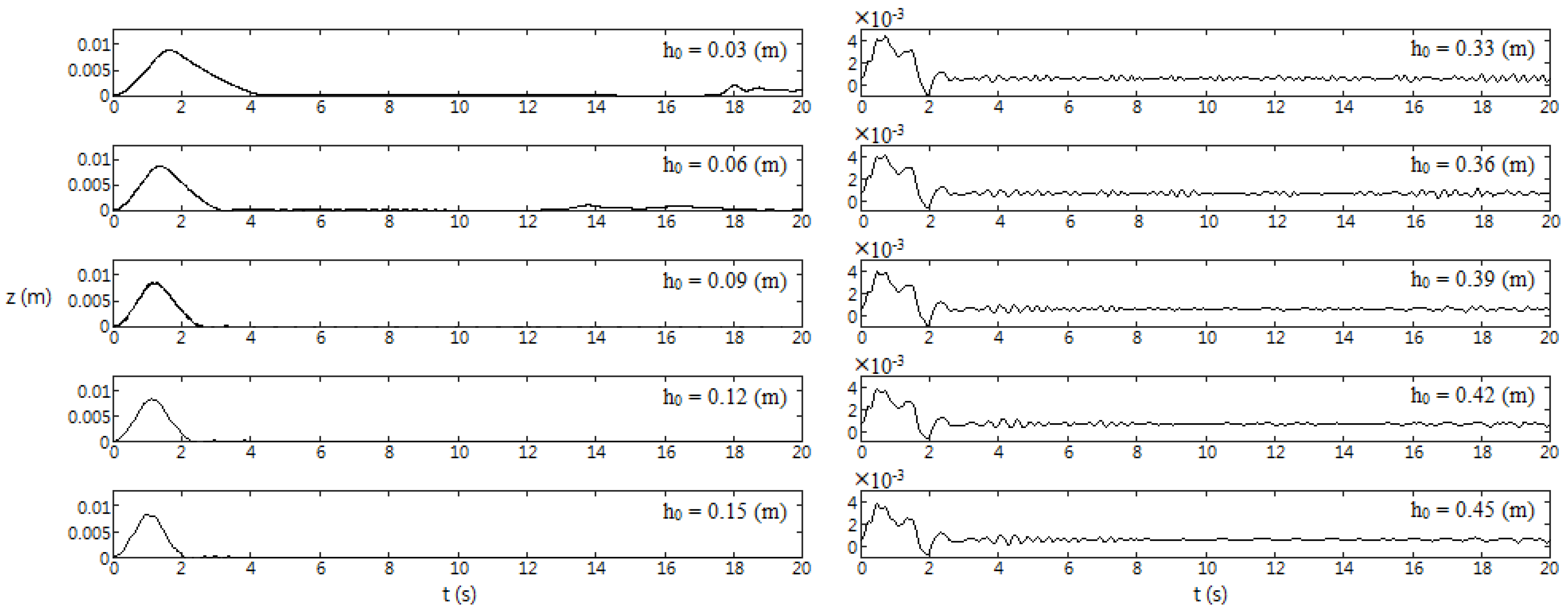
3.4. Effects of Water Depth, $h_0$

Finally, we discuss the effects of initial constant water depth $h_0$ on the wave generation process. We acknowledge that the bottom-tilting wavemaker proposed by Lu and colleagues was originally designed to study waves of very long wavelengths [36]. For the sake of scientific curiosity, we will adopt the water depth even in the range of deep water waves regime. In our simulations, $L=1$ m, $a=0.02$ m, and $b=0.5$ s remain unchanged and the water depth is taken to be $h_0=0.03,0.06,0.09,0.12,0.15,0.33,0.36,0.39,0.45$ m. The correspond simulated free-surface profile recorded at the hinge is plotted in Figure 11 for every $h_0$. For water depth ranges from 0.03 m to 0.15 m, $L_w$ decreases gradually as $h_0$ increases while $A_w$ remains more or less the same. In addition, a single leading elevation peak is distinctly shown. On the other hand, for $h_0=0.33$ to 0.45 m, results in Figure 11 suggest that both wavelength and wave amplitude display little dependence on $h_0$. Furthermore, the leading elevation waves are now consist of a few peaks with small shorter waves riding at the main front and tailing in the back. This is in agreement with the behaviors of waves generated by an impulsive disturbance on surface reported in literature and the known characteristics of long and short waves in the classical water wave theory [25].

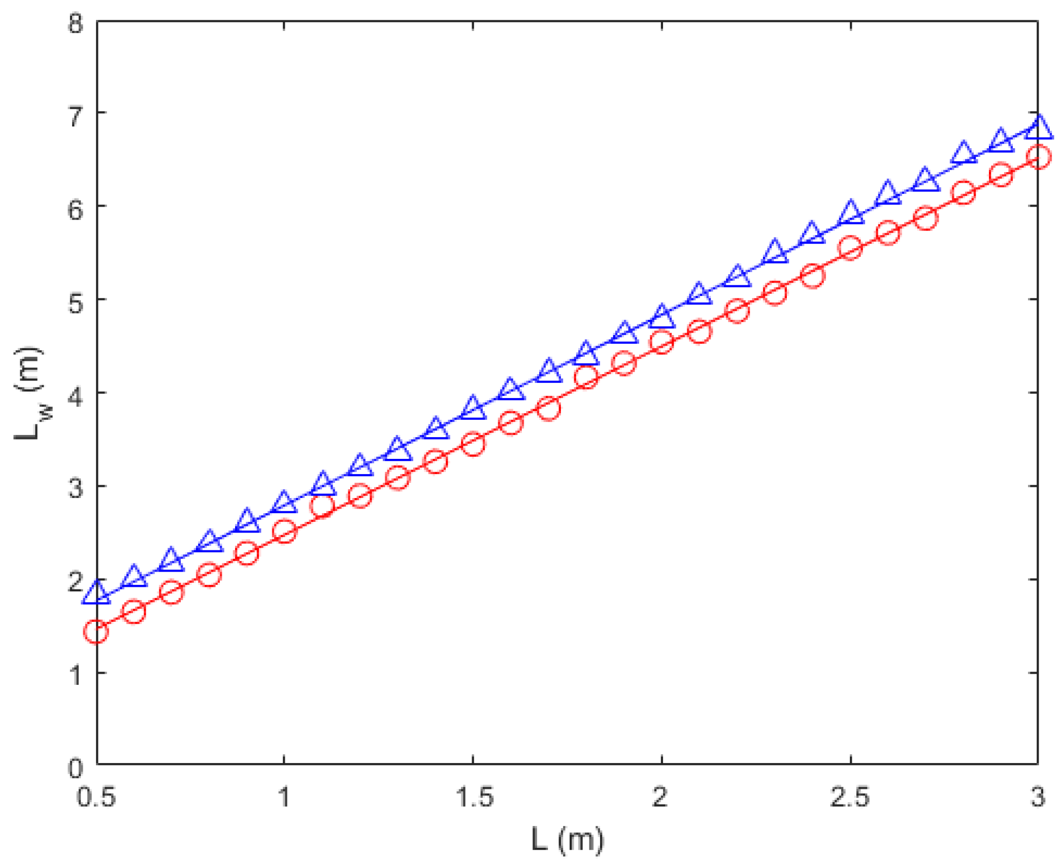
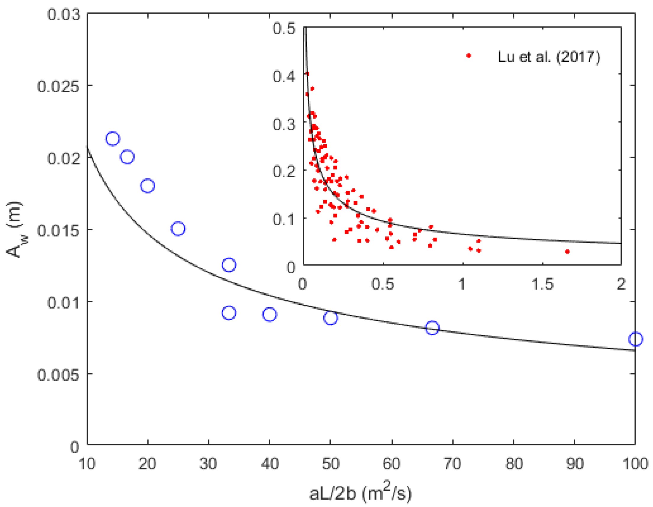
3.5. Wavelength and Wave Amplitude

To gain more insight on the dominate control parameter for wavelength $L_w$, we perform more simulations using the following two sets of parameters.

$$\begin{array}{c}\hfill \mathrm{Set}\mathrm{I}:h_0=0.03\mathrm{m},a=0.02\mathrm{m},b=0.5\mathrm{s},L=0.5\mathrm{to}3\mathrm{m}\\ \hfill \mathrm{Set}\mathrm{II}\text{:}{h}_0=0.05\mathrm{m},a=0.05\mathrm{m},b=1.0\mathrm{s},L=0.5\mathrm{to}3\mathrm{m}\end{array}.$$

In both cases, upward motion described by (1) is considered. Figure 12 summarizes the result from a total of 52 simulations. We observe a simple linear trend, which suggests that $L_w\approx 2L$.

With regard to the wave amplitude $A_w$, Figure 13 plots the computed $A_w$ as a function of $aL/2b$, the volume flux of water displaced by per unit width of the moving bottom, as suggested by Lu, Park, and Cho [36]. We recall a fitted equation proposed by them, i.e., (3), has also been plotted in the same figure for comparison. We observe from Figure 13 that our numerical results fit reasonably with the predicted $A_w$ by (3). In our numerical simulations, $aL/2b$ ranges from 10 to 100 m${}^2$/s and the corresponding $A_w$ is between 0.005 and 0.025 m, as can be seen in Figure 13. However, the fitting coefficients m and n required in (3), the formula for $A_w$, were obtained using results with $aL/2b$ between 0 and 2 [36] (see the upper corner plot in Figure 13). It is surprising but very encouraging that (3) can be extended to estimate the produced wave amplitude for quite a wide range of $aL/2b$ value.

4. Concluding Remarks

Inspired by the bottom-tilting wavemaker proposed by Lu and colleagues for tsunami research, we perform numerical wave tank experiments to facilitate a better understanding of the generation and control mechanisms of the new wavemaker, where waves are generated by the tilting of the movable tank bottom. The numerical tool we employ is an olaFlow-based model implementing Reynolds-averaged Navier–Stokes equations with an simple algorithm that we develop to describe the rotational motion of bottom-tilting wavemaker. Through our simulations, we specifically discuss the effects of input parameters, namely, the length of the moving bottom (L), magnitude of its vertical displacement (a), bottom motion duration (b), and the initial constant water depth ($h_0$), on the typical wave parameters of the produced waves including wavelength ($L_w$), wave amplitude ($A_w$), and phase speed $\left(c_w\right)$. We believe that we obtain some encouraging results through our analysis. The following points are reached based on the observations from our numerical experiments.

• Effects of wavemaker length, L (Section 3.1): $L_w$ grows rapidly as L increases while both $A_w$ and $c_w$ are not too sensitive to the change of L.
• Effects of bottom vertical displacement, a (Section 3.2): $L_w$, $A_w$, and $c_w$ all increase with the increasing of a. However, a has the most dominate effect on $A_w$.
• Effects of motion duration, b (Section 3.3): Within the range of b values that we have discussed, b has little control over $L_w$, $A_w$, and $c_w$.
• Effects of water depth, $h_0$ (Section 3.4): For shallower depth, $L_w$ decreases as $h_0$ increases. However, $h_0$ does not affect $L_w$ for relative deeper water. In both depth regimes, $A_w$ is unaffected by the change of $h_0$.
• Wavelength, $L_w$, and wave amplitude, $A_w$ (Section 3.5): $L_w$ depends linearly on L, $Lw\approx 2L$. $A_w$ is a function of $aL/2b$ and the fitted Equation (3) is applicable for a wide range of $aL/2b$ value.

Through the above results, we now have a better knowledge on the generation algorithm of the bottom-tiling wavemaker. Using the these relationships, we are able to control the wave parameters of the produced waves. This certainly makes the newly designed bottom-tilting generator more useful for tsunami research.

As bottom-tilting wavemaker bears no inherent wavelength-stork constraint and can generate longer waves comparing to the widely used piston-type wavemakers in typical laboratory setting, we suggest that the new wave generator indeed has the potential to serve as the next-generation laboratory facility specifically for tsunami research. The findings from our study can help understand much better the control of wave generation using the new wavemaker. Nevertheless, there are still many challenges to meet in order to adopt this new kind of technique for practical use for tsunami research. One particular aspect that probably still requires some more attention is the prediction of the waveform of leading waves generated by bottom-tilting wavemaker. In our analysis, we have successfully demonstrated numerically the evolution of leading waves. However, it is not straightforward to describe the shape of the leading waves in a similar manner to some well-known wave theories, such as sinusoidal waves and solitary wave, who use simple expressions for the waveform. Presumably if the wave nonlinearity is weak, the solution technique to the linear KdV equation can be applied to deduce the asymptotic solution for the waveform [25]. However, when the wave nonlinearity becomes considerable it is probably impossible to obtain an analytic form. In such case, we will need to turn to numerical approach, like we have demonstrated in Section 3.

The fundamental idea behind bottom-motion type wave generators is simple and is directly related to the source mechanism of earthquake-generated tsunamis. However, they seem to be less commonly used in laboratory study for wave hydrodynamics. There are a few of similar types of wavemaker that have been reported in literature. In particular, we mentioned one of the pioneering work by Hammack and Segur [49], who used a rectangular piston located in the tank bed as the wave generator to study waves caused by an impulsive motion of the seabed. Interested reads are referred to their work.

Finally, we reiterative that only the hydrodynamic problem has been considered in our study. We have boldly ignored any possible mechanical and electrical issues that can never be avoided in laboratory studies. We acknowledge that these issues can be the most time-consuming and troublesome tasks and probably have no less weighting than any other elements in the laboratory study of coastal wave problems.

References

1. Okal, E.A. The quest for wisdom: Lessons from 17 tsunamis, 2004–2014. Philos. Trans. R. Soc. A 2015, 373, 20140370. [Google Scholar] [CrossRef] [PubMed]
2. Imamura, F.; Boreta, S.P.; Suppasri, A.; Muhari, A. Recent occurrences of serious tsunami damage and the future challenges of tsunami disaster risk reduction. Prog. Disast. Sci. 2019, 1, 100009. [Google Scholar] [CrossRef]
3. Widiyanto, W.; Santoso, P.B.; Hsiao, S.-C.; Imananta, R.T. Post-event field survey of 28 September 2018 Sulawesi earthquake and tsunami. Nat. Hazards Earth Syst. Sci. 2015, 19, 2781–2794. [Google Scholar] [CrossRef] [Green Version]
4. Wallemacq, P.; Below, R.; McLean, D. UNISDR and CRED Report: Economic Losses, Poverty & Disasters (1998–2017); United Nations Office for Disaster Risk Reduction: Geneva, Switzerland, 2018. [Google Scholar]
5. Synolakis, C.E.; Bernard, E.N. Tsunami science before and beyond Boxing Day, 2004. Philos. Trans. R. Soc. A 2006, 364, 2231–2265. [Google Scholar] [CrossRef] [PubMed]
6. Satake, K. Advances in earthquake and tsunami sciences and disaster risk reduction since the 2004 Indian ocean tsunami. Geosci. Lett. 2014, 1, 15. [Google Scholar] [CrossRef] [Green Version]
7. Rabinovich, A.B.; Geist, E.L.; Fritz, H.M.; Borrero, J.C. Introduction to “Tsunami Science: Ten Years after the 2004 Indian Ocean Tsunami. Volume I”. Pure Appl. Geophys. 2015, 172, 615–619. [Google Scholar] [CrossRef] [Green Version]
8. Heidarzadeh, M.; Muhari, A.; Wijanarto, A.B. Insights on the source of the 28 September 2018 Sulawesi tsunami, Indonesia based on spectral analyses and numerical simulations. Pure Appl. Geophys. 2019, 176, 25–43. [Google Scholar] [CrossRef] [Green Version]
9. Wang, X.; Liu, P.L.-F. Numerical simulations of the 2004 Indian Ocean tsunamis—Coastal effects. J. Earthq. Tsunami 2007, 1, 273–297. [Google Scholar] [CrossRef]
10. Fritz, H.M.; Mohammed, F.; Yoo, J. Lituya Bay landslide impact generated mega-tsunami 50th anniversary. Pure Appl. Geophys. 2009, 166, 153–175. [Google Scholar] [CrossRef]
11. Liu, P.L.-F.; Higuera, P.; Husrin, S.; Prasetya, G.S.; Prihantono, J.; Diastomo, H.; Pryambodo, D.G.; Susmoro, H. Coastal landslides in Palu Bay during 2018 Sulawesi earthquake and tsunami. Landslides 2020, 17, 2085–2098. [Google Scholar] [CrossRef]
12. Carrier, G.F.; Greenspan, H.P. Water waves of finite amplitude on a sloping beach. J. Fluid Mech. 1958, 4, 97–109. [Google Scholar] [CrossRef]
13. Madsen, P.A.; Schäffer, H.A. Analytical solutions for tsunami runup on a plane beach: Single waves, N-Waves Transient Waves. J. Fluid Mech. 2010, 645, 25–57. [Google Scholar] [CrossRef]
14. Liu, P.L.-F.; Cho, Y.-S.; Yoon, S.B.; Seo, S.N. Numerical simulations of the 1960 Chilean tsunami propagation and inundation at Hilo, Hawaii. In Recent Developments in Tsunami Research; El-Sabh, M.I., Ed.; Kluwer Academic Publishers: Dordrecht, The Netherlands, 1994; pp. 99–115. [Google Scholar]
15. Titov, V.; Kânoğlu, U.; Synolakis, C. Development of MOST for real-time tsunami forecasting. J. Waterw. Port. Coast. 2016, 142, 03116004. [Google Scholar] [CrossRef]
16. Synolakis, C.E. The runup of solitary waves. J. Fluid Mech. 1987, 185, 523–545. [Google Scholar] [CrossRef]
17. Liu, P.L.-F.; Wu, T.-R.; Raichlen, F.; Synolakis, C.E.; Borrero, J.C. Runup and rundown generated by three-dimensional sliding masses. J. Fluid Mech. 2005, 536, 107–144. [Google Scholar] [CrossRef] [Green Version]
18. Madsen, O.S. On the generation of long waves. J. Geophys. Res. 1971, 76, 8672–8683. [Google Scholar] [CrossRef]
19. Synolakis, C.E. Generation of long waves in laboratory. J. Waterw. Port. Coast. 1990, 116, 252–266. [Google Scholar] [CrossRef]
20. Kaplan, K. Generalized Laboratory Study of Tsunami Run-Up; Tech. Memo 60; Beach Erosion Board, U.S. Army Corps of Engineers: Vicksburg, MS, USA, 1995. [Google Scholar]
21. Li, Y. Tsunamis: Non-Breaking and Breaking Solitary Wave Run-Up. Ph.D. Thesis, California Institute of Technology, Pasadena, CA, USA, 2000. [Google Scholar]
22. Synolakis, C.E.; Deb, M.K.; Skjelbreia, J.E. The anomalous behavior of the run-up of cnoidal waves. Phys. Fluids 1998, 31, 3–5. [Google Scholar] [CrossRef]
23. Lima, V.V.; Avilez-Valente, P.; Baptista, M.A.V.; Miranda, J.M. Generation of N-waves in laboratory. Coast. Eng. 2019, 148, 1–18. [Google Scholar] [CrossRef]
24. Lu, H. Generation of Very Long Waves in Laboratory for Tsunamis Research. Ph.D. Thesis, University of Dundee, Dundee, UK, 2017. [Google Scholar]
25. Madsen, P.A.; Fuhrman, D.R.; Schäffer, H.A. On the solitary wave paradigm for tsunamis. J. Geophys. Res. 2008, 113, C12012. [Google Scholar] [CrossRef]
26. Van Gent, M.R.A. The new delta flume for large-scale testing. In Proceedings of the 36th IAHR World Congress, The Hague, The Netherlands, 28 June–3 July 2015. [Google Scholar]
27. Zhang, H.; Geng, B. Introduction of the world largest wave flume constructed by TIWTE. In Proceedings of the APAC 2015, Chennai, India, 7–10 September 2015. [Google Scholar]
28. Schimmels, S.; Sriram, V.; Didenkulova, I. Tsunami generation in a large scale experimental facility. Coast. Eng. 2016, 110, 32–41. [Google Scholar] [CrossRef]
29. Allsop, W.; Robinson, D.; Charvet, I.; Rossetto, T.; Abernethy, R. A unique tsunami generator for physical modelling of violent flows and their impact. In Proceedings of the 14th World Conference of Earthquake Engineering, Beijing, China, 12–17 October 2008. [Google Scholar]
30. Rossetto, T.; Allsop, W.; Charvet, I.; Robinson, D. Physical modelling of tsunami using a new pneumatic wave generator. Coast. Eng. 2011, 58, 517–527. [Google Scholar] [CrossRef]
31. Charvet, I. Experimental Modelling of Long Elevated and Depressed Waves Using a New Pneumatic Wave Generator. Ph.D. Thesis, University College London, London, UK, 2011. [Google Scholar]
32. Charvet, I.; Eames, I.; Rossetto, T. New tsunami runup relationships based on long wave experiments. Ocean Model. 2013, 69, 79–92. [Google Scholar] [CrossRef] [Green Version]
33. Goseberg, N.; Wurpts, A.; Schlurmann, T. Laboratory-scale generation of tsunami and long waves. Coast. Eng. 2013, 79, 57–74. [Google Scholar] [CrossRef]
34. Bremm, G.C.; Goseberg, N.; Schlurmann, T.; Nistor, I. Long wave flow interaction with a single square Structure on a sloping beach. J. Mar. Sci. Eng. 2015, 3, 821–844. [Google Scholar] [CrossRef] [Green Version]
35. Drähne, U.; Goseberg, N.; Vater, S.; Beisiegel, N.; Behrens, J. An experimental and numerical study of long wave run-up on a plane beach. J. Mar. Sci. Eng. 2016, 4, 821. [Google Scholar] [CrossRef] [Green Version]
36. Lu, H.; Park, Y.S.; Cho, Y.-S. Investigation of long waves generated by bottom-tilting wave maker. Coast. Eng. J. 2017, 59, 1750018. [Google Scholar] [CrossRef]
37. Lu, H.; Park, Y.S.; Cho, Y.-S. Modelling of long waves generated by bottom-tilting wave maker. Coast. Eng. 2017, 122, 1–9. [Google Scholar] [CrossRef] [Green Version]
38. Lu, H.; Park, Y.S.; Cho, Y.-S. Run-up of long waves generated by bottom-tilting wave maker. J. Hydraul. Res. 2020, 58, 47–59. [Google Scholar] [CrossRef]
39. Goseberg, N. The run-up of long waves—Laboratory-scaled geophysical reproduction and onshore interaction with macro-roughness elements. Ph.D. Thesis, Leibniz Universität Hannover, Hannover, Germany, 2011. [Google Scholar]
40. Higuera, P. Application of Computational Fluid Dynamics to Wave Action on Structures. Ph.D. Thesis, University of Cantabria, Santander, Spain, 2015. [Google Scholar]
41. Ma, G.; Shi, F.; Kirby, J.T. Shock-capturing non-hydrostatic model for fully dispersive surface wave processes. Ocean Model. 2012, 43, 22–35. [Google Scholar] [CrossRef]
42. Derakhti, M.; Kirby, J.T.; Shi, F.; Ma, G. NHWAVE: Consistent boundary conditions and turbulence modelling. Ocean Model. 2016, 106, 121–130. [Google Scholar] [CrossRef]
43. Gallerano, F.; Cannata, G.; Barsi, L.; Palleschi, F.; Iele, B. Simulation of wave motion and wave breaking induced energy dissipation. WSEAS Trans. Fluid Mech. 2019, 14, 62–69. [Google Scholar]
44. Gallerano, F.; Cannata, G.; Barsi, L.; Palleschi, F. Hydrodynamic effects produced by submerged breakwaters in a coastal area with a curvilinear shoreline. J. Mar. Sci. Eng. 2019, 7, 337. [Google Scholar] [CrossRef] [Green Version]
45. Higuera, P.; Losada, I.J.; Lara, J.L. Three-dimensional numerical wave generation with moving boundaries. Coast. Eng. 2015, 101, 35–47. [Google Scholar] [CrossRef]
46. Weller, H.G.; Tabor, G.; Jasak, H.; Fureby, C. A tensorial approach to computational continuum mechanics using object-oriented techniques. Comput. Phys. 1998, 12, 620–631. [Google Scholar] [CrossRef]
47. Higuera, P.; Liu, P.L.-F.; Lin, C.; Wong, W.-Y. Laboratory-scale swash flows generated by a non-breaking solitary wave on a steep slope. J. Fluid Mech. 2018, 847, 186–227. [Google Scholar] [CrossRef]
48. Chan, I.-C.; Liu, P.L.-F. On the runup of long waves on a plane beach. J. Geophys. Res. 2012, 117, C08006. [Google Scholar] [CrossRef]
49. Hammack, J.L.; Segur, H. The Korteweg–de Vries equation and water waves. Part 2. Comparison with experiments. J. Fluid Mech. 1974, 65, 289–314. [Google Scholar] [CrossRef] [Green Version]
Figure 1. (a) Schematic of the 2 m long bottom-tilting wavemaker designed by Lu and colleagues [24,36,37]. redSee in [24] for the detailed design and configuration. (b) Example of a leading elevation wave generated by the movable segment with upward motion. ( x , z ) denotes the coordinate system. θ : beach slope, h: water depth, L: length of the wave generator, a: magnitude of the vertical displacement at x = 0 .
Jmse 08 00769 g001
Figure 2. Surface waves generated by a rectangular disturbance with height h r and width w r : snapshots of free-surface displacement, η , normalized by the constant water depth, h 0 , presented in a moving coordinate. Solid line: present solutions. Dashed line: numerical results by Boussinesq model reported by Madsen, Fuhrman, and Schäffer [25]. Upper and lower panel plot the results at dimensionless time t / h 0 / g = 35 and 90, respectively. In this case, h r / h 0 = 0.1 and w r / h 0 = 24.4. The horizontal and vertical resolutions in our calculations are 0.02 m and 0.009374 m, respectively, and Δ t = 0.01 s is used.
Jmse 08 00769 g002
Figure 3. Records of free-surface elevation measured at the hinge. Top: leading elevation wave due to the upward bottom motion given in (1). Bottom: leading depression wave due to the imposed bottom motion by (2). Our solutions (solid lines) are compared with both numerical (dased lines) and laboratory (dots) results reported by Lu, Park, and Cho [37]. Vertical dotted line indicates the duration of bottom motion, b / ( L / g h 0 ) = 0.54 . In both cases, L = 1 m, h 0 = 0.03 m, a = 0.02 cm, b = 1 s, and θ = 2 . 86 (1:20 slope).
Jmse 08 00769 g003
Figure 4. Records of free-surface elevation at the hinge under different wavemaker lengths, L. In all cases, h 0 = 0.03 m, a = 0.02 m, b = 0.5 s, and θ = 0 . Upward motion described by (1) is used. Length of the moving bottom (top to bottom): L = 0.5 , 0.75, 1, 1.25, 1.5 m.
Jmse 08 00769 g004
Figure 5. Normalized wave parameters as functions of normalized moving bottom length, L / L 0 . Circle: wavelength, L w / L w , 0 ; square: wave amplitude, A w / A w , 0 ; triangle: phase speed, c w / c w , 0 . Subscript 0 indicates the normalization by the corresponding values at L = 1 m (see Table 1). In all cases, h 0 = 0.03 m, a = 0.02 m, b = 0.5 s, θ = 0 , and the upward bottom motion, (1), is imposed.
Jmse 08 00769 g005
Figure 6. Evolution of leading elevation waves due to upward bottom motion with different length of movable segment, L, on a constant depth, h 0 . (a) L = 0.5 m; (b) L = 1.0 m; (c) L = 1.5 m. Peaks are denoted by asterisks and values in the parentheses indicate (time, displacement) at each peak. In all cases, h 0 = 0.03 m, a = 0.02 cm, b = 0.5 s, and θ = 0 .
Jmse 08 00769 g006
Figure 7. Normalized wave parameters vs. normalized magnitude of vertical wavemaker displacement, a / a 0 . Square: wave amplitude, A w / A w , 0 ; circle: wavelength, L w / L w , 0 ; triangle: phase speed, c w / c w , 0 . Subscript 0 indicates the normalization by the corresponding values at a = 0.03 m (see Table 2). In all cases, h 0 = 0.05 m, L = 1 m, b = 0.5 s, θ = 0 , and the upward bottom motion, (1), is imposed.
Jmse 08 00769 g007
Figure 8. Free-surface elevation of leading elevation waves recorded at the hinge under different magnitudes of vertical wavemaker displacement, a. In all cases, h = 0.05 m, L = 1 m, b = 0.5 s, and θ = 0 . Magnitude of vertical displacement (top to bottom): a = 0.03 , 0.04, 0.05, 0.06, 0.07 m.
Jmse 08 00769 g008
Figure 9. Profiles of leading elevation waves due to upward bottom motion with varying vertical wavemaker displacement, a, on a constant depth, h 0 . Top group a = 0.03 m; middle: a = 0.05 m; bottom a = 0.07 m. Values in the parentheses indicate (time, displacement) at each peak. In all cases, h 0 = 0.05 m, L = 1 cm, b = 0.5 s, and θ = 0 .
Jmse 08 00769 g009
Figure 10. Effects of motion duration b on wave generation by an upward bottom motion: records of free-surface elevation at the hinge for different b values. In all cases, h = 0.05 m, L = 1 m, a = 0.02 m, and θ = 0 . Time duration of bottom motion (top to bottom): b = 0.3 , 0.4, 0.5, 0.6, 0.7 s.
Jmse 08 00769 g010
Figure 11. Initial water depth h 0 on wave generation: records of free-surface elevation at the hinge. In all cases, L = 1 m, a = 0.02 m, and b = 0.5 s are used in (1) to describe the bottom motion and a flat beach is consider ( θ = 0 ). Water depth for each case is indicated in the corresponding panel.
Jmse 08 00769 g011
Figure 12. Wavelength L w as functions of moving bottom length L. Circle (Set I): h 0 = 0.03 m, a = 0.02 m, b = 0.5 s. Square (Set II): h 0 = 0.05 m, a = 0.05 m, b = 1 s. Lines show the corresponding linear fitting for 0.5 < L < 3 m. In both case, θ = 0 and the upward bottom motion, (1), is imposed.
Jmse 08 00769 g012
Figure 13. Wave amplitude, A w , as a function of volume flux of water displaced by per unit width of the moving bottom, a L / 2 b . Circle: present numerical results. Line: fitted equation for A w given in (3). The upper corner subplot shows (3) along with the results used to produce (3) by Lu, Park & Cho [24].
Jmse 08 00769 g013