Influence of Mild Bottom Slopes on the Overtopping Flow over Mound Breakwaters under Depth-Limited Breaking Wave Conditions

Abstract

The crest elevation of mound breakwaters is usually designed considering a tolerable mean wave overtopping discharge. However, pedestrian safety, characterized by the overtopping layer thickness (OLT) and the overtopping flow velocity (OFV), is becoming more relevant due to the reduction of the crest freeboards of coastal structures. Studies in the literature focusing on OLT and OFV do not consider the bottom slope effect, even if it has a remarkable impact on mound breakwater design under depth-limited breaking wave conditions. Therefore, this research focuses on the influence of the bottom slope on OLT and OFV exceeded by 2% of incoming waves, h_c,2% and u_c,2%. A total of 235 2D physical tests were conducted on conventional mound breakwaters with a single-layer Cubipod^® and double-layer rock and cube armors with 2% and 4% bottom slopes. Neural networks were used to determine the optimum point to estimate wave characteristics for h_c,2% and u_c,2% calculation; that point was located at a distance from the model toe of three times the water depth at the toe (h_s) of the structure. The influence of the bottom slope is studied using trained neural networks with fixed wave conditions in the wave generation zone; h_c,2% slightly decreases and u_c,2% increases as the gradient of the bottom slope increases.

1. Introduction

Mound breakwater design criteria are evolving due to climate change effects (e.g., sea level rise) and increasing social pressure to reduce the visual impact of coastal structures. These phenomena lead to the reduction of their crest freeboards and an increase of the overtopping hazard. In this context, pedestrian safety becomes relevant due to the recreational activities that take place on the breakwater’s crest (e.g., fishing and photography).

An admissible mean wave overtopping discharge, q (m³/s/m), is usually the criteria considered for design purposes. Nevertheless, Franco et al. [1] suggested that the overtopping hazard should be more directly related to individual overtopping events, rather than mean values. When assessing the overtopping hazard to pedestrians standing on coastal structures during overtopping events, several authors (see Bae et al. [2] and Sandoval and Bruce [3]) have proposed using the overtopping layer thickness (OLT) and the overtopping flow velocity (OFV) as relevant variables.

There is extensive literature on q (see EurOtop 2018 [4] and Molines and Medina [5]) and individual wave overtopping volumes (see Nørgaard et al. [6] and Molines et al. [7]) on mound breakwaters. Nevertheless, few studies have focused on OLT and OFV on dikes (see Schüttrumpf and Van Gent [8]) or on mound breakwaters (see Mares-Nasarre et al. [9]). Those studies [8,9] considered variables related to wave characteristics and structure geometry as significant when estimating OLT and OFV. However, the bottom slope (m) has a significant influence on the type of wave breaking at the toe of the structure. Herrera et al. [10] pointed out that the bottom slope plays an important role in mound breakwater design; in depth-limited breaking-wave conditions, the optimum point where wave characteristics are estimated is relevant for design and needs to be determined.

This research focuses on the bottom slope influence on OLT and OFV during extreme overtopping events on mound breakwaters under depth-limited breaking-wave conditions. Two-dimensional physical tests were performed at the wave flume of the Universitat Politècnica de València (Spain), and data were analyzed using artificial neural networks (NNs). This paper is organized as follows. In Section 2, the variables considered in the formulas given in the literature to estimate OLT and OFV are presented. In Section 3, the experimental setup is presented. In Section 4, the analysis carried out with NNs is described; the optimum point to determine wave characteristics to estimate OLT and OFV is identified, and the bottom slope effect is assessed for both variables. Finally, in Section 5, conclusions are drawn.

2. Literature Review on Overtopping Layer Thickness (OLT) and Overtopping Flow Velocity (OFV)

Schüttrumpf and Van Gent [8] integrated the results of Van Gent [11] (m = 1% and 0.2 ≤ H_s/h_s ≤ 1.4, H_s being the significant wave height at the toe of the structure and h_s the water depth at the toe) and Schüttrumpf et al. [12] (horizontal bottom and 0.1 ≤ H_s/h_s ≤ 0.3) and described the overtopping flow on dike crests using two variables: (1) the OLT on the dike crest exceeded by 2% of the incoming waves, h_c,2%, and (2) the OFV on the dike crest exceeded by 2% of the incoming waves, u_c,2%. These authors also proposed a method to estimate h_c,2% and u_c,2% based on the wave run-up height exceeded by 2% of the incoming waves, Ru_2%, obtained with the formulas proposed by Van Gent [13]. Van Gent [13] considered Ru_2% as a function of the surf similarity parameter or Iribarren number, ξ_s,−1, calculated with H_s and the spectral period T_m−1,0 = m₋₁/m₀, where m_i is the i-th spectral moment, and $m_i={{\displaystyle \int }}_0^{\infty }S\left(f\right)f^i df$, being the wave spectrum S(f). Following the Schüttrumpf and Van Gent [8] method, once Ru_2% is estimated, OLT and OFV on the seaward edge of the dike crest can be obtained: h_A,2%(R_c) = h_A(z_A = R_c) and u_A,2%(R_c) = u_A(z_A = R_c). 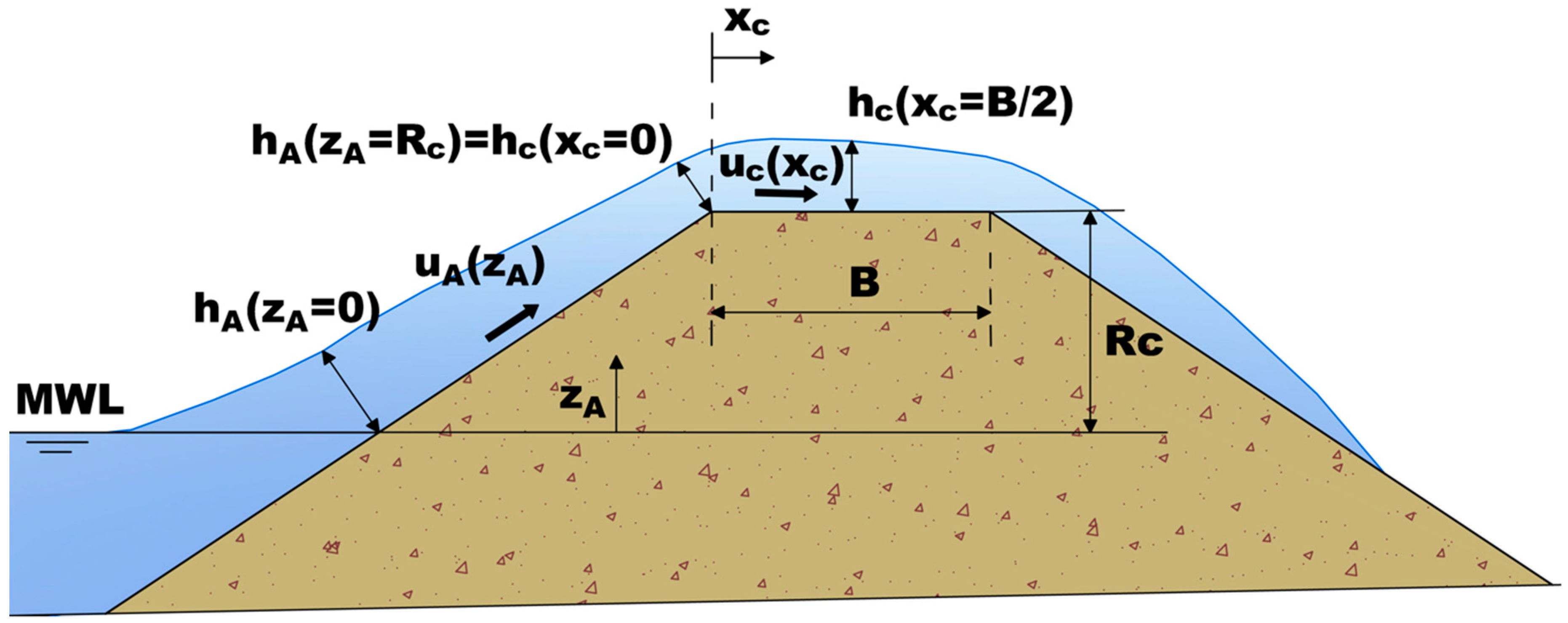Figure 1 shows the variables considered in the model proposed by the aforementioned authors, where MWL is the mean water level.

The OLT and OFV along the seaward slope of the dike depend on the Ru_2% calculated using the formula by Van Gent [13], the elevation over the MWL, z_A, and the significant wave height at the toe of the structure, H_s.

Using the previously calculated values of h_A,2%(z_A = R_c) and u_A,2%(z_A = R_c), OLT and OFV on the crest of the dike, h_c,2% and u_c,2%, are estimated using the distance from the intersection between the seaward slope and the crest, x_c, the crest width, B, and a friction coefficient, µ (see [12] for further guidance on this coefficient).

Van der Meer et al. [14] added their new test observations on dikes (using an overtopping simulator) to the data obtained by Schüttrumpf and Van Gent [8]. Based on the new dataset, Van der Meer et al. [14] proposed a new method to estimate OLT and OFV on dikes; h_A,2% and u_A,2% estimators considered the same variables as Schüttrumpf and Van Gent [8]. The u_c,2% formula included the wavelength based on the spectral period (T_m−1,0), L_m−1,0.

Lorke et al. [15] carried out physical model tests on dikes (horizontal bottom and 0.1 ≤ H_s/h_s ≤ 0.3) focused on the effect of currents and wind on overtopping. Using this dataset, the authors proposed new empirical coefficients for the h_c,2% formulas obtained by Schüttrumpf and Van Gent [8] as a function of the seaward slope of the dike, α.

EurOtop [4] recommended a new method to estimate OLT and OFV on dikes. The formulas to estimate OLT and OFV along the seaward slope are equivalent to those proposed by Schüttrumpf and Van Gent [8] but consider different empirical coefficients. As Lorke et al. [15], EurOtop [4] considers these empirical coefficients as a function of the seaward slope of the dike, α. Regarding u_c,2%, EurOtop [4] suggests the formula given by Van der Meer et al. [14].

Mares-Nasarre et al. [9] adapted the formulas given by Schüttrumpf and Van Gent [8] to estimate h_c,2%(x_c = B/2) on mound breakwaters with m = 2% and 0.2 ≤ H_s/h_s ≤ 0.7. These authors proposed new empirical coefficients and roughness factors for three armor layers (Cubipod^®-1Layer, randomly placed cube-2Layers, and rock-2Layers). Mound breakwaters (permeable structures) and dikes are different structures, but h_c,2%(x_c = B/2) seems to be related to the same variables. Regarding u_c,2%(x_c = B/2), it is calculated as a function of the squared root of h_c,2%(x_c = B/2).

Table 1. Summary of the variables considered for the estimation of OLT and OFV in the literature.

Author		Hs	Tm−1,0	α	Rc	B	µ	Lm−1,0	m
hA,2%	Schüttrumpf and Van Gent [8]	x	x	x
	Van der Meer et al. [14]	x	x	x
	EurOtop [8]	x	x	x
uA,2%	Schüttrumpf and Van Gent [8]	x	x	x
	Van der Meer et al. [14]	x	x	x
	EurOtop [8]	x	x	x
hc,2%	Schüttrumpf and Van Gent [8]	x	x	x	x	x
	Lorke et al. [15]	x	x	x	x
	EurOtop [8]	x	x	x	x
	Mares-Nasarre et al. [9]	x	x	x	x	x
uc,2%	Schüttrumpf and Van Gent [8]	x	x	x	x		x
	Van der Meer et al. [14]	x	x	x	x			x
	EurOtop [8]	x	x	x	x			x
	Mares-Nasarre et al. [9]	x	x	x	x	x

summarizes the variables considered in the models proposed by the aforementioned authors to estimate h_c,2% and u_c,2%.

It can be concluded from Table 1 that only geometric variables of the coastal structure and wave characteristics at the structure toe were considered in the formulations given in the literature to estimate h_c,2% and u_c,2%. Even if Van Gent [11], Schüttrumpf and Van Gent [8], and van der Meer et al. [14] were considering physical tests under depth-limited breaking-wave conditions, none of them considered the bottom slope (m) as a significant variable or analyzed the optimum point for measuring wave characteristics. Here, the optimum point to estimate incident wave characteristics is considered to be the point where the error in the estimation of OLT and OFV is lowest.

3. Experimental Methodology

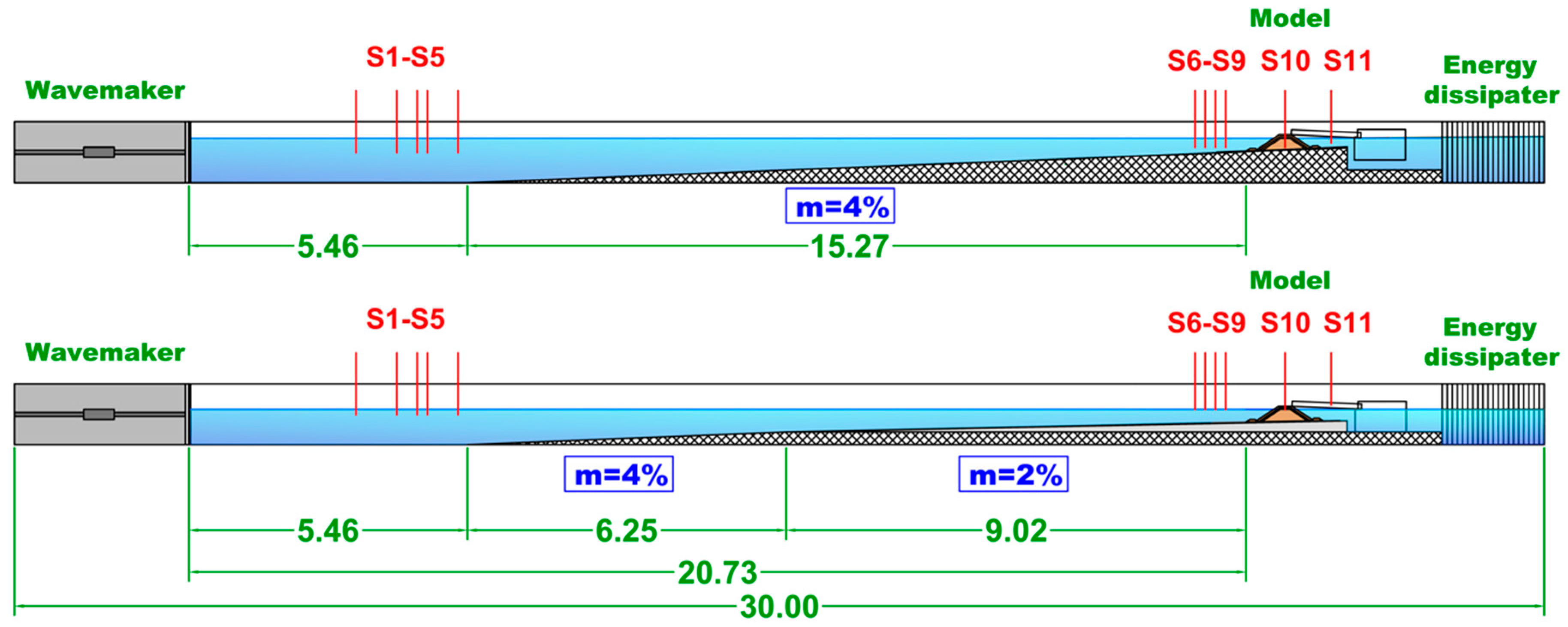
Two-dimensional small-scale physical tests were carried out in the wave flume (30 m × 1.2 m × 1.2 m) of the Laboratory of Ports and Coasts at the Universitat Politècnica de València (LPC-UPV), with a piston-type wave maker and two bottom slope (m) configurations. The first configuration corresponded to a continuous ramp of m = 4% all along the flume. The second configuration was composed by two ramps: one 6.3 m long and of which m = 4%, and one 9.0 m long and of which m = 2%. Figure 2 presents the longitudinal cross-sections of the LPC-UPV wave flume configurations as well as the location of the free surface wave gauges.

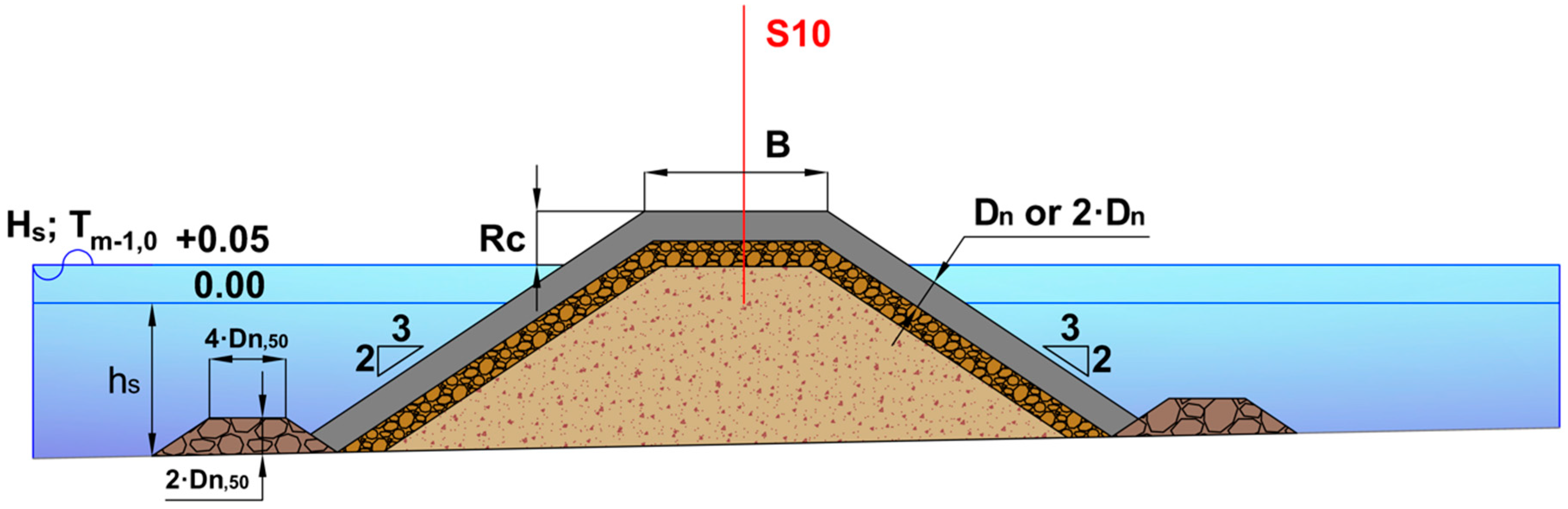
The tested cross section depicted in Figure 3 corresponds to a mound breakwater with a cotα = 1.5 slope and rock toe berms. Three armor layers were tested: a single-layer Cubipod^® armor, a double-layer randomly placed cube armor, and a double-layer rock armor. The nominal diameters or equivalent cube sizes were Dn = 3.79 cm (Cubipod^®-1L), Dn = 3.97 cm (cube-2L), and Dn = 3.18 cm (rock-2L). The rock toe berm was designed to guarantee its stability. Thus, tests in which m = 2% were performed with a medium-sized rock toe berm (Dn₅₀ = 2.6 cm), while tests in which m = 4% were conducted with a larger rock toe berm (Dn₅₀ = 3.9 cm).

Two water depths (h_s) at the toe of the structure were tested for each mound breakwater model on every foreshore configuration. In the tests for which m = 4%, h_s equaled either 20 or 25 cm. For the tests with the Cubipod^® and rock armored models, when m = 2%, h_s was either 20 or 25 cm. For the tests with the cube armored model, when m = 2%, h_s equaled either 25 or 30 cm.

For each h_s, the significant wave height (H_s = 4(m₀)^0.5) and peak period (T_p) at the wave generation zone were calculated so as to keep the Iribarren number approximately constant along the test series (Ir_p = tan α/[2 π H_s/(g T_p²)]^0.5). For each Ir_p, H_s at the generation zone (H_sg) was increased in steps of 1 cm from no damage until the armor layer failed or waves broke at the wave generation zone.

One thousand irregular waves were generated during each test following a JONSWAP spectrum (γ = 3.3). Thus, the tests lasted approximately 15 to 35 min, depending on the mean wave period. The AWACS (Active Wave Absorption Control System) system was activated to avoid multireflections. Neither low-frequency oscillations nor piling-up (wave gauge S11) were significant during the tests.

As explained in Mares-Nasarre et al. [9], two corrections were applied to the crest freeboard because of its impact on wave overtopping: (1) the extracted accumulated overtopping volumes during a working day, and (2) the natural evaporation and facility leakages. These corrections produced a small increase in the considered crest freeboard over time on the order of 10 mm for a long working day (a 3.9% variation in terms of water depth). The crest freeboard obtained after the two previous considerations is the one applied in the following analysis. A summary of the geometry and wave characteristics in the test is presented in

Table 2. Summary of geometry and wave characteristics in the LPC-UPV tests.

Armor	m [–]	Rc [m]	B [m]	hs [m]	Hs [m]	Tp [s]	Tm−1,0 [s]	# Tests
Cubipod®—1L	2%	0.07–0.12	0.24	0.20 and 0.25	0.06–0.18	1.25–2.68	1.03–2.24	53
	4%	0.07–0.12		0.20 and 0.25	0.07–0.18	1.12–2.69	1.03–2.21	49
Cube—2L	2%	0.08–0.17	0.27	0.25 and 0.30	0.06–0.18	1.00–2.68	0.91–2.25	49
	4%	0.06–0.12		0.20 and 0.25	0.09–0.17	1.25–2.69	1.17–2.33	44
Rock—2L	2%	0.10–0.15	0.26	0.20 and 0.25	0.07–0.13	1.12–2.15	0.99–1.88	21
	4%	0.10–0.15		0.20 and 0.25	0.09–0.14	1.25–2.40	1.19–2.06	19

.

A total of 11 capacitive wave gauges were located along the flume to measure the water surface elevation (see Figure 2). Wave gauges S1–S5 were placed in the wave generation zone following Mansard and Funke [16] recommendations, while wave gauges S6–S9 were placed close to the model. In order to minimize the error in the separation of incident and reflected waves, Mansard and Funke [16] proposed several criteria to calculate the distance between wave gauges as a function of the wavelength in order to separate incident and reflected waves. Nevertheless, methods in the literature to separate incident and reflected waves are not reliable in breaking conditions. Thus, in the model zone where depth-limited breaking takes place, they are not applicable. The distances from S6–S9 to the model toe were a function of the water depth at the toe of the structure, h_s. S6, S7, S8, and S9 were placed at distances 5h_s, 4h_s, 3h_s and 2h_s from the toe of the model, respectively, following the recommendations given by Herrera and Medina [17]. Wave gauge S10 was located in the middle of the model crest, and S11 was located behind the model.

The experimental set up also included three cameras to analyze the armor damage in the frontal slope, on the crest, and at the rare side of the armor using the virtual net method [18] as explained in Argente et al. [19] and Gómez-Martín et al. [20]. Overtopping discharges were collected and measured using a collection tank and a weighing system behind the model during each test.

3.1. Wave Analysis

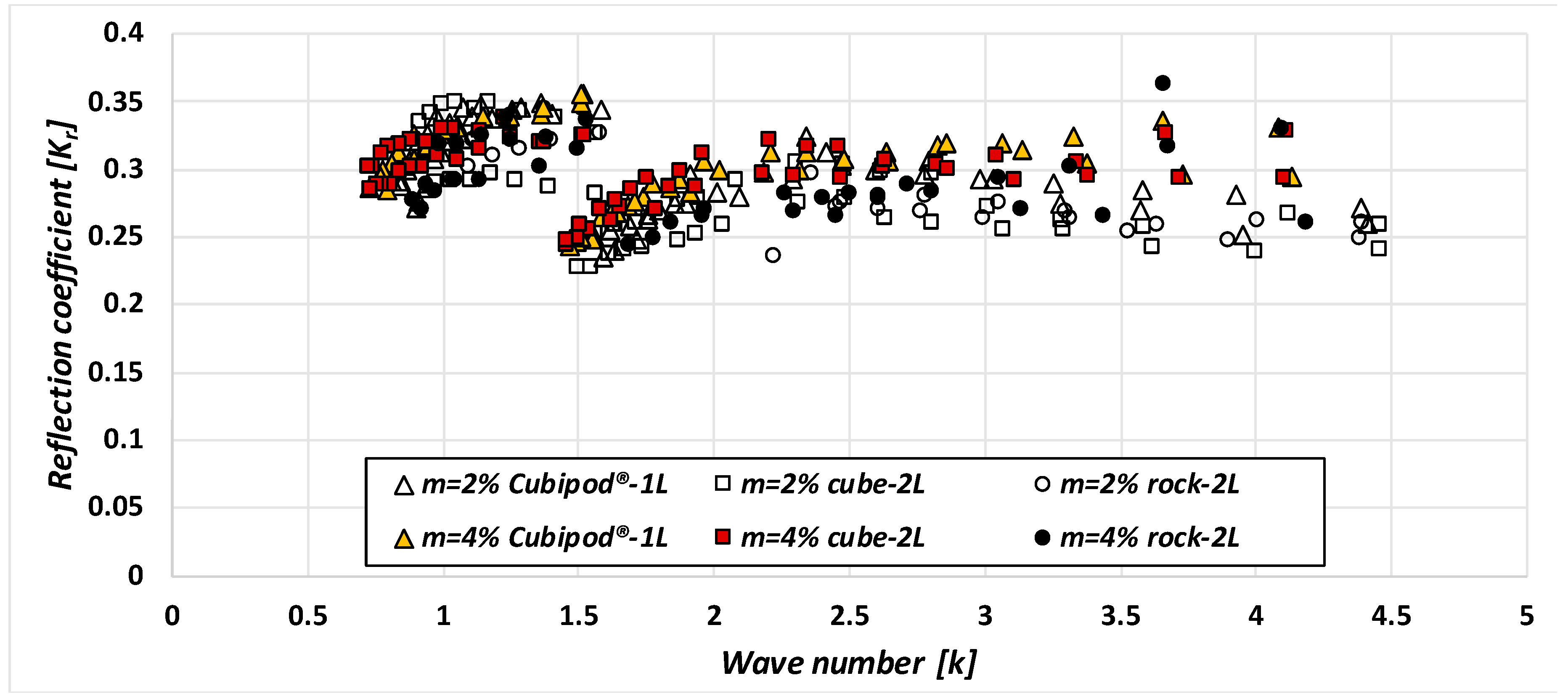
Waves were analyzed following the methodology for depth-limited breaking waves proposed by Herrera and Medina [17] and Herrera et al. [10], and similar validations to those proposed by the authors were conducted. Note that this methodology is applicable when reflection is relevant but not dominant (reflection coefficient K_r = H_s,r/H_s,i < 0.4, where H_s,r and H_s,i are the reflected and incident spectral significant wave height, respectively). Figure 4 shows the reflection coefficients measured in the wave generation zone as a function of the wave number (k = 2π/L_m0, where L_m0 is the mean deep waters wavelength, obtained from the spectral mean wave period, T₀₁ = m₀/m₁).

The LASA-V method [21] (Local Approximation using Simulated Annealing) was applied in the wave generation zone to separate incident and reflected waves using wave gauges S1–S5. Although the LASA-V method is applicable to nonlinear and nonstationary irregular waves, it is not valid for breaking waves. Thus, it is not applicable in the model zone where breaking occurs, as is the case with other existing methods in the literature. Incident waves were estimated in the model zone from the total wave gauge records, considering the reflection coefficient (K_r = H_s,r/H_s,i < 0.4, H_s,r and H_s,i being the reflected and incident spectral significant wave height, respectively) measured in the wave generation zone. Tests without a structure were conducted in this study using an efficient wave absorption assembly located at the end of the flume (K_r < 0.25 measured in the wave generation zone). Thus, the measured waves directly corresponded to the incident waves. 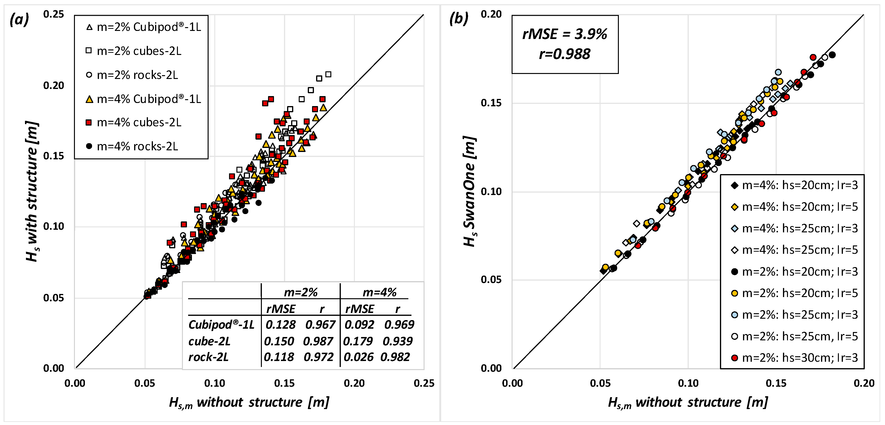Figure 5a compares the incident significant wave height in the model zone from the tests conducted with a structure (assuming the measured K_r in the generation zone as constant) and the incident significant wave height in the model zone from the tests without a structure. To quantify the goodness of fit, the relative mean squared error (rMSE) and the correlation coefficient (r) were used. The proportion of the variance not explained by the model is estimated by 0% < rMSE < 100%, whereas 0 < r < 1 assesses the correlation between the variables. Thus, the lower the rMSE is and the higher r is, the better the estimation. rMSE and r are given by Equations (1) and (2), respectively,

$$rMSE=\frac{MSE}{var}=\frac{\frac{1}{N_o}{{\displaystyle \sum }}_{i=1}^{N_o}{\left(o_i-e_i\right)}^2}{\frac{1}{N_o}{{\displaystyle \sum }}_{i=1}^{N_o}{\left(o_i-\overline{o}\right)}^2}$$

(1)

$$r=\frac{{{\displaystyle \sum }}_{i=1}^{N_o}\left(o_i-\overline{o}\right)\left(e_i-\overline{e}\right)}{\sqrt{{{\displaystyle \sum }}_{i=1}^{N_o}{\left(o_i-\overline{o}\right)}^2{{\displaystyle \sum }}_{i=1}^{N_o}{\left(e_i-\overline{e}\right)}^2}}$$

(2)

where MSE is the mean squared error, var is the variance of the observations, N_o is the number of observations, o_i is the observed value, e_i is the estimation value, $\overline{o}$ is the average of the observations, and $\overline{e}$ is the average of the estimations.

As shown in Figure 5a, a high correlation was found between the incident wave heights obtained from tests with and without a structure. Therefore, when reflection is small (K_r < 0.4), the incident significant wave height obtained from the K_r measured in the wave generation zone is a good estimator of the actual incident significant wave height. This result agrees with those reported in [10] and [17]. However, as those authors [17] pointed out, measurements without a structure are more reliable when estimating incident waves, and they were the ones used for the following analysis.

The composite Weibull distribution suggested by Battjes and Groenendijk [22] to describe the wave height distribution in shallow foreshores has been widely validated in the studies of mound breakwaters in depth-limited breaking-wave conditions (i.e., [6] or [23]). This distribution was implemented in the SwanOne software [24], which was proposed by Herrera and Medina [17] as an alternative for tests conducted without a structure. Herrera and Medina [17] applied the SwanOne model to estimate the incident wave height in the model zone by introducing the incident waves at the wave generation zone. They validated this methodology comparing the measurements in the wave flume without a structure with the results from the numerical SwanOne simulations. A similar comparison was conducted in this study and it is presented in Figure 5b. A high correlation was found between the experimental measurements and the predictions given by the SwanOne model (rMSE = 3.9%, r = 0.988). Thus, the SwanOne model is a very good estimator of the actual incident significant wave height. Since the SwanOne model provided better results than those obtained from the experimental measurements with a structure, the SwanOne predictions were used for the following analysis.

3.2. Overtopping Layer Thickness (OLT) and Overtopping Flow Velocity (OFV) Measurement

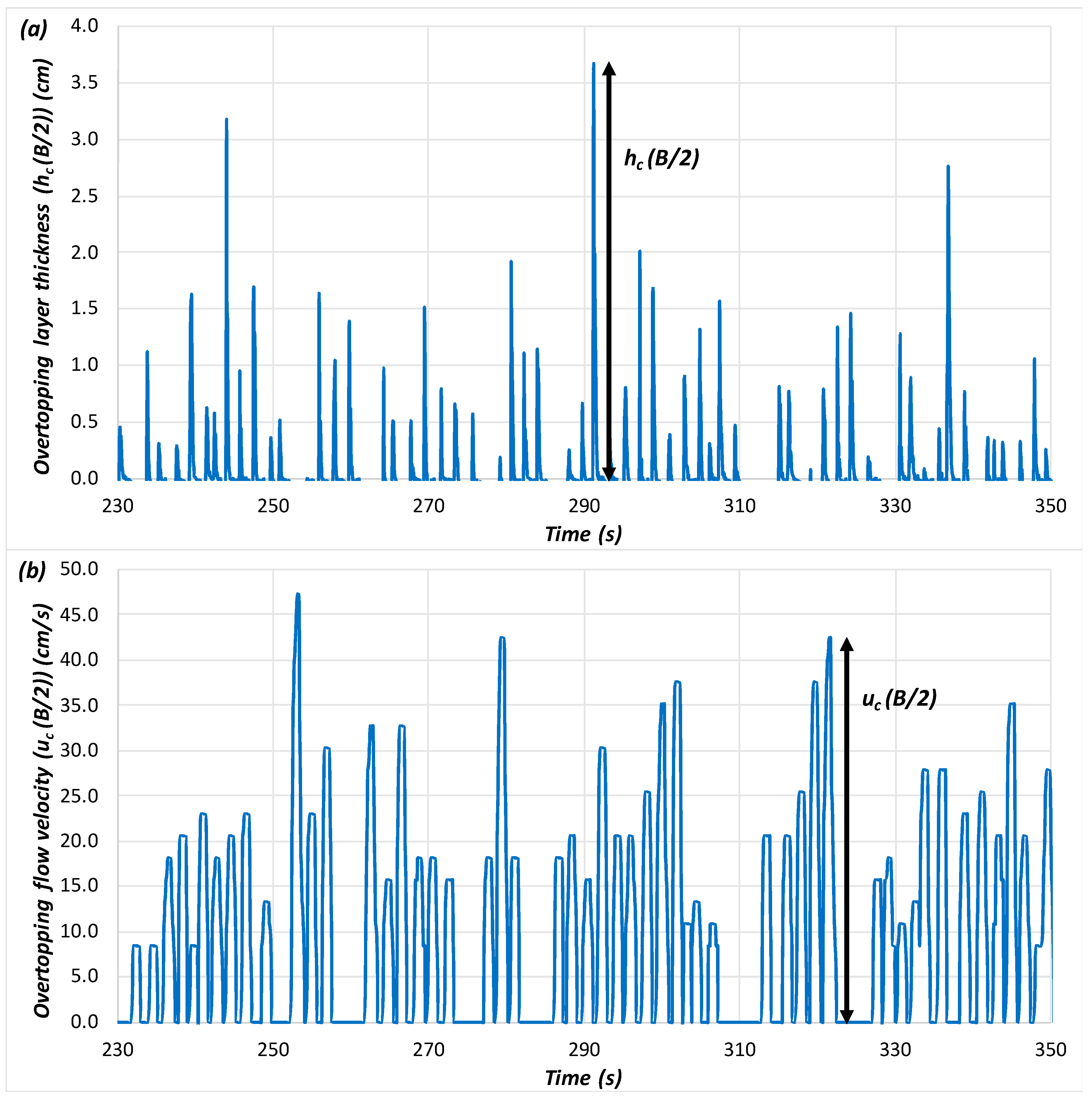
As shown in Figure 2, the capacitive wave gauge S10 was located in the middle of the breakwater crest to measure OLT. S10 was introduced into a hollow cylinder inserted in the model; S10 was filled up with water, so as to keep the capacitive wave gauge partially submerged. In order to keep the daily calibrated reference level constant, the upper part of the cylinder was closed using a lid with a slot to pass the wave gauge. The cylinder was 85 mm in diameter and 120 mm in length. Visual inspection showed a clear water surface during the overtopping events, so aeration was considered negligible. Low noise and low variation in the reference level were observed; the performance of S10 was excellent. In this study, the maximum measured OLT during each overtopping event was considered the observed h_c(B/2), as shown in Figure 6a.

The OFV was measured in 178 out of 235 physical tests using three miniature propellers on the model crest. Miniature propellers were installed in three different positions: (1) on the seaward edge of the model crest, (2) at the middle of the model crest, and (3) on the leeward edge of the crest. These miniature propellers were able to measure velocities between 0.15 and 3.00 m/s and were able to record instantaneous velocities to a frequency of 20 Hz. From the propeller recordings, the maximum values of the OFV for each overtopping event were obtained similarly to the OLT, as displayed in Figure 6b.

4. Analysis Using Neural Networks

Feedforward neural networks (NNs) are techniques from the artificial intelligence field that can be used to model nonlinear relationships between the input (explanatory) and output (response) variables. Since overtopping is a highly nonlinear problem, NNs have been applied in research and practical applications such as CLASH NN [25]. NNs have also been applied with fewer input variables and smaller datasets, with satisfactory results, to define explicit overtopping formulae [5], to assess the influence of armor placement on hydraulic stability [26], or to identify the most relevant variables to estimate forces on the crown wall [27]. Thus, when the assumption of linear relationships between variables is not valid, acceptable and reliable results may be obtained when applying NNs rather than conventional methods, such as the case of the influence of bottom slope on the overtopping layer thickness and overtopping flow velocity on mound breakwaters in depth-limited breaking-wave conditions (a highly nonlinear problem).

From the experimental data presented in Section 3, OLT exceeded by 2% of the incoming waves in the middle of the model crest, h_c,2%(B/2) and OFV exceeded by 2% of the incoming waves in the middle of the model crest, u_c,2%(B/2), were determined. Note that the velocity values out of the operational range of the miniature propellers were disregarded. As a result, 57, 30, and 80 values of u_c,2%(B/2) were considered for Cubipod^®-1L, rock-2L, and cube-2L models, respectively.

Each armor layer and overtopping variable (h_c,2%(B/2) and u_c,2%(B/2)) was studied independently, so the analyses described in the following paragraphs are repeated three times (Cubipod^®-1L, rock-2L, and cube-2L) for each overtopping variable (h_c,2%(B/2) and u_c,2%(B/2)). The three armor units were studied independently to keep the model as simple as possible. The diagram of this analysis is illustrated in Figure 7.

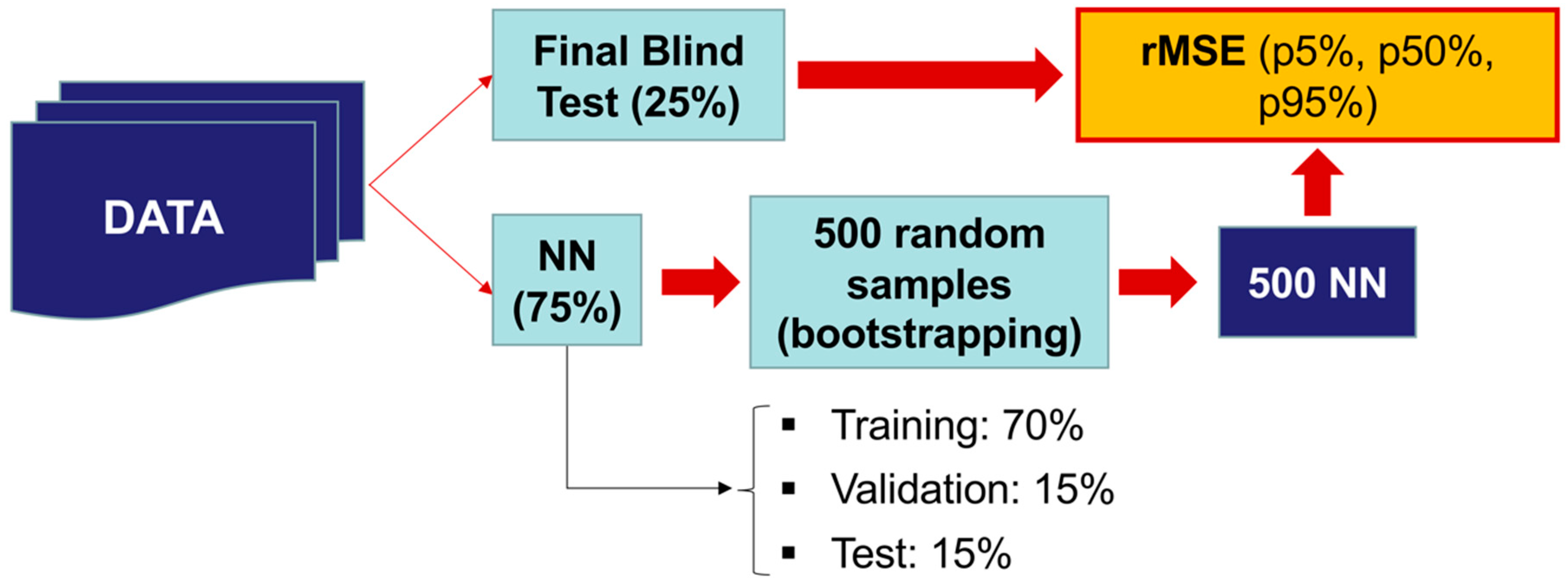
Initially, the data of each armor were divided in two sections: 25% of the data was kept for a final blind test (FBT), and 75% of the data was used for the NN training (T). The bootstrapping technique is applied to the 75% of the data for training to generate 500 random datasets. This technique consists of the random selection of N data from N original datasets with a probability of each datum to be selected each time of 1/N. Thus, some data were absent in a resample, whereas some data were chosen once or more than once. The 500 random datasets were used to train 500 NNs. The goodness of fit of these NNs was evaluated using FBT data with rMSE. The average value of rMSE and its variability is obtained.

Multi-layer feed-forward NNs with only one hidden layer were used, and a hyperbolic tangent sigmoid transfer function was applied. The NN structure was composed of one input layer of four neurons (N_i), one hidden layer of three neurons (N_h), and one output layer of one neuron (N_o). The number of free parameters of the NN model is given by P = N_o + N_h (N_i + N_o + 1) = 19. Overlearning is likely to occur when P/T ≥ 1, when P/T = 0.63 in the worst case. Additionally, an early stopping criterion was applied to prevent overlearning (see MATLAB^® [28]), dividing the 75% dataset used for training (T) into three sections: training (75% × 70%), validation (75% × 15%), and test (75% × 15%). Data in the training section were used to formally train the NN, updating the biases and weights. Data in the validation section were used to monitor the error after each training step and to stop the training when the error on this subset starts growing (an indication of overlearning). Data in the test section were not used during the training process, but to compare different models as a cross validation. As previously mentioned, every armor layer was studied independently to maintain the simplest NN; in the case of including the three armor layers in one NN, one or several extra input neurons would be needed (e.g., armor element, number of armor layers). In addition, to guarantee a proper NN training, a balance dataset is needed, so the same number of tests from each armor layer should be used. Therefore, the number of tests used should be limited to the number of cases of the smallest dataset. In other words, only 40 tests would be used (rock-2L), even if 102 and 93 cases are available for Cubipod^®-1L and cube-2L, respectively.

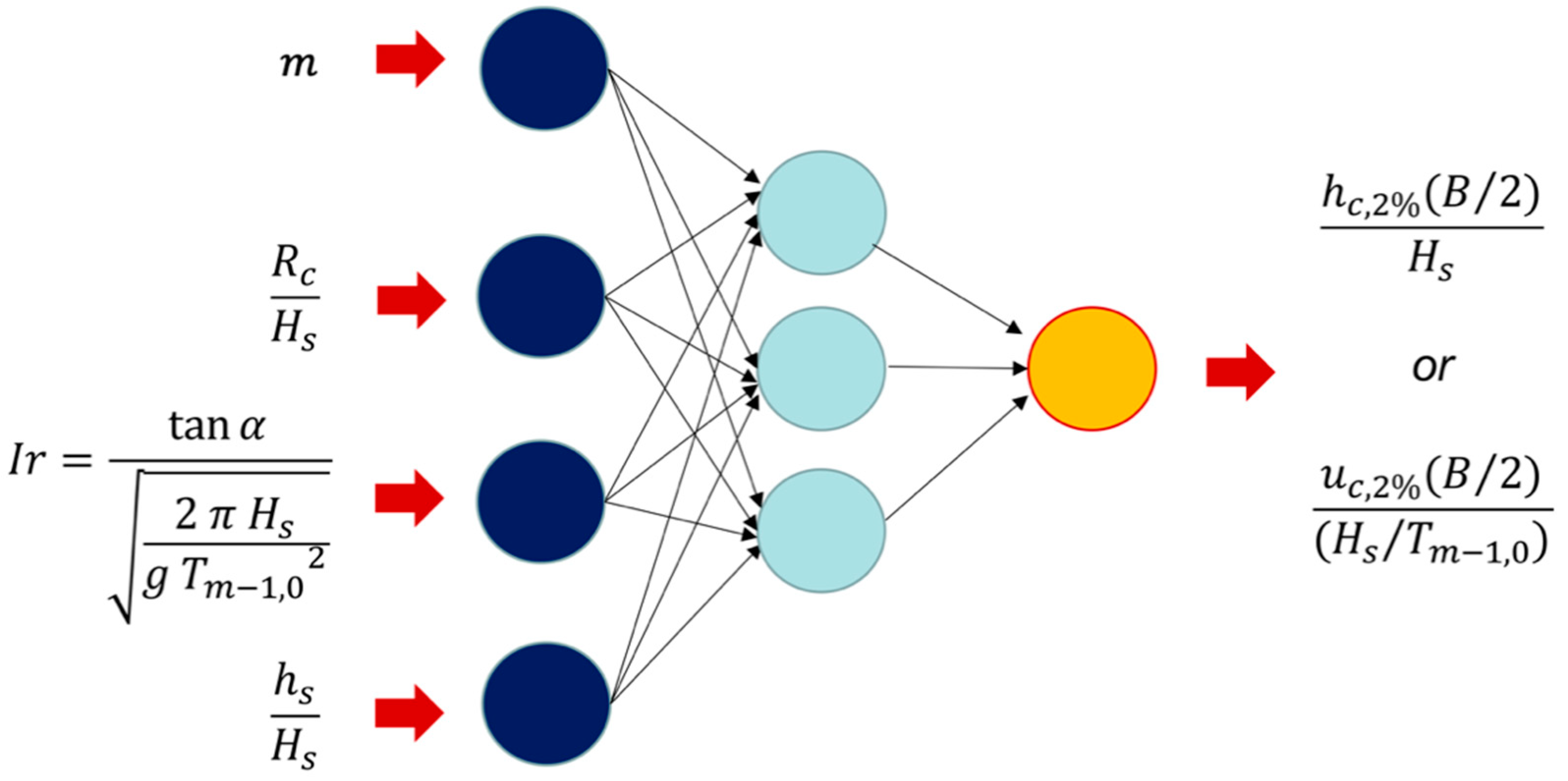
As shown in Figure 8, both h_c,2%(B/2) and u_c,2%(B/2) were analyzed as dimensionless variables (h_c,2%(B/2)/H_s and u_c,2%(B/2)/(H_s/T_m−1,0)). Five input variables were considered as significant to describe OLT and OFV: the significant wave height (H_s), the spectral period (T_m−1,0), the crest freeboard (R_c), the water depth at the toe of the structure (h_s), and the bottom slope (m). Nevertheless, only four dimensionless variables were considered to feed the NN model (see Figure 8): m, R_c/H_s, Ir = tanα/(2πH_s/g/T_m−1,0²) and h_s/H_s.

4.1. Optimum Point to Estimate Wave Parameters

The method shown in Figure 7 is repeated seven times for each armor layer and overtopping variable (7 × 3 × 2 = 42 times), modifying the incident wave height (H_s) given to feed the model. The considered H_s values were H_s estimated at the toe of the structure, H_s estimated at a distance of h_s from the toe of the model, H_s at 2h_s from the toe of the model, as so on until 6h_s from the breakwater toe.

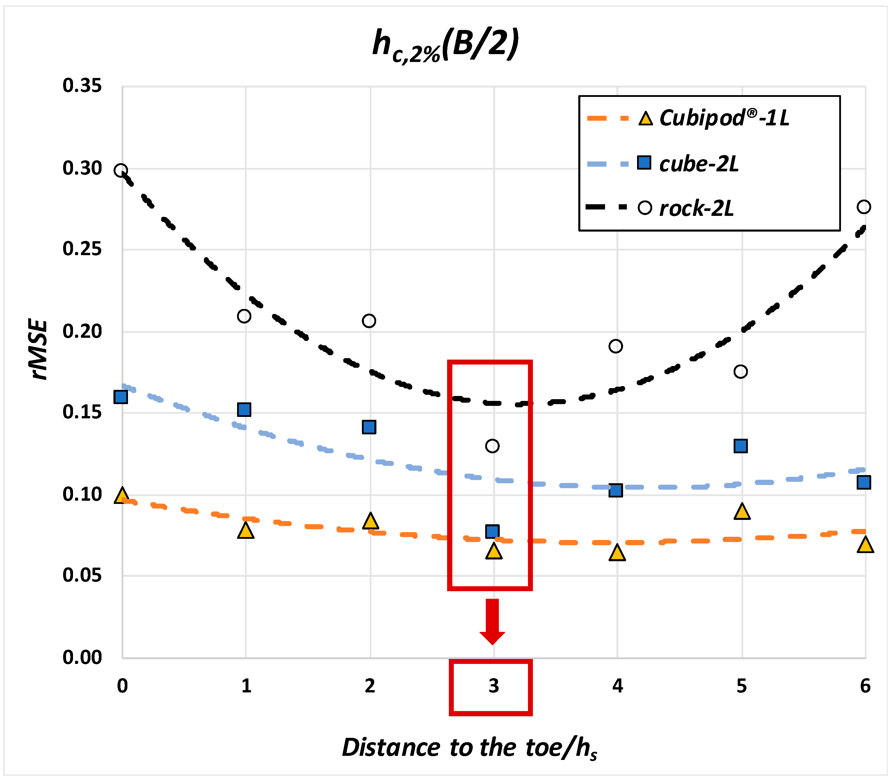
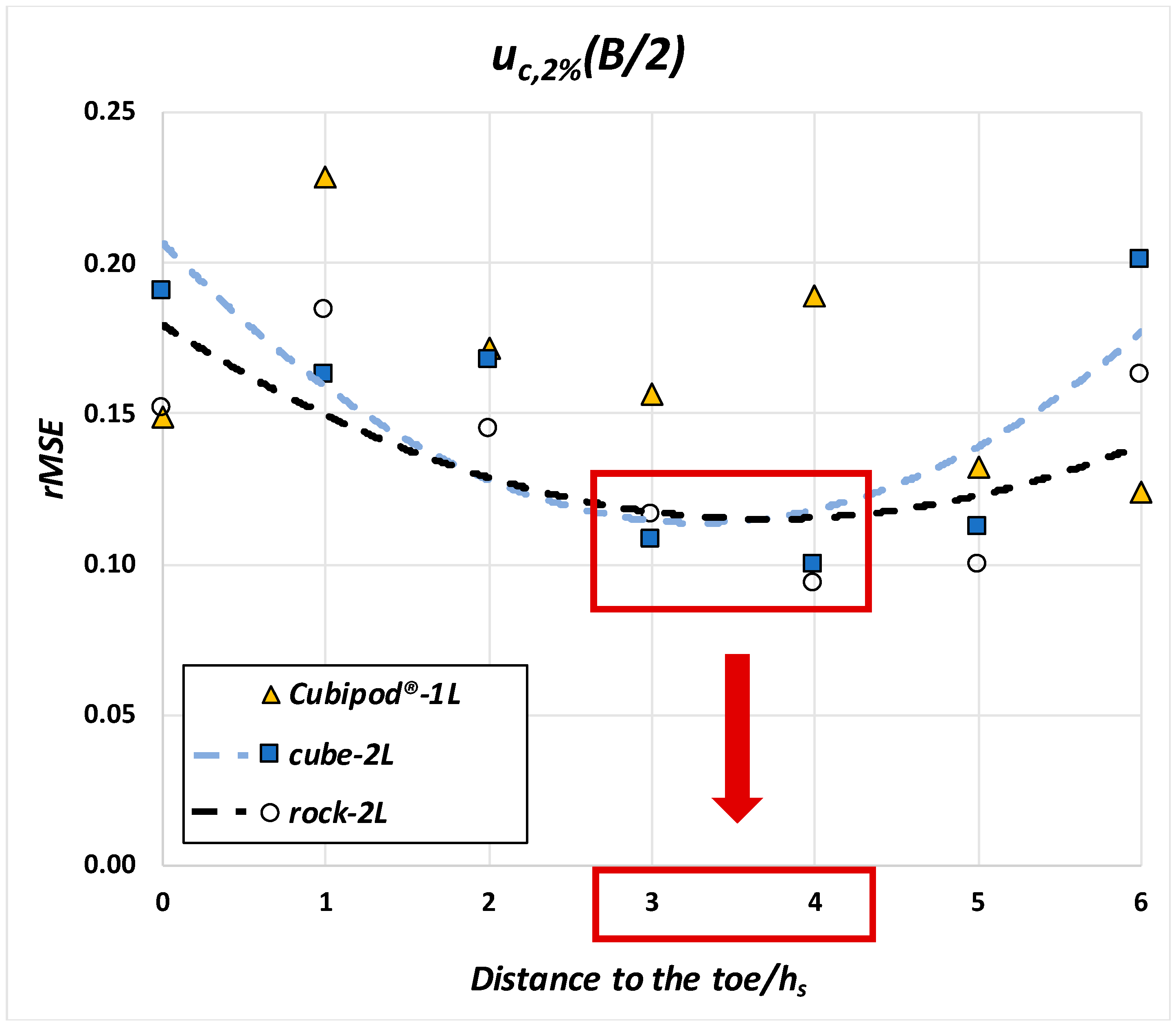
As a result, the evolution of the percentiles of rMSE can be obtained as a function of the distance from the model toe where H_s is calculated. Percentiles 5%, 50%, and 95% were used to characterize rMSE. Figure 9 presents the rMSE of the NN p50% for h_c,2%(B/2) while Figure 10 shows the results for u_c,2%(B/2). Here, the x-axis represents the distance from the toe to the structure to the point where H_s is calculated as a multiple of h_s, whereas the y-axis presents the median rMSE (p50% NN).

The lowest rMSE for h_c,2%(B/2) for the three armor layers was obtained around the zone of H_s estimated at a distance of 3h_s from the breakwater toe, as shown in Figure 9. In the case of u_c,2%(B/2), no clear tendency was identified for the Cubipod^®-1L armor. This may be due to the low number of values for the 2% bottom slope (N = 13 for m = 2%, and N = 44 for m = 4%). For rock-2L and cube-2L armors, the optimum point to estimate H_s was located between 3h_s and 4h_s from the toe of the model (see Figure 10). Thus, a distance of 3h_s from the model toe was selected as the optimum zone to estimate H_s for the calculation of h_c,2%(B/2) and u_c,2%(B/2). This point was also selected by Herrera et al. [10] to better describe the hydraulic stability of rock-armored rubble mound breakwaters in depth-limited wave conditions. This distance approximately corresponds to the distance of 5H_s proposed by Goda [29] and recommended by Melby [30] to determine wave parameters, when considering H_s in breaking wave conditions for vertical breakwaters.

4.2. Influence of the Bottom Slope on OLT and OFV

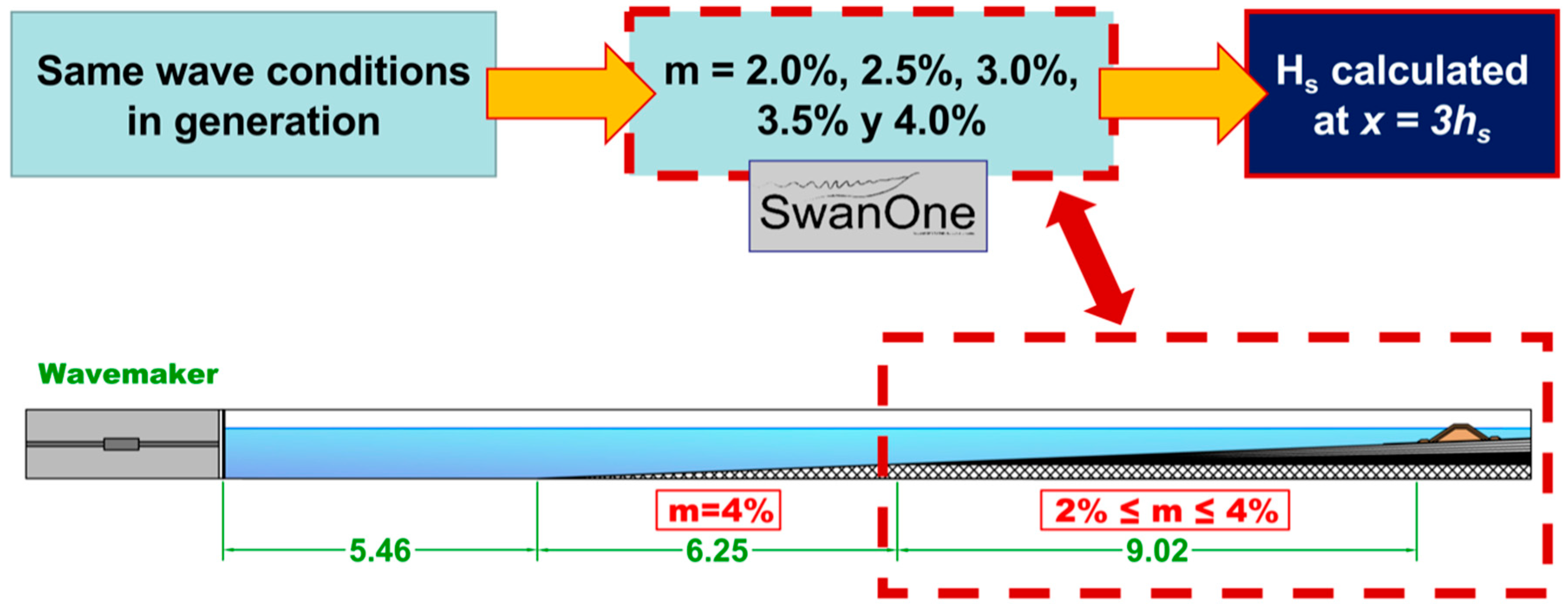
In the previous section, the optimum zone to estimate H_s for the calculation of h_c,2%(B/2) and u_c,2%(B/2) was identified at a distance of 3h_s from the model toe. Here, the influence of bottom slope on h_c,2%(B/2) and u_c,2%(B/2) is assessed. To this end, wave conditions were considered in the wave generation zone (H_s,g and Ir_g), and they were propagated along the wave flume using the SwanOne model [24] up to a distance of 3h_s from the structure toe. Five numerical flumes (see Figure 11) were considered in this propagation, and the gradient of their bottom slope varied within the tested range (m = 2.0%, 2.5%, 3.0%, 3.5%, and 4.0%).

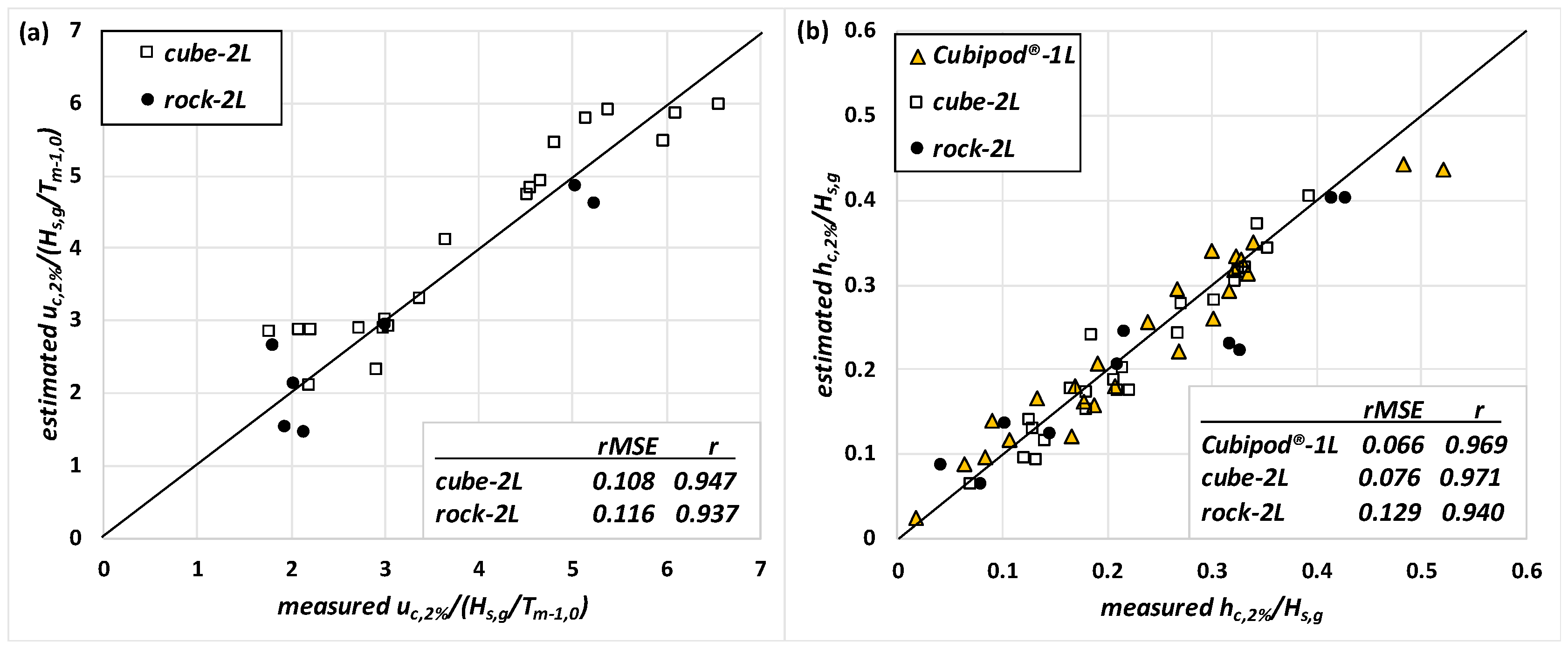
Using the wave characteristics obtained from the propagation, simulations were conducted using NN p50%. Thus, h_c,2%(B/2) and u_c,2%(B/2) were obtained for five different bottom slopes and the same wave conditions in the wave generation zone. Figure 12 shows the cross-validation of NNs p50% with the final blind test data. The agreement between p50% NNs and the final blind-test data was very good (0.937 ≤ r ≤ 0.971; 0.066 ≤ rMSE ≤ 0.129).

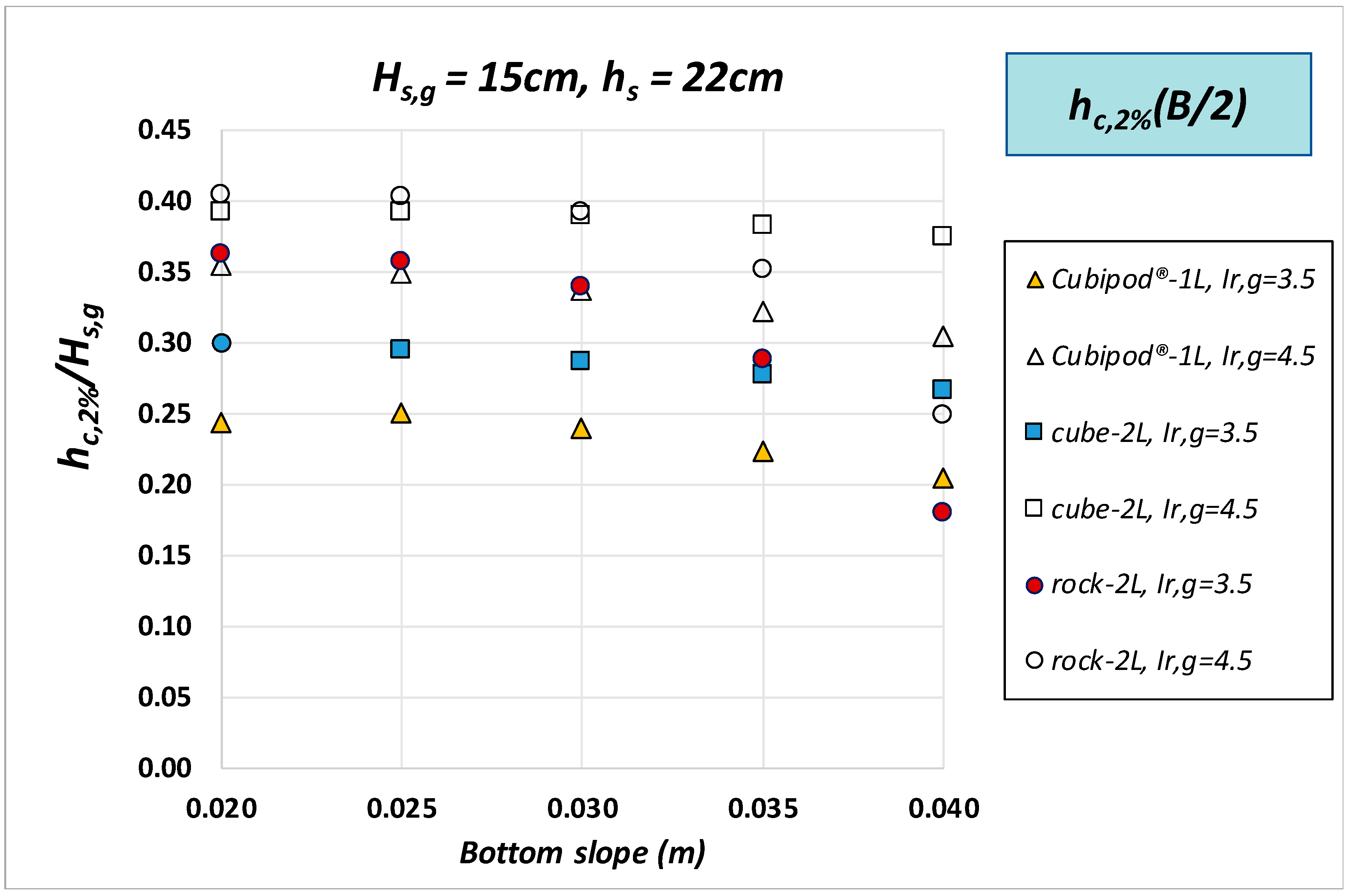
Figure 13 illustrates the evolution of h_c,2%(B/2) as a function of m for different wave conditions and the three armor layers (Cubipod^®-1L, cube-2L, and rock-2L). h_c,2%(B/2) decreased for increasing values of m.

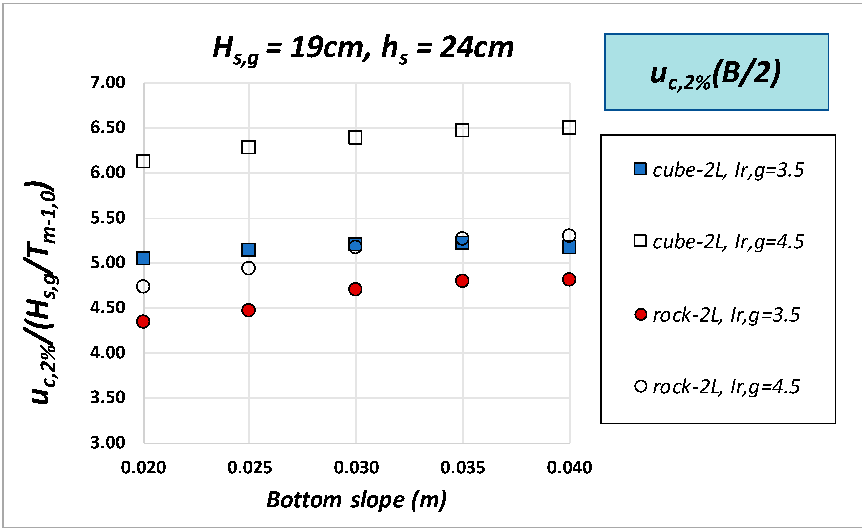
Figure 14 shows the progression of u_c,2%(B/2) for cube and rock armors when varying m for different wave conditions and two of the three studied armor layers. u_c,2%(B/2) slightly increased with increasing values of m.

5. Conclusions

Overtopping is an increasing risk on coastal structures because of the rising sea levels caused by climate change and social demands to reduce the visual impacts. The safety of pedestrians is a relevant issue during recreational activities on the breakwater crest (e.g., fishing and photography). In order to assess pedestrians’ risk, the overtopping layer thickness (OLT) and the overtopping flow velocity (OFV) have been proposed as significant variables.

Few studies are focused on OLT and OFV estimation on coastal structures. These studies only considered variables related to geometry and wave conditions for OLT and OFV calculation. However, most of the mound breakwaters are built in the surf zone, and the bottom slope is an important factor in depth-limited breaking-wave conditions.

In this study, 235 2D physical tests were conducted at the LPC-UPV wave flume with two bottom slopes (m = 2% and m = 4%) and models of mound breakwaters with a single-layer Cubipod^® armor, a double-layer rock armor, and a double-layer randomly placed cube armor. A total of 178 tests measured both OLT and OFV, while an additional 57 tests only measured OLT. OLT was measured using a capacitance wave gauge, while OFV was measured using miniature propellers.

Using neural networks (NNs) and bootstrapping techniques, the optimum point to estimate the significant wave height (H_s) to calculate the OLT exceeded by 2% of incoming waves (h_c,2%(B/2)) and the OFV exceeded by 2% of incoming waves (u_c,2%(B/2)) was studied for each armor. A distance of 3h_s from the breakwater toe was determined as the optimum zone to estimate H_s for the calculation of h_c,2%(B/2) and u_c,2%(B/2).

In order to analyze the influence of m on h_c,2%(B/2) and u_c,2%(B/2), fixed wave conditions in the wave generation zone were propagated along five numerical wave flumes with different bottom slopes (m = 2.0%, 2.5%, 3.0%, 3.5%, and 4.0%) using the SwanOne software [24] up to a distance of 3h_s from the model toe. Using the median rMSE NNs (p50% NN), it is observed how h_c,2%(B/2) decreases and u_c,2%(B/2) slightly increases as the gradient of the bottom slope increases.