Bulk Wave Dissipation in the Armor Layer of Slope Rock and Cube Armored Breakwaters

Abstract

The objective of this research is to analyze the interaction of the incident wave train with a mound breakwater (specifically, dissipation in the armor layer) and to quantify the performance of the structure built with different types and sizes of armor units. The generalized $\mathsf{\Pi }$-Buckingham theorem is invoked to choose a complete set of independent variables that govern the principal interaction processes. The analysis is based on two sets of experimental data obtained in the wave flume of IISTA, University of Granada, and in the wave flume of Aalborg University. The bulk dissipation depends on the product of the relative water depth and the incident wave steepness, $(h/L)(H_I/L)$, the relative size of the armor diameter, $D_a/H_I$, the relative thickness, $e/L$, the shape and specific placement criterion, the characteristics of the porous core, $B^{*}/L$, $D_{50,p}/L$, and the slope angle of the breakwater. For a given breakwater, the product of $(h/L)(H_I/L)$ can be used to identify and quantify three hydrodynamic performance regimes: reflective, dissipative and transitional, based on the prevalent interaction processes. Moreover, the dimensional analysis provides a functional relationship between the stability parameter and the bulk dissipation. For two mound breakwaters, one built with cubes of $D_a=49.6$ mm and the other one with rocks of $D_a=44.0$ mm, the bulk dissipation is almost similar over the entire range of $(h/L)(H_I/L)$. These results could be useful for the assimilation of data obtained in different wave flumes, the optimization of the breakwater design and to revise the notional permeability parameter.

1. Introduction

The main function of breakwaters is to protect harbors and coastal structures from wave action. Mound breakwater is the most frequent typology due to its main function to break/dissipate incident wave and its possibility to be constructed using different types and sizes of armor pieces. Its hydrodynamic performance depends on the wave kinematic and dynamic regimes and the incoming wave energy transformation while interacting with the breakwater section [1,2].

The energy dissipation of a wave train on a breakwater slope is mainly caused by the transport of turbulence during the following processes: (i) wave evolution and, eventually, wave-breaking on the free surface of the slope; (ii) circulation and friction with the main armor layer; and (iii) wave propagation through the secondary layers and porous core. Simultaneously, part of the incident energy is reflected by the changes in the characteristics of the breakwater during its propagation through the slope, main armor layer, secondary layer and porous core, impinging the crown, and while propagating landward of the breakwater section [3].

In the last two decades, numerical predictions of the wave-breaking on a smooth and impermeable slope have been published using different numerical techniques [4,5,6,7,8,9]. These results provide detailed information on the transport of turbulent kinetic energy due to the interaction process of the wave train with the slope. On the other hand, the propagation of a wave train (regular or irregular) through a rectangular porous medium is widely analyzed, both theoretically and experimentally. It is concluded that the Forchheimer equation quantifies (reasonably well) the bulk resistance (or the momentum consumption) in the porous medium [10,11,12]. Moreover, for applied maritime engineering the equivalent hypothesis of Lorentz provides satisfactory results of the wave energy dissipation [13,14].

Unfortunately, reflection and dissipation during shoaling and the eventual breaking of the wave on a slope with a permeable core do not have a theoretical model equivalent to the Forchheimer equation, and most studies are based on numerical [15,16,17,18,19,20,21] and physical experimentation [11,13,14,22,23,24]. All of them confirmed that the dimensions of the main armor layer and the unit type significantly affect the values of the reflected energy coefficient, $K_R^2$, and the bulk dissipation rate, $D^{*}$, as well as the run-up, $R_u$, run-down, $R_d$, and, where appropriate, the overflow rate, $Q_c$ on overtoppable structures [25].

In the practical maritime engineering, wave reflection and transmission of the wave train impinging a breakwater are determined by applying semi-empirical formulas. Most of them developed under the assumption of the Iribarren number [26] as the main independent variable. In addition, its application is based on the correspondence between the value of $I_r$ and the type of wave-breaking on the slope [27,28,29]. The number of Iribarren is defined by a characteristic wave height and length of the incident wave train, H and L, respectively, and the slope angle, $\alpha$: $I_r=tan\left(\alpha \right)/\sqrt{H/L}$.

This semi-empirical approach led to a qualitative and quantitative step in the calculation skills of mound breakwaters. However, over the years, the experimental dispersion of the data promoted both the identification of the sources of uncertainty and the re-analysis of such formulas. In the context of the present work (wave energy dissipation), two proposals are remarkable: the notional permeability, P [30], and/or the partial coefficients $\gamma$, to “quantify” the dependence of the results on the permeability and the geometric configuration and type of armor of the main armor layer and the characteristics of the core [31,32]. Intriguingly, P and the coefficients $\gamma$, depend again on the Iribarren number. One of the consequences to proceed in that way is the difficulty to evaluate the uncertainty of the engineering design, effecting its optimization [2,33].

In this regard, Vílchez et al. [24] analyzed the hydraulic performance of frequently built breakwater typologies and showed that the averaged transformation of the wave inside the porous medium depends on the scattering parameter, $A_{eq}/L^2$ (being $A_{eq}\approx B^{*}h/L$ the area of the porous core under the still water level, $B^{*}$ is a characteristic width of the core and h, the water depth), and the relative core grain size, $D_{50,p}/L$. Next, Clavero et al. [34] modified the Iribarren number by replacing $tan\left(\alpha \right)$ with the the scattering parameter. Its application improves significantly the quantification of the reflection coefficient, $K_R^2$, in the transition and the reflection-dominated regions. Note that usually the breakwater stability worsen in the transition region [35,36].

Nevertheless, this representation does not allow to identify the most likely breaker types and water surface evolution in each region, specifically in the dissipation-dominated and transition regions, and their relationships with the bulk dissipation in the breakwater. To consider those aspects, Díaz-Carrasco et al. [37] reworked the dimensional analysis done by Battjes [29], and showed that the wave breaking type and the dissipation process on a impermeable plain steep slope depends on, both, the relative water, $h/L$, and the incident wave steepness, $H_I/L$, computed at the toe of the slope. Then, they completed the types of breaking, differentiating weak and strong bore or collapsing [6], and weak and strong plunging [9,38]. For permeable slopes, the dissipation in the main and secondary layers and the core also play a role. Thus, in addition to $h/L$ and $H_I/L$, wave energy transformation and breaker types depend on $D_{50,p}/L$, $B^{*}/L$, $D_a$, e, for each slope angle; where $D_a$ and e are the equivalent (or nominal) diameter of the amour unit and the main layer thickness respectively. When these results were compared with those for an impermeable slope with the same angle, significant changes were identified.

Consequently, the main objective of this research is to analyze the dissipation process due to the interaction of the incident wave train with the main armor layer, and to quantify the performance between mound breakwaters built with different types and sizes of armor units. For that, two sets of experimental data were used (obtained in the wave flume of Aalborg University and in the wave flume of IISTA-University of Granada (UGR)). The latter are the experimental data presented in Clavero et al. [34]. A generalized $\mathsf{\Pi }$-Buckingham theorem is applied [39] which helps to reduce the number of independent similarity parameters. Dimensional analysis provides a truly complete identification of the independent variables that specify the bulk dissipation and its components. Moreover, it yields a relationship between the bulk dissipation and the stability number.

This paper is organized as follows: Section 2 presents the problem formulation, which includes the dimensional analysis and the working hypotheses considered in this study. Section 3 outlines the physical experimental setups performed in IISTA-University of Granada and in Aalborg University. Section 4 presents and analyzes the experimental space, the results and the most likely breaker types observed, and then, the relative bulk dissipation in the main armor layer depending on the type and size of the unit piece is presented. Section 5 and Section 6 gather the discussion of the results and the conclusions derived from this research, respectively.

2. Problem Formulation

The main objective of this research is to experimentally analyze the dissipation process due to the interaction of an incident wave train and a mound breakwater. This work is devoted to characterize the dependence of the bulk dissipation on the characteristics of the main armor layer. The bulk dissipation is not an observed variable but, determined by solving the wave energy conservation equation in a fixed and finite control volume that contains the breakwater section,

$$F_I-F_R-F_T-D^{{}^{\prime }*}=0$$

(1)

where $F_i=C_{g,i}{E}_i$; $i=I$, R, T represents the mean energy flux of the incident, reflected and transmitted wave trains, respectively; $E_i=(1/8)\rho g{H}_i^2$ represents the wave energy; $H_i$ is the wave height; $\rho$ is the water density and g is the gravity acceleration; and $C_{g,i}=f(h,L)$ is the linear theory group celerity of the energy propagation. $D^{{}^{\prime }*}$ is the bulk dissipation in the control volume. If water depth is constant, Equation (1) can be written as follow,

$$D^{*}=1-\left[K_R^2+K_T^2\right]$$

(2)

where $K_R^2$, $K_T^2$, are the module of the reflection and transmission coefficient, respectively, and $D^{*}$ is the total bulk dissipation per unit of wave incident energy. The bulk dissipation can be split in three main contributions to the transport of turbulence: (i) $d_1^{*}$, wave evolution and eventually wave-breaking on the free surface of the slope; (ii) $d_2^{*}$, circulation and friction with the main armor layer; and (iii) $d_3^{*}$, wave propagation through the secondary layers and porous core, thus,

$$D^{*}=d_1^{*}+d_2^{*}+d_3^{*}+\delta$$

(3)

where $\delta$ is the error independent of the dissipation processes. Not quantified uncertainty is assumed to be compressed in $\delta$.

Developing a dimensional analysis by means of Buckingham’s $\mathsf{\Pi }$-theorem (see Appendix A), bulk dissipation can be expressed as a function of the following dimensionless variables:

$$D^{*}={\mathsf{\Psi }}_D\left[\left(\frac{H_I}{L},R_{e,D_a},N_s\right);\left(\frac{h}{L},\frac{D_{50,p}}{L},\frac{B^{*}}{L},\frac{e}{L}\right)\right]$$

(4)

Regarding Equation (3), the bulk dissipation can by split in three component $(d_1^{*},d_2^{*},d_3^{*})$ quantifying the contribution due to wave evolution on the slope, the interacting flow within the armor layer and wave propagating through the secondary layers, core and, eventually transmitting landward. Following Díaz-Carrasco et al. [37], then

$$d_1^{*}={\mathsf{\Psi }}_D\left[\frac{h}{L},\frac{H_I}{L}\right]$$

$$d_2^{*}={\mathsf{\Psi }}_D\left[\left(N_s,R_{e,D_a},\frac{e}{L}\right);\left(\frac{h}{L},\frac{H_I}{L}\right)\right]$$

(5)

$$d_3^{*}={\mathsf{\Psi }}_D\left[\left(\frac{D_{50,p}}{L},\frac{B^{*}}{L}\right);\left(\frac{h}{L},\frac{H_I}{L},N_s\right)\right]$$

Notice that, generally speaking, $e/L\approx n_l{D}_a$, depending on the number of units placed per unit area.

In the present research, the following hypothesis is adopted: “If the armor layer of two mound breakwaters are built with the same armor unit but, (1) with different size, or (2) with different thickness, or placement criterion, then the differences between their respective bulk dissipation are mainly due to the variation in $d_2^{*}$

$${\left(D^{*}\right)}_{ma1}-{\left(D^{*}\right)}_{ma2}\approx {\left(d_2^{*}\right)}_{ma1}-{\left(d_2^{*}\right)}_{ma2}+\mathrm{error}$$

(6)

where the subscripts $ma1$ and $ma2$ identify two breakwaters being compared.”

3. Experimental Methodology

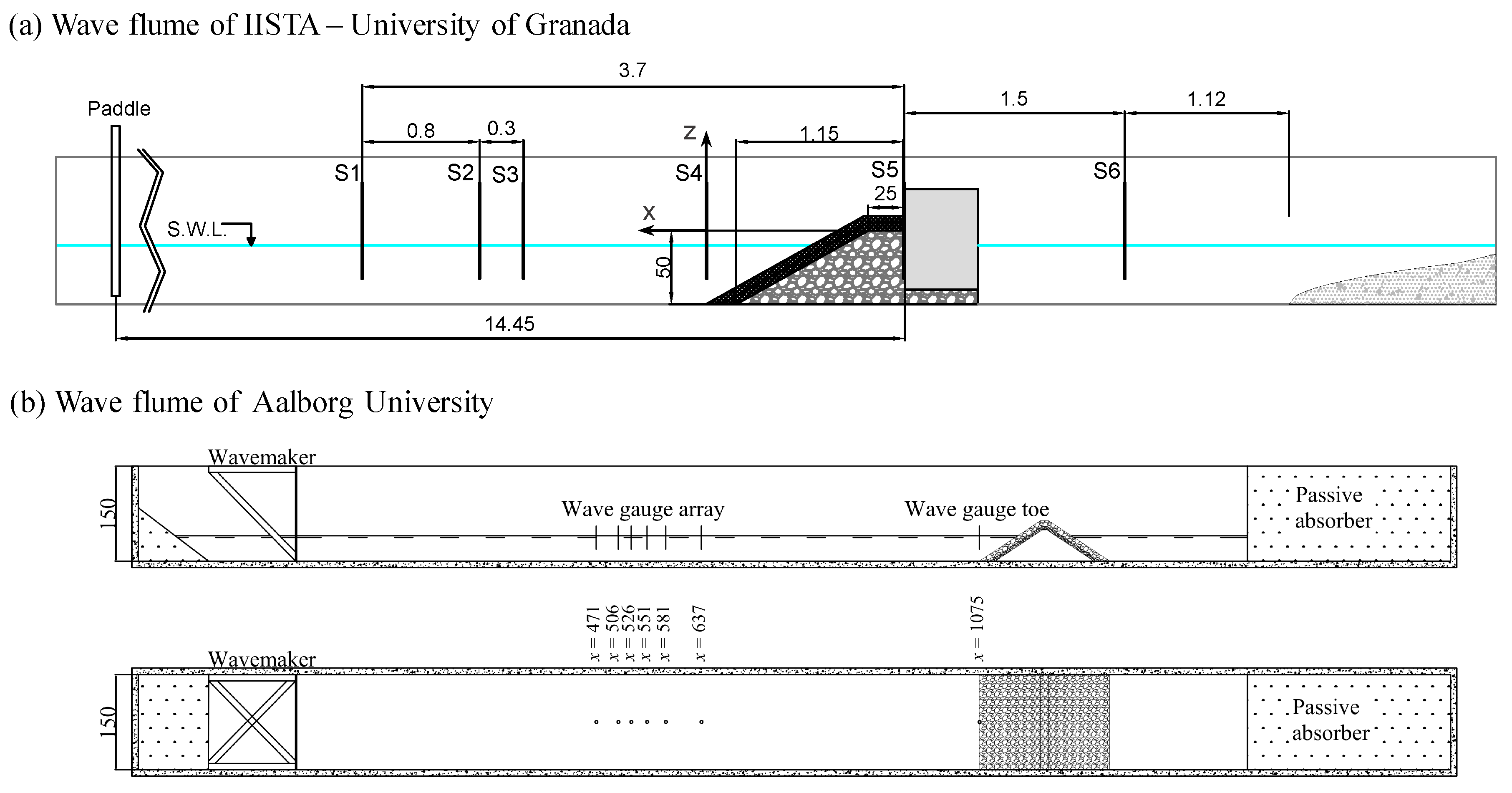
3.1. Experimental Setup

Two sets of experimental data were collected in two different laboratories. The first dataset were performed in the wave-current flume of IISTA, University of Granada (IISTA-UGR). The model consisted on a rubble-mound breakwater with crown wall composed of a double armor layer of cubes and a permeable core of fine gravel. The second set of experimental data was obtained from laboratory tests done in the wave flume of Aalborg University (AAU) [40]. The physical model tested was a conventional double armor layer mound breakwater with two different armor units, rocks and cubes, with a porous core built with fine gravel. Figure 1 shows the scheme of both wave flumes of IISTA-UGR (a) and AAU (b), while Figure 2 shows a sketch of the physical model tested at IISTA-UGR (a) and at AAU (b).

Geometrical parameters of the physical models for both laboratories are summarized in

Table 1. Geometric parameters of (A) the rubble mound breakwater with crown wall tested in the laboratory of IISTA-UGR, and (B) the conventional rubble mound breakwater tested in the laboratory of Aalborg University. $B_b$ is the width of the top of the breakwater; $F_{MT}$ is the height of the porous core; $D_{eq}$ is the equivalent diameter of the main armor layer, where the cube volume is equated to the volume of a sphere; $\alpha$ and $\beta$ are the seaward and landward slopes of the breakwater, respectively; ${\rho }_{s,a}$ and ${\rho }_{s,p}$ are the densities of the armor units and core, respectively; $F_c$ is the free-board; B is the width of the caisson; $h_b$ is the caisson foundation depth; $n_p$ is the porosity of the core according to CIRIA et al. [41]; and $D_{50,f}$ is the diameter of the filter. The values of core porosity, $n_p$, and densities, ${\rho }_{s,a}$, ${\rho }_{s,p}$, for the conventional rubble mound breakwater were provided by Aalborg University.

(A) Breakwater model of IISTA-UGR
Armor unit cubes size (mm)	$D_a=D_{eq}$ (mm)	$B_b$ (m)	${\rho }_{s,a}$ (t/m${}^3$)	$F_c$ (m)	$h_b$ (m)	$cot\left(\alpha \right)$	B (m)	$F_{MT}$ (m)	$D_{50,p}$ (mm)	${\rho }_{s,p}$ (t/m${}^3$)	$n_p$
l = 25 mm	31. 0	0.25	2.07	0.25	0.10	1.5	0.5	0.55	12	2.83	0.391
l = 33 mm	40.9		2.18
l = 38 mm	47.1		2.2
l = 44 mm	54.6		2.21
l = 65 mm	80.6		2.27
(B) Breakwater model of Aalborg University
Armor unit	$D_a=D_{eq}$ (mm)	$B_b$ (m)	${\rho }_{s,a}$ (t/m${}^3$)	Filter $D_{50,f}$ (mm)	$cot\left(\alpha \right)$	$cot\left(\beta \right)$	$F_{MT}$ (m)	$D_{50,p}$ (mm)	${\rho }_{s,p}$ (t/m${}^3$)	$n_p$
Cubes l = 40 mm	49.6	$3D_a$	2.30	15	1.5	1.5	0.55	5.8	2.80	0.37
Rocks	44 0	$3D_a$	2.62	15	1.5	1.5	0.55	5.8	2.80	0.37

. Wave conditions tested in both laboratories can be seen in

Table 2. Wave conditions tested in (A) the laboratory of IISTA-UGR, and (B) the laboratory of Aalborg University. Target parameters for irregular waves generated with a Jonswap spectrum.

(A) Wave conditions of IISTA-UGR
Armor unit cubes size (mm)	$T_{p,target}$ (s)	$H_{m0,target}$ (m)
l = 25 mm	[1.05–3]	[0.04–0.08]
l = 33 mm	[1.05–3]	[0.04–0.10]
l = 38 mm	[1.05–3]	[0.04–0.10]
l = 44 mm	[1.05–3]	[0.04–0.10]
l = 65 mm	[1.05–3]	[0.04–0.12]
(B) Wave conditions of Aalborg University
Armor unit	$S_{p,target}$	$H_{m0,target}$ (m)
	0.01	[0.04–0.12]
Cubes	0.02	[0.04–0.12]
and	0.035	[0.04–0.10]
rocks	0.045	[0.04–0.08]

.

The experimental tests of both laboratories were performed with the following requirements:

• Water depth was kept constant and equal to $h=0.4$ m.
• Wave-breaking was only caused by wave–breakwater interaction and the experiments were under non-overtopping and non-damage conditions.
• The AwaSys software package [42] was used to generate waves with the simultaneously active absorption of reflected waves.
• Irregular waves were generated with a Jonswap spectrum defined by a spectral wave height, $H_{m0,target}$, a peak wave period, $T_{p,target}$, and the peak enhancement factor of 3.3.
• Each test was performed with runs of 1000 waves by two methods: (a) keeping constant the wave period (IISTA-UGR); and (b) keeping constant the steepness, $S_{p,target}=H_{m0}/L_p$, being $L_p$, the peak wave length (AAU). In both laboratories, tests were carried out increasing the wave height by steps of 0.02 m.
• Six resistance wave gauges (G1 to G6) were located along the wave flume of IISTA-UGR and were used to measure the free surface elevations with a sampling frequency of 20 Hz. At AAU, six resistance type wave gauges were placed near the structure to separate incident and reflected waves and one wave gauge was set at the toe of the breakwater.
• At IISTA-UGR, the incident and reflected wave train were separated by Baquerizo [43]’s method, and the reflection and transmission coefficients ($K_R^2$, ${\varphi }_R$, $K_T^2$) were calculated with the data measured by gauges G1, G2 and G3. Transmission coefficient ($K_T^2$) was computed directly from gauge G6. At AAU, the method of Eldrup and Andersen [44] was applied to calculate the incident and reflected wave spectrum. The SIRW method of Frigaard and Brirsen [45] was used to calculate the time domain incident and reflected wave trains. All analyses of wave signal were performed with the Wave-Lab3 software package [46].

3.2. The Log-Experimental Space Based on Dimensional Analysis

Figure 3 presents the experimental space of the logarithmic transform as the pairs of values of $h/L$, $H_{m0}/L$ calculated from the incident time series of the surface elevation, where $H_{m0}$ represents the incident wave height, $H_I$. In this graphical representation, it can be seen that IISTA-UGR experimental data cover the domain defined by [$-5.3<ln(H_{m0}/L)<-2.8$ and $-2.7<ln(h/L)<-1.3$], since AAU data cover a domain [$-5.3<ln(H_{m0}/L)<-2.7$ and $-2.4<ln(h/L)<-0.5$]. The main difference between both set of data is determined by the way that each experiment are carried on. IISTA-UGR keeps wave period constant while increasing the wave height. On the other hand AAU keeps the wave steepness constant increasing simultaneously both wave height and wave period for each new run.

Thus, in Figure 3a (IISTA-UGR), the points are aligned following constant values of $h/L$ and increasing values of $H_{m0}/L$. The experimental data of AAU (Figure 3b) did not follow (vertical) lines of constant wave steepness. Instead, data are aligned following lines characterized by simultaneous decrease of $h/L$ and increase of $H_{m0}/L$. AAU’s parallelepiped is slightly displaced to the right compared to IISTA-UGR one.

4. Results

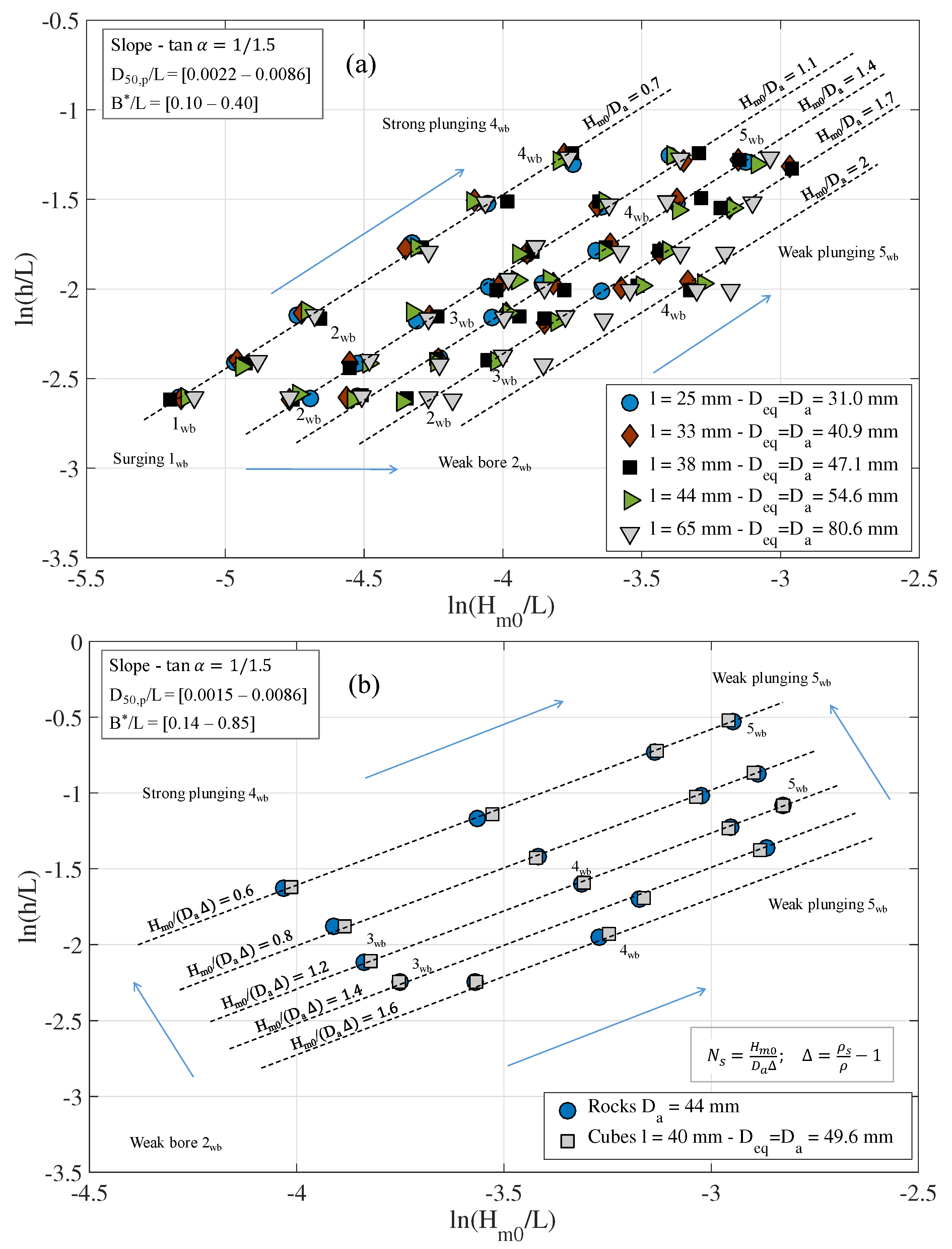
4.1. Observed Wave Breaker Type and the Non-Dimensional Parameter $H_{M0}/D_A$

Figure 4 show the experimental space of IISTA-UGR and Aalborg University but including the best fit lines of the the non-dimensional quantity $H_{m0}/D_a$ (dashed lines), and the most likely evolution of the wave breaker type following $H_{m0}/D_a$ isolines (blue lines), respectively.

Following Figure 4a, for $H_{m0}/D_a=0.7$, the wave breaker type likely evolves from surging to strong plunging, as both the relative water depth, $h/L$, and the steepness of the wave incident train, $H_{m0}/L$, increase. Following the isoline $H_{m0}/D_a=2$, the wave breaker type likely evolves from weak bore to weak plunging, as $h/L$ and $H_{m0}/L$ increase. Notice that during each experiment, the observed evolution of the wave breaker type depends on the fixed value of $h/L$, (constant wave period), while the wave height is increased, and, consequently, $H_{m0}/L$ and $H_{m0}/D_a$ increase too. Although there are much less experimental information, the same behavior is observed in AAU’s data (Figure 4b).

In summary, the way the experiments are carried out, that is, defining the sequence of wave height and wave period of each run, sets down the most likely type of observed wave breaking and its most probable evolution.

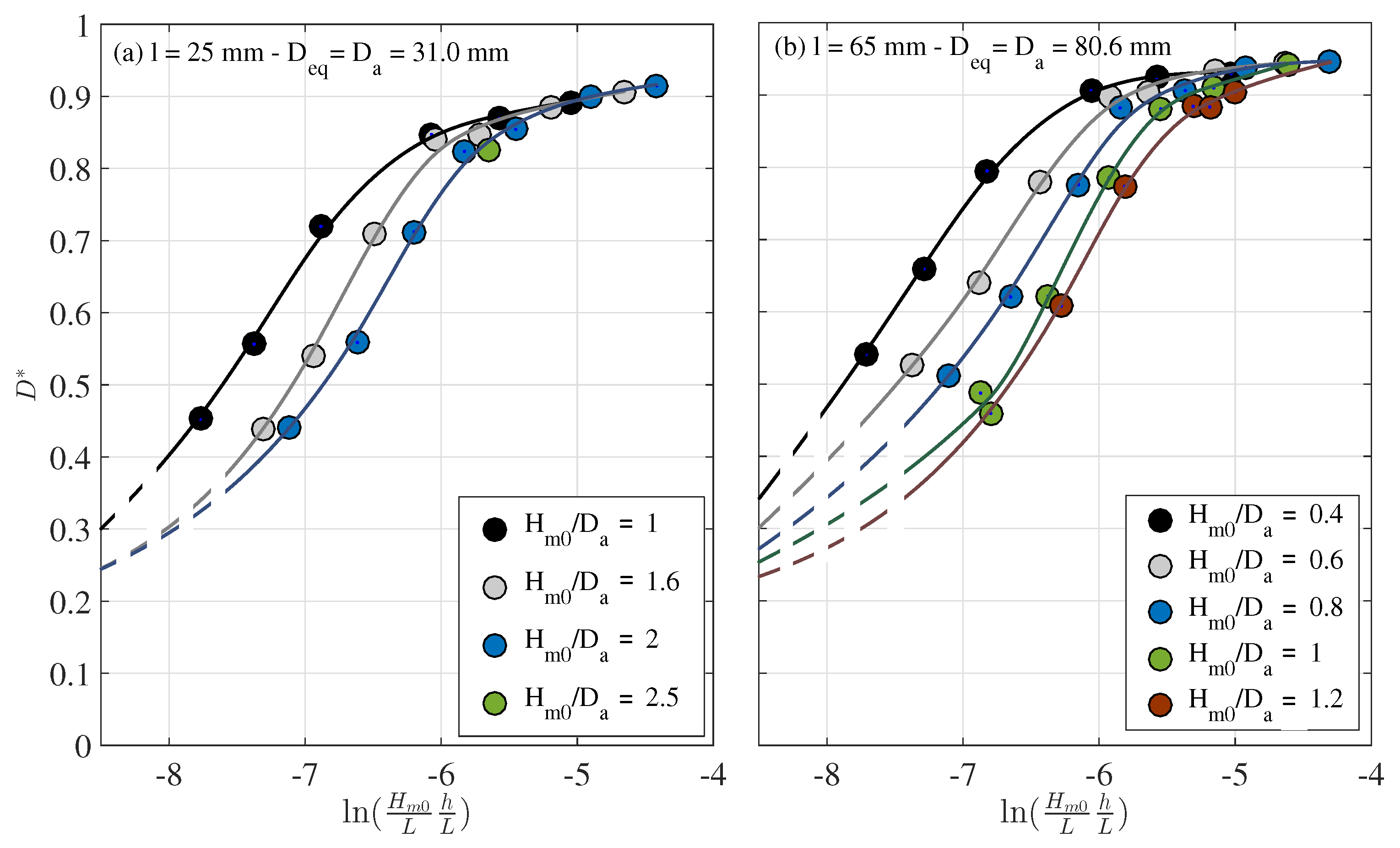
4.2. Dependence of the Bulk Dissipation on the Armor Unit

Based on the dimensional analysis (Equation (A4), Appendix A), Figure 5 shows the results of the bulk dissipation rate for two sizes of cubes tested in the wave flume of IISTA-UGR in function of the logarithmic transformation of the product $(h/L)(H_{m0}/L)$ (x-axis). As expected, the points are following curves of constant value of $H_{m0}/D_a$. The curves are fit using splines. The shape of the curve resembles the logistic sigmoid function [24] as correspond to a transport process in fluid mechanics [47], in this case, the transport of turbulence. The dashed lines represent the estimation of $D^{*}$ for very small values of ($h/L$)($H_{m0}/L$), that is, wave steepness, the dissipation should asymptotically tend to zero. Indeed, this non-dimensional quantity is a kind of Keulegan–Carpenter number [48].

The three regions of wave energy transformation are identified, namely: (i) dissipation-dominated region ($D^{*}>0.85$ and 0.95, respectively), (ii) reflected-dominated region ($D^{*}<0.30$ and 0.35, respectively), and (iii) transition region. Isolines converge in the dissipation-dominated region $ln\left[(h/L)(H_{m0}/L)\right]>-5.5$, regardless of $H_{m0}/D_a$ value, and the most likely breaker type is strong or weak plunging. The dissipative process is essentially dominated by the wave evolution and eventually wave-breaking on the free surface of the slope. For small values of $ln\left[(h/L)(H_{m0}/L)\right]<-7.5$ (reflected-dominated region), the curves converge to very low dissipation values, and the reflection in the slope and in the porous core is the main process of wave energy transformation. In this region, the most likely breaker type is a surging or weak bore. In the transition region, the bulk dissipation decreases significantly in a small range of $(h/L)(H_{m0}/L)$ values, depending on the value of $H_{m0}/D_a$, as well as the most likely type of wave-breaking.

This important conclusion is corroborated by AAU’s data. Figure 6 shows the results of the bulk dissipation of the two types of armor units tested, following the isolines of the non-dimensional number, $N_s=\frac{H_{m0}}{\mathsf{\Delta }{D}_a}$. In this case, the effect of the density is included because the comparison is between concrete cubes and natural rocks. The three regions of wave energy transformation can also be identified, but the absence of information weakens the potential interpretation. However, from a practical point of view, it is remarkable that the hydrodynamic performance of the two breakwaters with different armor units (rock of 44 mm and cubes of size 44 mm) are almost identical: (1) the range of $ln\left[(h/L)(H_{m0}/L)\right]$ of the three transformation regions is the same, (2) the variation of the bulk dissipation with $ln\left[(h/L)(H_{m0}/L)\right]$] is very similar, and consequently the reflected energy flux too, and (3) the most likely breaker types observed. In summary, from the hydrodynamic point of view both typologies can be exchanged. This result has too implications: it helps to optimize the breakwater (total cost analysis [2]) and makes doubt about the engineering application of the notional permeability parameter [30].

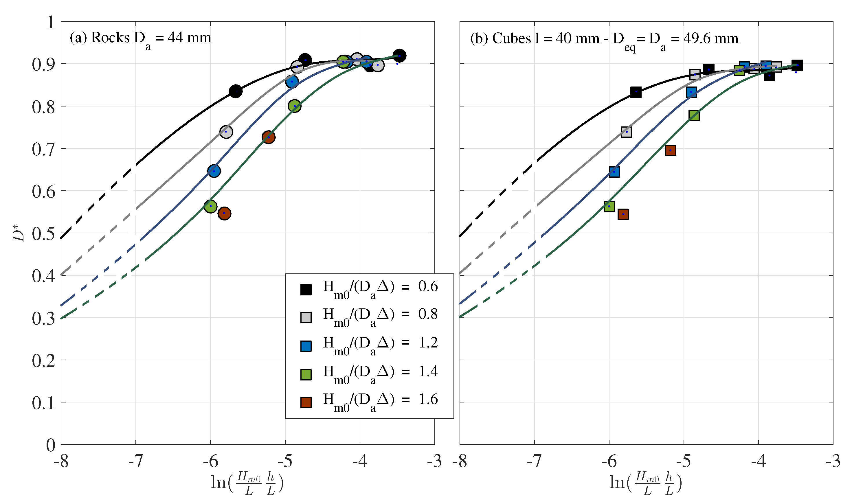
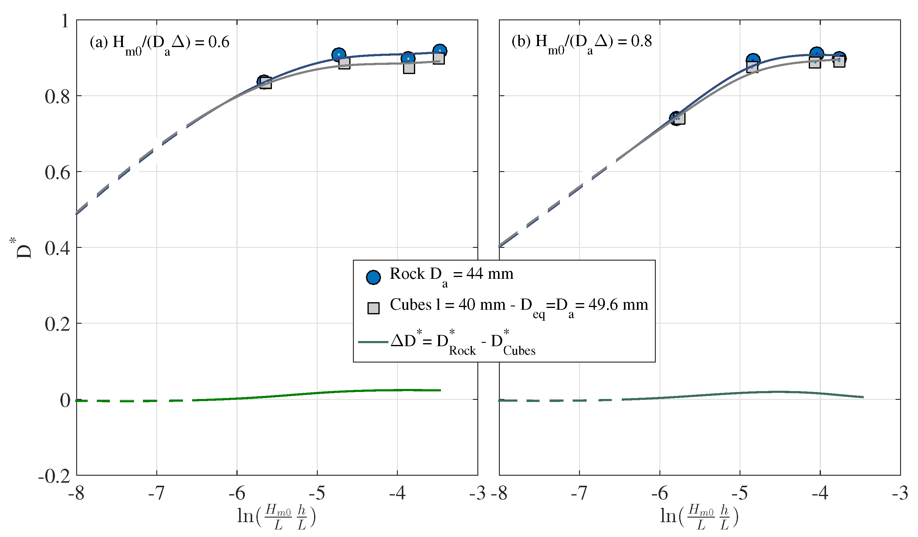
4.3. Comparative Bulk Dissipation between Different Sizes and Isolines $H_{M0}/D_A$ and $N_S$

Figure 7 and Figure 8 represents the bulk dissipation difference between breakwaters with different size or type of armor units for the main armor layer. According to Equation (6), this result can be associated with the different dissipation that the same wave train experiences in each main armor layer. For the experimental results of the double cubes armor layer (IISTA-UGR, five different sizes), the dissipation differences between the armor layer constructed with the larger unit size, $l=65$ mm, and the other four sizes of cubes is calculated (Figure 7). The bulk dissipation difference is noticeable only in the transition region reaching a maximum in an specific range of $(h/L)(H_{m0}/L)$ values. Moreover, the maximum value depends on $H_{m0}/D_a$, being larger as the value of the non-dimensional parameter decreases.

The comparison is between the larger cube size and the other ones for the same $H_{m0}/D_a$ value. Because the maximum difference occurs at a specific value of $(h/L)(H_{m0}/L)$, the ratio between wave heights is $H_{sm}=H_{65}(D_{sm}/D_{65})$ (being the sub-index $sm$ the smaller size), while h is constant, the wave length is different for each armor size,

$$L_{sm}/L_{65}=\sqrt{\frac{H_{sm}}{H_{65}}}=\sqrt{\frac{D_{sm}}{D_{65}}}$$

It is remarkable that the wave steepness is conserved (as well as the Iribarren number), however, the type of wave breaking is different for each cube size, and the bulk dissipation (per unit of incident wave energy) is larger in the breakwater built with the smaller size.

On the other hand, to get the same bulk dissipation, (say $D^{*}=0.90$), with slopes, one built with $D_{25}$ and the other one with $D_{65}$, the wave transformation processes are different. For the smaller cubes all the isolines of $H_{m0}/D_{25}$ collapse in a single curve, $ln\left[(h/L)(H_{m0}/L)\right]>-5$, and the most likely breaker type is weak plunging. For the larger cubes, all isolines, $0.4<H_{m0}/D_{25}<1.2$, cross the value $D^{*}=0.90$, and the most likely wave breaker types transit from strong to weak plunging, as $ln\left[(h/L)(H_{m0}/L)\right]>-6.2$.

Figure 8 shows, for AAU data, the difference between the two armor layer tested, double layer of rocks and cubes, calculated for $N_s=0.6$ (Figure 8a) and $N_s=0.8$ (Figure 8b). Because the armor units are of different material (rock and concrete respectively), the non-dimensional quantity includes the submerged relative density, $\mathsf{\Delta }=({\rho }_s/\rho )-1$, recovering the stability number, $N_s$. It can be seen that both set of data is collapsed in the same isoline of $N_s$. Based on the working hypothesis, it can be concluded that an armor layer built with rocks of $D_a=44$ mm and another one with concrete cubes of $D_a=D_{eq}=49.6$ mm, dissipate in the main layer almost the same amount of incident energy for the entire range of $(h/L)(H_{m0}/L)$.

5. Discussion

5.1. Assimilation of Data from Different Laboratories

The methodology presented in this paper can help in deciding whether two series of data obtained in different laboratories are assimilable or not. Three aspects are relevant: (1) the wave generation curve and the experimental space, ($h/L$, $H/L$), at the toe of the breakwater, (2) the location in the wave flume and the geometric scale of the models, and (3) the sequence of the experiment based on the generation variables T (or L) and H.

The generation curve of each wave flume can be extrapolated to the experimental space and check the pairs of values that match or not. The comparison should not be made with the target values sent to the paddle of generation, since the difference between the programmed and generated waves can be significant. On the contrary, it must be done with the values of the incident wave train obtained with the breakwater built and a method of separation of the incident, reflected and transmitted time series. Then, the energy conservation equation must be solved to determine the bulk dissipation. The second aspect determines the similarity of the wave transformation processes and the hydrodynamic performance of each breakwater. The scale helps to determine the hydrodynamic regimes in the slope, armor layer and core. Finally, the way that the experiment is carried out, that is, defining the sequence of wave height and wave period of each run, sets down the most likely type of observed wave breaking and its most probable evolution.

5.2. The Dependence on the Core: Characteristic Width and Grain Size

It is usual that water depth, characteristic width of the core ($B^{*}$) and size of the grain ($D_{50,p}$) are kept constant all along the experiment. Then, any of the three non-dimensional parameters $h/L$, $B^{*}/L$ or $D_{50,p}/L$ carry the same information about the hydrodynamic performance of the breakwater, if the slope does not change. Thus, the curve of the bulk dissipation $D^{*}$, Figure 5 and Figure 6, will be the same if plotted against $ln[(h/L)(H_{m0}/L)$, $ln[(B^{*}/L)(H_{m0}/L)$ or $ln[(D_{50,p}/L)(H_{m0}/L)$. Only the range of values of the x-axis would be different. However, for comparison of experiment results obtained in different laboratories, it is necessary to handle those values to check if the hydrodynamic regimes inside the porous medium are similar.

5.3. Bulk Dissipation and Armor Stability

Equation (A6) derived from the dimensional analysis in Appendix A provides the correlation between the bulk dissipation, $D^{*}$, and the stability number, $N_s$, which can be written as,

$$D^{*}=ln\left(\frac{h}{L}·\frac{H}{L}\right){\mathsf{\Psi }}_D\left[\left(N_s,R_{e,D_a}\right);\left(\frac{D_{50,p}}{L},\frac{B^{*}}{L},\frac{e}{L}\right)\right]$$

For a given breakwater, the slope angle, $D_{50,p}$ and $B^{*}$ are constant, and if the armor layer is built with the same thickness and the same placement procedure, then,

$$D^{*}=ln\left(\frac{h}{L}·\frac{H}{L}\right){\mathsf{\Psi }}_D\left(N_s,R_{e,D_a}\right)$$

Verifying that the armor stone Reynolds numbers are larger than a critical value, say $R_{e,D_a}>3·{10}^4$ [20,49], then

$$D^{*}=ln\left(\frac{h}{L}·\frac{H}{L}\right){\mathsf{\Psi }}_D\left(N_s\right)$$

or

$$N_s=ln\left(\frac{h}{L}·\frac{H}{L}\right){\mathsf{\Psi }}_{N_s}\left(D^{*}\right)=\varphi ·\mathsf{\Psi }$$

The bulk dissipation and the stability number are related, which does not affect the shape of the slope, plane or “damaged”, and the type of armor unit. $N_s$ mimics the performance of the bulk dissipation, and its values depends on the actual region, dissipation-dominated, reflection-dominated and transition. If the slope is damaged and, eventually, reaches a new stable shape, the reflected energy flux usually decreases and the bulk dissipation increases [34]. Notice that the correspondence between $D^{*}$ and $N_s$ is not biunivocal, and the function is not monotonic. On the contrary, it depends on (i) the relative water depth and wave steepness, (ii) the slope and its evolving shape (usually defined by the damage parameter, S), and (iii) the other quantities that define the geometry of the breakwater. Consequently, as the wave height grows, and if the wave period is constant, $(h/L)(H/L)$ and $H/D$ grows too.

5.4. Dissipation in the Main Layer and the Notional Permeability P

The dissipation in the armor layer depends basically on the size and shape of the armor units, the number of layers and the permeability underneath the armor layer. The results show the complexity of the processes of the turbulence transport and the wave energy dissipation in the permeable slope with main layer.

It is well-known that the armor layer stability depends on permeability. Van der Meer [30] incorporated the permeability in the stability formula of rock armor units through the so-called “notional permeability”, P. Four values of this coefficient (0.1, 0.4, 0.5 and 0.6) correspond to four different structures. Next, the parameter P was included in the stability formula and used as well as other coefficients to fit the final curve. Hence, the notional permeability is controversial, specifically because it does not solely depend on structural properties, but on the external forces as well. Therefore, the assumption that all the structures have a fixed P-value is fundamentally wrong [50]. In summary, the uncertainty of the P coefficient is dragged directly to the fitted formula.

Moreover, the present results not only confirm these conclusions, but show that the hydrodynamic performances of permeable structures, bulk dissipation and stability number, depend simultaneously on the wave steepness, the relative water depth, and the dynamic interaction with the structure, being the slope angle of an external parameter [37]. For the design of optimal breakwaters [2,33], it is highly recommended to develop a new stability formula based on the understanding of the complex processes of wave–structure interaction, quantifying the uncertainty and, consequently, being free of coefficients without physical meaning.

6. Conclusions

The main objective of this research was to analyze the dissipation process due to the interaction of the incident wave train with the main armor layer, and to quantify the performance between mound breakwaters built with different types and sizes of armor units. For that, the generalized $\mathsf{\Pi }$-Buckingham theorem is applied to properly construct the complete set of independent variables that specify the bulk dissipation and its components. Moreover, this work is supported by two series of data obtained experimentally in the wave flume of Aalborg University and also in the wave flume of IISTA, University of Granada. The latter are the experimental data presented in Clavero et al. [34]. The following conclusions can be derived from this study:

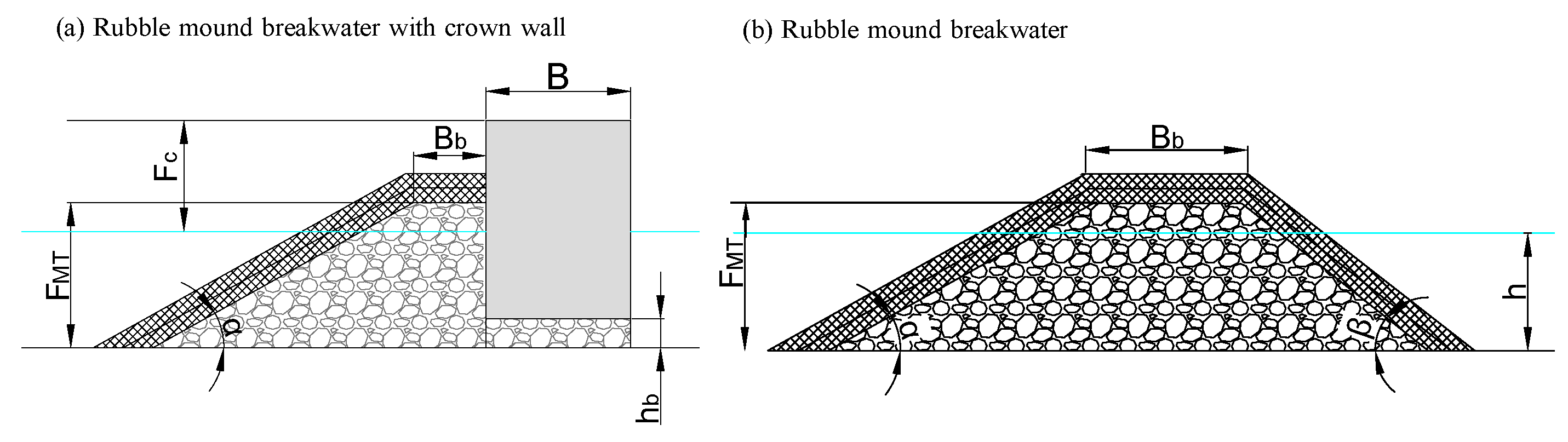
• The bulk dissipation depends on the turbulent regime generated in the main armor layer, which in turn depends on $(h/L)(H_{m0}/L)$, the relative size of the armor unit, $D_a/H$, the relative thickness, $e/L$, the shape and specific placement criterion, the characteristics of the porous core, $B^{*}/L$, $D_{50,p}/L$, and the slope angle of the breakwater.
• The dissipation of the incident energy in the main armor layer with different sizes of cubes is relevant at specific intervals of $(h/L)(H_{m0}/L)$, related to the transition region and the breaker type, from weak bore to strong plunging. The difference is negligible in the reflective and dissipative regions.
• The dissipation of the incident wave train in the armor layer composed of rocks and in the armor layer with cubes have, in practice, the same bulk dissipation over the entire range of $(h/L)(H_{m0}/L)$.
• For a given breakwater, that is, the slope angle, $D_{50,p}$ and $B^{*}$ are constant, and if the armor layer is built with the same thickness and placement criterion, the dimensional analysis provides a functional relationship between the number of stability of the armor unit and the bulk dissipation in the armor layer.
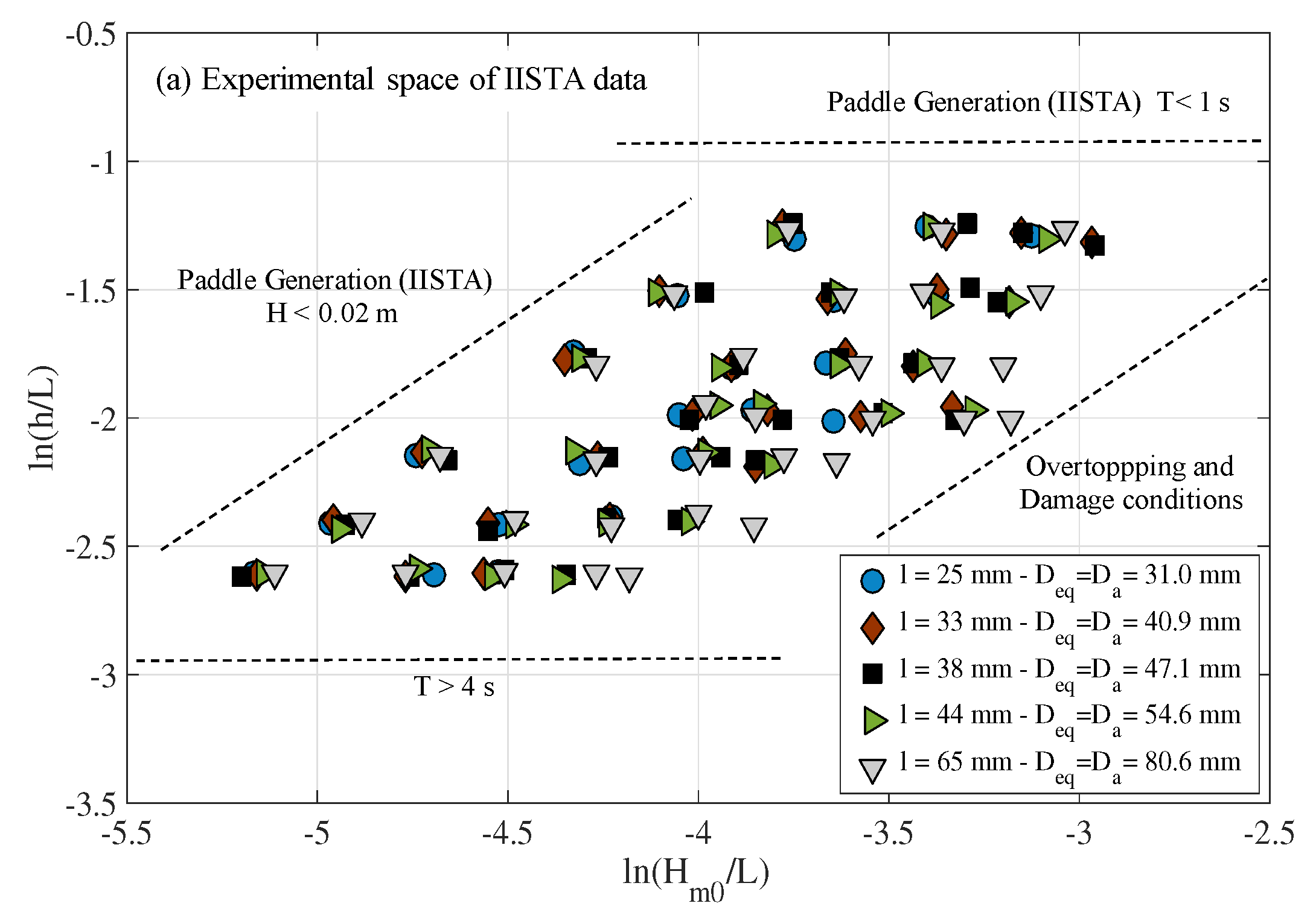
• For the experimental tests performed in the wave flume of IISTA, University of Granada, the experimental spaces are organized around lines parallel to the x-axis based on a constant $h/L$ value. The constant $H_{m0}/D_a$ lines determine an evolution of the breaker type in the sense of surging to weak plunging. Lower values of $H_{m0}/D_a$ offer a higher probability to observe all the breaker types.
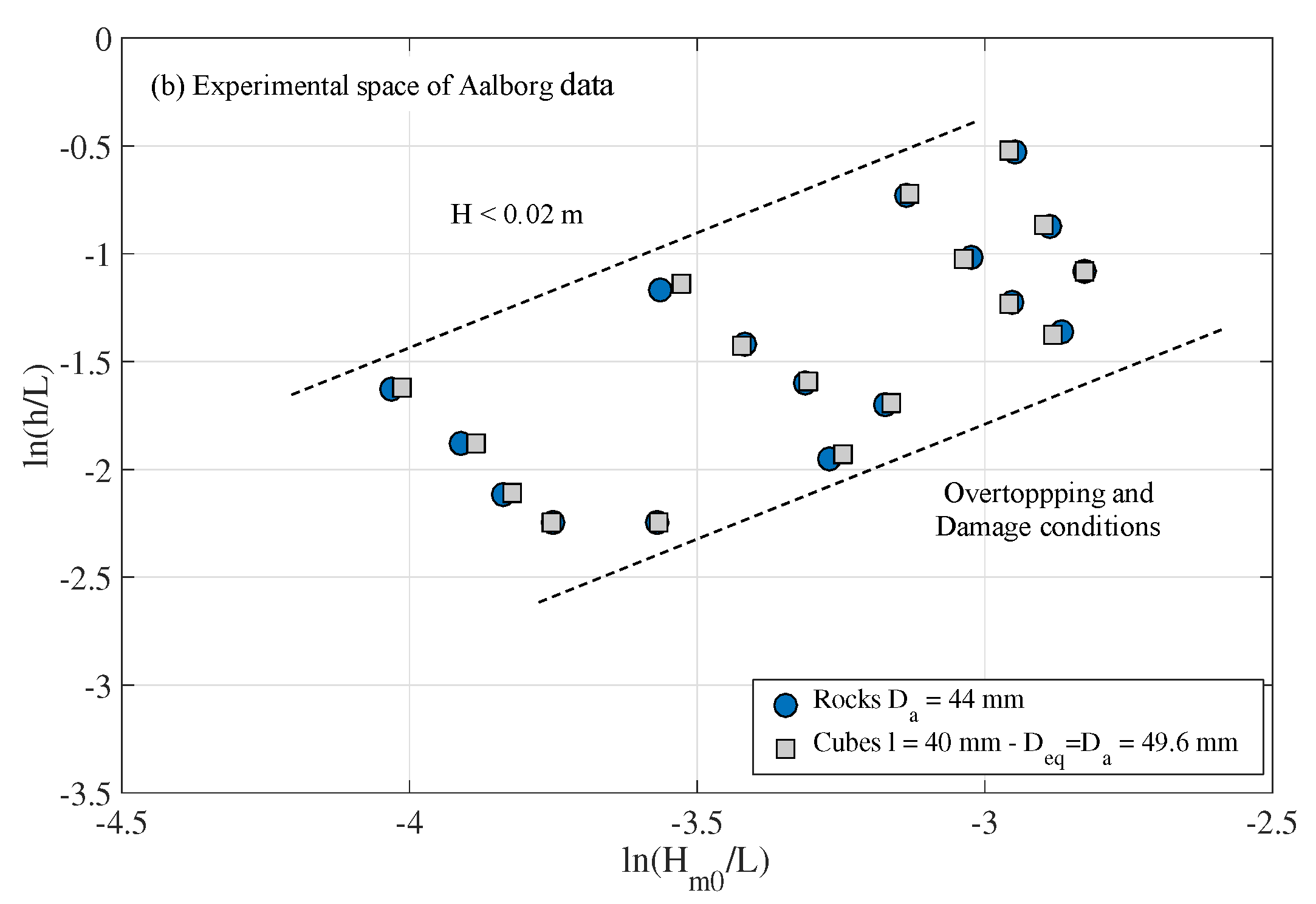
• The experimental technique of Aalborg University of keeping the Iribarren number constant is represented in the experimental space by trajectories parallel to the y-axis, that is, $ln(h/L)$. In addition, the physical limitations of the generation system and its control, make it difficult to comply with the constant Iribarren number requirement, so it cannot be assured that the experimentation collects all breaker types.

References

1. ROM 0.0-01. ROM 0.0. General Procedure and Requirements in the Design of Harbor and Maritime Structures; Puertos del Estado: Madrid, Spain, 2001; p. 218. [Google Scholar]
2. ROM 1.1-18. ROM 1.1. Recommendations for Breakwater Construction Projects; Puertos del Estado: Madrid, Spain, 2018. [Google Scholar]
3. Losada, M.; Díaz-Carrasco, P.; Moragues, M.; Clavero, M. Variabilidad intrínseca en el comportamiento de los diques rompeolas. In Proceedings of the 15th National Conference of Jornadas Españolas de Puertos y Costas, Torremolinos, Spain, 8–9 May 2019. [Google Scholar]
4. Christensen, E.; Deigaard, R. Large eddy simulation of breaking waves. Coast. Eng. 2001, 42, 53–86. [Google Scholar]
5. Lara, J.; Losada, I.; Liu, P. Breaking waves over a mild gravel slope: Experimental and numerical analysis. J. Geophys. Res. Atmos. 2006, 11, C11019. [Google Scholar]
6. Zhang, Q.; Liu, P. A numerical study of bore runup a slope. Adv. Eng. Mech. Reflect. Outlooks 2006, 265–285. [Google Scholar] [CrossRef]
7. Madsen, P.; Fuhrman, D. Run-up of tsunamis and long waves in terms of surf-similarity. Coast. Eng. 2008, 55, 209–223. [Google Scholar]
8. Gíslason, K.; Fredsoe, J.; Deigaard, R.; Sumer, B. Flow under standing waves: Part 1. Shear stress distribution, energy flux and steady streaming. Coast. Eng. 2009, 56, 341–362. [Google Scholar]
9. Lakehal, D.; Liovic, P. Turbulence structure and interaction with steep breaking waves. J. Fluid Mech. 2011, 674, 522–577. [Google Scholar]
10. Sollitt, C.; Cross, R. Wave transmission through permeable breakwaters. In Proceedings of the 13th International Conference on Coastal Engineering, Vancouver, BC, Canada, 10–14 July 1972; Volume 3, pp. 1827–1846. [Google Scholar]
11. Dalrymple, R.; Losada, M.; Martin, P. Reflection and transmission from porous structures under oblique wave attack. J. Fluid Mech. 1991, 224, 625–644. [Google Scholar]
12. Van Gent, M. Wave Interaction with Permeable Coastal Structures. Ph.D. Thesis, Delft University, Delft, The Netherlands, 1995. [Google Scholar]
13. Pérez-Romero, D.; Ortega-Sánchez, M.; Moñino, A.; Losada, M. Characteristic friction coefficent and scale effects in oscillatory flow. Coast. Eng. 2009, 56, 931–939. [Google Scholar]
14. Vílchez, M.; Clavero, M.; Lara, J.; Losada, M. A characteristic friction diagram for the numerical quantification of the hydraulic performance of different breakwater types. Coast. Eng. 2016, 114, 86–98. [Google Scholar]
15. Kobayashi, N.; Wurjanto, A. Irregular Wave Interaction with Permeable Slopes. In Proceedings of the 23rd International Conference of Coastal Engineering, ASCE, 118, Venice, Italy, 4–9 October 1992; pp. 368–386. [Google Scholar]
16. Lara, J.; Losada, I.; Guanche, R. Wave interaction with low-mound breakwaters using a RANS model. Ocean Eng. 2008, 35, 1388–1400. [Google Scholar]
17. Van Gent, M. Rock stability of rubble mound breakwaters with a berm. Coast. Eng. 2013, 78, 35–45. [Google Scholar]
18. Ruju, A.; Lara, J.; Losada, I. Numerical analysis of run-up oscillations under dissipative conditions. Coast. Eng. 2014, 86, 45–56. [Google Scholar]
19. Jensen, B.; Christensen, E.; Sumer, B. Pressure-induced forces and shear stresses on rubble mound breakwater armour layers in regular waves. Coast. Eng. 2014, 91, 60–75. [Google Scholar]
20. Jensen, B.; Jacobsen, N.; Christensen, E. Investigations on the porous media equations and resistance coefficients for coastal structures. Coast. Eng. 2014, 84, 56–72. [Google Scholar]
21. Vanneste, D.; Troch, P. 2D numerical simulation of large-scale physical model tests of wave interaction with a rubble-mound breakwater. Coast. Eng. 2015, 103, 22–41. [Google Scholar]
22. Scarcella, D.; Benedicto, M.; Moñino, A.; Losada, M. Scale effects in rubble mound breakwaters considering wave energy balance. In Proceedings of the 30th Coastal Engineering Conference, San Diego, CA, USA, 3–8 September 2006; pp. 4410–4416. [Google Scholar]
23. Zanuttigh, B.; Van der Meer, J. Wave reflection from coastal structures in design conditions. Coast. Eng. 2008, 55, 771–779. [Google Scholar]
24. Vílchez, M.; Clavero, M.; Losada, M. Hydraulic performance of different non-overtopped breakwater types under 2D wave attack. Coast. Eng. 2016, 107, 34–52. [Google Scholar]
25. Moragues, M.; Clavero, M.; Losada, M. Flow characteristics on impermeable and permeable slopes: A synthesis for design. Coast. Eng. 2019. submitted. [Google Scholar]
26. Iribarren, C.; Nogales, C. Protection des Ports. Presented at the 17th International Navigation Congress, Permanent Int., S. II-C.4, Lisbon, Portugal, 1 January 1949. [Google Scholar]
27. Iversen, H. Gravity Waves. Laboratory study of breakers. In Circular of the Bureau of Standards; National Bureau of Standards: Gaithersburg, MD, USA, 1952; Volume 521, pp. 9–32. [Google Scholar]
28. Cyril, J.; Galvin, J. Break type classification on the three laboratory beaches. J. Geophys. Res. 1968, 73, 13651–13659. [Google Scholar]
29. Battjes, J. Surf Similarity. In Proceedings of the 14th International Conference on Coastal Engineering, Copenhagen, Denmark, 24–28 June 1974; pp. 466–480. [Google Scholar]
30. Van der Meer, J.W. Rock Slope and gravel Beaches Under Wave Attack. Ph.D. Thesis, Delft University, Delft, The Netherlands, 1988. [Google Scholar]
31. Van der Meer, J.; Van Gent, M.; Wolters, G.; Heineke, D. New Design Guidance for Underlayers and Filter Layers for Rock Armour under Wave Attack; ICE Publishing: London, UK, 2018. [Google Scholar]
32. Eldrup, M.; Andersen, T.; Burcharth, H. Stability of rubble mound breakwaters-A study of the notional permeability factor, based on physical model tests. Water (Switzerland) 2019, 11, 934. [Google Scholar]
33. PIANC-196. Criteria for the Selection of Breakwater Types and Their Related Optimum Safety Lavels; The Worls Association for Waterborne Transport Infraestructure: Brussels, Belgium, 2016. [Google Scholar]
34. Clavero, M.; Folgueras, P.; Díaz-Carrasco, P.; Ortega-Sánchez, M.; Losada, M. A similarity parameter for breakwaters: The modified Iribarren number. In Proceedings of the 36th International Conference on Coastal Engineering, Baltimore, MD, USA, 30 July–3 August 2018. [Google Scholar]
35. Bruun, P.; Günbak, A. Stability of sloping structures in relation to ξ = tanα/ H / L o risk criteria in design. Coast. Eng. 1977, 1, 287–322. [Google Scholar]
36. Losada, M.; Giménez-Curto, L.A. The joint effect of the wave height and period on the stability number of rubble mound breakwaters using Iribarren’s number. Coast. Eng. 1979, 3, 77–96. [Google Scholar]
37. Díaz-Carrasco, P.; Moragues, M.; Clavero, M.; Losada, M. 2D Water-wave interaction with permeable and impermeable slopes: Dimensional analysis and experimental overview. Coast. Eng. 2020. accepted. [Google Scholar]
38. Ting, F.; Kirby, J. Dynamics of surf-zone turbulence in a spilling breaker. Coast. Eng. 1996, 27, 131–160. [Google Scholar]
39. Sonin, A. The Physical Basis of Dimensional Analysis, 2nd ed.; Department of Mechanical Engineering, MIT, Cambridge: Cambridge, MA, USA, 2001. [Google Scholar]
40. Díaz-Carrasco, P.; Eldrup, M.; Andersen, T. Wave-Breakwater Interaction: Test Program in the Flume of Aalborg University; Technical documentation; Department of Civil Engineering, Aalborg University: Aalborg, Denmark, 2019. [Google Scholar]
41. CIRIA; CUR; CETMEF. The Rock Manual: The Use of Rock in Hydraulic Engineering; CIRIA: London, UK, 2007; p. C683. [Google Scholar]
42. Aalborg University. AwaSys—Software for Wave Laboratories; Aalborg University: Aalborg, Denmark, 2018. [Google Scholar]
43. Baquerizo, A. Reflexión del Oleaje en Playas. Métodos de Evaluación y de Predicción. Ph.D. Thesis, University of Cantabria, Cantabria, Spain, 1995. [Google Scholar]
44. Eldrup, M.; Andersen, T. Estimation of incident and reflected wave trains in highly nonlinear tho dimensional irregular waves. J. Waterw. Port Coast. Ocean Eng. 2019, 145, 04018038. [Google Scholar]
45. Frigaard, P.; Brirsen, M. A time-domain method for separating incident and reflected waves. Coast. Eng. 1995, 24, 205–215. [Google Scholar]
46. Frigaard, P.; Andersen, T.L. Analysis of Waves: Technical Documentation for WaveLab 3; DCE Lecture notes, No. 33; Aalborg University: Aalborg, Denmark, October 2014; Available online: https://vbn.aau.dk/en/publications/ (accessed on 26 February 2020).
47. Churchill, S.; Usagi, R. A general expression for the correlation of rates of transfer and other phenomena. AICHE J. 1972, 18, 1121–1128. [Google Scholar]
48. Dixen, M.; Hatipoglu, F.; Sumer, B.; Fredsoe, J. Wave boundary layer over a stone-covered bed. Coast. Eng. 2008, 55, 1–20. [Google Scholar]
49. Dai, Y.; Kamer, A. Scale Effect Tests for Rubble Mound Breakwaters; Research Report H-69-2; U.S. Army Engineer Waterway Experiment Station, Corps of Engineers: Vicksburg, MI, USA, 1969. [Google Scholar]
50. Van der Neut, E. Analysis of the Notional Permeability of Rubble Mound Breakwaters by Means of a VOF Model. Ph.D. Thesis, Delft University, Delft, The Netherlands, 2015. [Google Scholar]
51. Kortenhaus, A.; Oumeraci, H. Classification of wave loading on monolithic coastal structures. Coast. Eng. 1998, 26, 867–880. [Google Scholar]
Figure 1. Scheme of the wave flumes of: (a) IISTA—University of Granada—23 × 0.65 × 1 m (dimensions in meters), and (b) Aalborg University—21.5 × 1.2 × 1.5 m (dimensions in centimeters). The location of wave gauges positioned in each laboratory is included.
Jmse 08 00152 g001
Figure 2. Physical model of the breakwater tested: (a) IISTA-UGR, rubble-mound breakwater with crown wall; (b) Aalborg University, a conventional rubble-mound breakwater.
Jmse 08 00152 g002
Figure 3. The log-experimental space [ ln ( h / L ) , ln ( H m 0 / L ) ] of (a) IISTA—University of Granada, and (b) Aalborg University. Dashed lines represent the experimental limits for wave generation, and non-overtopping and non-damage conditions in the laboratories.
Jmse 08 00152 g003aJmse 08 00152 g003b
Figure 4. The log-experimental space [ ln ( h / L ) , ln ( H m 0 / L ) ] of the experimental results obtained from (a) IISTA, University of Granada, and (b) Aalborg University. The dash line represents the best fit of H m 0 / D a and H m 0 / ( Δ D a ) for the data of IISTA-UGR and Aalborg University, respectively. The trajectory and the most likely breaker type of some tests are also identified by numbers with the subindex w b : 1 = surging, 2 = weak bore; 3 = strong bore; 4 = strong plunging; 5 = weak plunging; 6 = spilling. See Appendix A for details.
Jmse 08 00152 g004
Figure 5. Bulk dissipation results against the log-transformation [( h / L )( H m 0 / L )] for two sizes of cubes, IISTA-UGR data: (a) Size of l = 25 mm and equivalent diameter D e q = D a = 31.0 mm, (b) Size of l = 65 mm and equivalent diameter D e q = D a = 80.6 mm. The solid lines represent the fit spline curve and the dashed lines marks the estimated asymptotic trend of bulk dissipation for very small values of ln [ ( h / L ) ( H m 0 / L ) ].
Jmse 08 00152 g005
Figure 6. Bulk dissipation results against the log-transformation [( h / L )( H m 0 / L )] for two types of unit pieces, Aalborg University data: (a) Rocks D a = 44 mm, (b) Cubes D e q = D a = 40 mm. The solid lines represent the fit spline curve and the dashed lines marks the estimated asymptotic trend of bulk dissipation for very small values of ln [ ( h / L ) ( H m 0 / L ) ] .
Jmse 08 00152 g006
Figure 7. The bulk dissipation results against the log-transformation of the product ( h / L )( H m 0 / L ) for all the cubes tested in the wave flume of IISTA-UGR according to (a) isolines of H m 0 / D a = 1.00 , (b) isolines of H m 0 / D a = 1.20 . The solid lines represent the fit spline curve and the dashed lines marks the estimated values of bulk dissipation for a small values of ln [ ( h / L ) ( H m 0 / L ) ]. The solid lines with values of D * < 0.3 represent the dissipation difference between the armor constructed with the larger size, l = 65 mm, and the other four sizes of cubes.
Jmse 08 00152 g007
Figure 8. The bulk dissipation results against the log-transformation of the product ( h / L )( H m 0 / L ) for cubes and rocks tested in the wave flume of Aalborg University according to (a) isolines of N s = H m 0 / ( Δ D a ) = 0.6 , (b) isolines of N s = H m 0 / ( Δ D a ) = 0.8 . The solid lines represent the fit spline curve and the dashed lines marks the estimated values of bulk dissipation for a small values of ln [ ( h / L ) ( H m 0 / L ) ]. The green solid line represents the dissipation difference between the rocks and the cubes.
Jmse 08 00152 g008