1. Introduction
A crucial task for an Autonomous Underwater Vehicle (AUV) is to build a map of the environment and to estimate its own pose within the map while it is navigating. This task is known as Simultaneous Localization and Mapping (SLAM) [
1] and is nowadays a de facto standard for autonomous vehicles, not only in underwater environments.
Since well-established approaches to SLAM, such as Extended Kalman Filter SLAM (EKF-SLAM) or Graph-SLAM [
2], are widely used and new approaches mainly concentrate on alleviating their intrinsic limitations [
3], SLAM is often considered a solved problem. New research tends to focus on practical- and application-related issues, which depend on or are strongly related to the sensors used to build the map and to estimate the vehicle motion and pose.
Range sensors, such as laser range finders in terrestrial environments or sonar in underwater scenarios, were the modality of choice at first. However, research turned to computer vision as soon as the computational capabilities and price of on-board systems made it possible [
4], since cameras provide a much richer representation of the world.
Underwater computer vision poses several problems [
5] that only exist up to a much lesser extent in other environments. That is why underwater SLAM solely based on vision [
6] is not frequent, as it requires approaches far more robust than its terrestrial counterparts. Visual SLAM and the associated visual loop closing detection processes are usually included in the navigation systems of AUV equipped with other sensors to mitigate the localization drift obtained when navigating only with inertial units (gyroscopes, magnetometers, and accelerometers), visual odometers, or Doppler Velocity Log (DVL) sensors.
However, large-scale or long time operations generate big maps with huge amounts of visual data that can collapse the vehicle computer if they are not treated intelligently [
7,
8]. A common strategy to overcome this problem is to explore the areas of interest in different, separated, missions called sessions [
9,
10,
11]. Any low capability of a robot to operate robustly during long periods of time can be alleviated by repeating transits through previously visited areas and by joining all trajectories in a single coordinate frame. When SLAM is performed in these conditions, it is referred to as multi-session SLAM.
In the context of the Augmented Reality Subsea Exploration Assistant (ARSEA) and Twin Robots (TWINBOT) national projects, one or several robots equipped with cameras have to operate cooperatively in tasks such as (a) sea bottom exploration, mapping, and mosaicking for biologic purposes and (b) multi-robot coordinated intervention. All these tasks are done in marine areas which are densely colonized with seagrass and, in particular, with Posidonia oceanica (see further details in
Section 10.1). In both projects, multi-session SLAM will be indispensable to aggregate the mapping data computed by all robots that participate in the missions.
Besides, several challenges come up when working in medium and large underwater areas colonized with seagrass, complicating the calculus of visual odometry and loop closings, namely (a) intricate textures; (b) slight dynamics due to the slow oscillation of the seagrass leaves with the water currents; (c) nonexistence of structured scenarios; and (d) lighting and visual hindrances, such as water turbidity, light scattering, flickering, and lack of natural light and visibility in deeper zones.
Furthermore, it is necessary to consider that (1) multi-session SLAM loops between different sessions, known as global loops, are continuously searched during the AUV operation. Therefore, reducing the computational cost of global image matching is crucial. (2) The advantages and drawbacks of the existing approaches for map joining define a compromise between map consistency and computation time; for example, building a full map mixing different sessions leads to more consistency than anchor-node-based solutions [
9] at the cost of significantly larger computation times.
This paper presents a novel trajectory-based multi-session visual SLAM and map joining approach which pays special attention on a frontend that searches intersession and intra-session loop closings and a backend to run the single and the global map optimizations. The relevant points and contributions are summarized next:
The application of a multi-session loop detector that uses the Hash-Based Loop Closure (HALOC) [
12] image global signature (hash) for fast-matching solves the problem of lacking geometry information between different sessions at a considerable speed; as a matter of fact, Negre Carrasco et al. [
12] has already shown that HALOC improves the loop closing detection performance with respect to Fast Appearance-Based Mapping (FABMAP) [
13] in terms of perceptual aliasing, execution time, and recall and especially in underwater environments.
The use of a hash to represent images for multi-session loop closing implies a considerable reduction of data to store and exchange between two different robots, when this application is extended (in forthcoming work) to a multi-robot context. This data reduction will be crucial to make feasible multi-session or multi-robot operations where one robot assumes the task to join all the maps of all robots that participate in the mission.
A novel and simple algorithm to join multiple map sessions: This system does not use anchor nodes but it joins two maps through a transformation between the end of one trajectory and the beginning of the other, solving, at the same time, and automatically the-so called initial state problem.
A strategy to perform delayed global map optimization (for map joining) to reduce computational load
A complete set of software sources available for the scientific community in GitHub public repositories [
14,
15,
16]
A wide set of experiments conducted in Mediterranean marine scenarios, mostly colonized with Posidonia oceanica, which show the validity and robustness of the localization system
To the best of our knowledge, such a trajectory-based approach to multi-session SLAM focused on marine bottoms colonized with seagrass has not been proposed before in the robotic literature.
The paper is structured as follows.
Section 2 summarizes the existing research on the subject.
Section 3 overviews our proposal, its main components, and how they relate to each other.
Section 4 summarizes the notation used throughout the paper.
Section 5 describes the block in charge of performing visual odometry. While performing visual odometry, both intra-session and intersession loops are detected as described in
Section 6 and
Section 7, respectively. These loops make it possible to optimize the trajectories as described in
Section 8 and to join them as stated in
Section 9. Finally,
Section 10 presents an extensive set of experimental results using real data gathered in several areas of Mallorca (Spain). The conclusions and some insight for further work are provided in
Section 11.
2. Related Work
The so-called initial state problem or kidnapped robot problem [
17] refers to the fact that, when a robot starts a new session on the same or in a partially overlapping nearby environment, it does not know its relative pose with respect to another map created previously. One possibility to solve this issue is to localize itself in any map built beforehand. This solution has the advantage of maintaining a single track and a single reference frame. However, this alternative has a strong restriction: the robot must start in a point already mapped. The other possibility is to initiate another map corresponding to this new session, with its own local reference, and then, when the robot detects a point already visited during a previous session, it calculates the transformation between both maps and joins them. This last strategy is known formally as the problem of multi-session simultaneous localization and mapping (SLAM) [
18] and consists in combining multiple SLAM trajectories obtained repeatedly over time in the same area by a single or several robots.
In this context, the challenges are basically two: (1) join properly maps gathered in different sessions based on their overlapping parts and (2) improve the current pose and map estimates using previous sessions’ data. In general, the aforementioned two main goals are achieved thanks to three building blocks: a visual odometer [
19] that matches consecutive images and provides local motion estimates, a loop detector [
12,
20] that asserts if the autonomous underwater vehicle (AUV) returns to a previously visited place, and an optimizer [
21,
22] that fuses odometry and loops to consistently improve and join maps as well as to properly estimate the AUV pose. Additional problems appear in multi-session localization because images gathered in several sessions can be extremely different due to changes in the illumination conditions [
5] or even the use of different cameras or AUVs.
Existing vision-based multi-session SLAM approaches are mainly focused on terrestrial and aerial environments. Some of them are based on the anchor-nodes method [
23], which introduces two main concepts: (a) robot trajectory
anchor, as the offset of a complete trajectory with respect to a global system of coordinates, and (b) an
encounter, defined as a measurement or transformation that connects two different poses of two different robots; in multi-session SLAM, the encounters are not direct transforms between robots but indirect via observations of the same area performed at different times. Encounters express additional constraints relating different graphs corresponding to different sessions. For example, McDonald et al. [
9] presents a multi-session stereo-vision SLAM approach based on anchor-nodes for indoor and outdoor terrestrial environments.
Contrarily to single session SLAM, multi-session loop detection (i.e., finding encounters) cannot rely on the AUV pose to constrain the search since, at first, the relative pose between sessions is unknown. Instead, global image descriptors [
24] such as
Bag of Words (BoW) are often used. In McDonald et al. [
9], the loop closings are detected using a BoW-based solution combined with Incremental Smoothing and Mapping (iSAM) [
25] for batch map optimization and Conditional Random Fields (CRF) [
26] for feature matching. In [
10,
27], a new memory management is presented in order to optimize the treatment of the successive graph nodes in multi-session mapping and path planning applications for large-scale indoor office-like environments, using a robot equipped with a RGBD camera and a laser scanner. BoW is used to detect visual global loop closings, the Tree-Based Network Optimizer (TORO) [
28] for graph optimization and the laser together with the RGBD point clouds for map visualization. Latif et al. propose in Reference [
29] a new algorithm for loop closure verification in single and multi-session pose graph connectivity: odometry is obtained by means of laser scan matching, with the loop closing candidates using BoW and the
g2o [
21] framework for graph optimization.
All the aforementioned references have been tested only in terrestrial environments, some indoors and outdoors and others only indoors. The literature is extremely scarce in multi-session SLAM addressed, implemented, and tested in underwater scenarios with AUVs. References [
18,
30,
31] are some of the very few pieces of work with these characteristics. The work presented in References [
30,
31] was designed for the very specific purpose of ship hull inspection and surveillance using AUVs. In this case, the robot moves around the ship hull, at a fixed distance to it, with the camera and the Doppler velocity log (DVL) pointing nadir to the hull. Planes fitting sparse 3-D point clouds obtained by the DVL are used to map the surface, and, in cooperation with a camera, to do single and multi-session SLAM. The Fast Appearance-Based Mapping (FABMAP) [
13] framework, which is based on BoW, is used for visual loop closing detection and anchor nodes for the map joining task. However, that field application is far from the scope of the work presented in our study.
The work presented by Williams et al. in Reference [
18] is closer to ours in the sense that the surroundings of an ancient shipwreck are surveyed by an AUV that records video sequences for visual mapping and 3-D reconstruction. The vehicle moves over the bottom, with a camera pointing downwards. The different portions of the shipwreck grabbed in different sessions are joined together in a single map using multi-session SLAM techniques.
3. Overview
This section summarizes our proposal. On the one hand, it introduces the main building blocks and the relationships among them. On the other hand, it provides some details to ease further reading and emphasizes the advantages and fields of application of the presented approach.
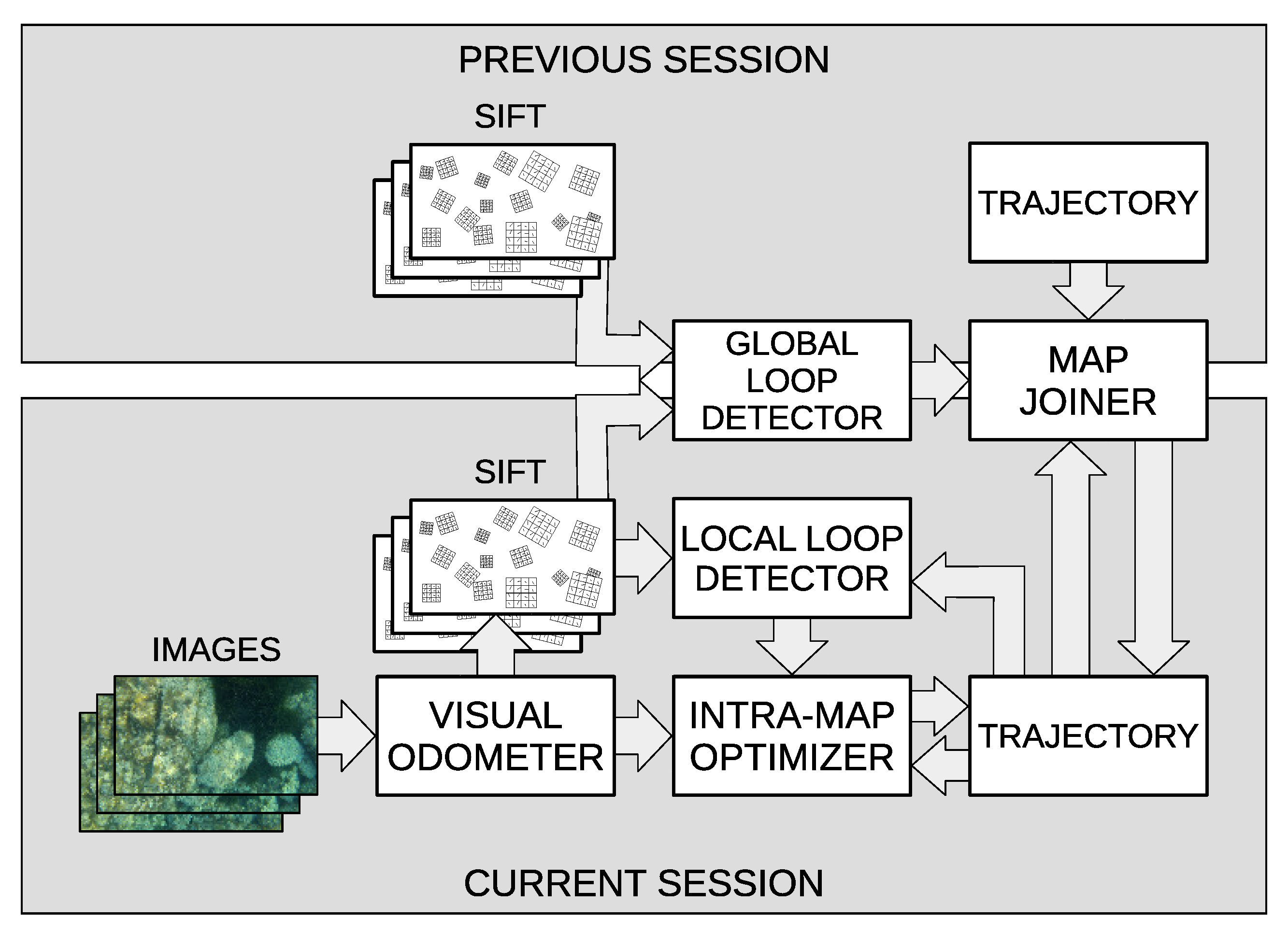
Our proposal, summarized in
Figure 1, focuses on the three building blocks of multi-session visual SLAM, paying special attention to robust and fast place recognition and facilitating the trade-off between consistency and speed. Moreover, our proposal is solely based on vision sensors and an altitude sensor for the pixel/meters scale computation. There is no need for dead reckoning devices.
A simple yet robust visual odometer based on Scale-Invariant Feature Transform (SIFT) [
32] is first described. Its output is used to build the so-called trajectory, which is a set of relative motion estimates between consecutive images.
Two loop detectors are introduced afterwards: the local loop detector, which is in charge of detecting loop candidates inside a region of interest around the AUV in one single session, and the global loop detector, which uses image hashes to find loop candidates between different sessions without any geometrical constraint. In both cases, candidates are confirmed by means of feature matching and Random Sample Consensus (RANSAC) [
33].
When used as global image descriptors, image hashes are functions providing fixed length outputs that are similar only in front of similar images [
34]. The multi-session loop closing detection task compares image hashes of images of different sessions. Hashes are obtained with HALOC [
12] because this approach reduces the perceptual aliasing inherent to clustering algorithms such as BoW [
12], it outperforms previous approaches in terms of reliability and computation time, it is particularly well suited in challenging underwater scenarios [
35], and it allows a very fast image comparison. Moreover, since the SIFT features used by HALOC have already been computed to perform visual odometry, requiring them does not compromise the execution time.
Two methods based on Extended Kalman Filters (EKF) are used to optimize the trajectories. The first one is the
intra-map optimizer and is in charge of improving the existing trajectory by means of the local loops. The second one is the
map joiner, of which the goal is to join different sessions while keeping the intrinsic trajectory structure. The computational complexity [
1] of the intra-map optimizer EKF is strongly reduced with respect to other approaches, since the trajectory based approach [
6] makes the state vector grow at a significantly lower rate. As for the map joiner EKF, it has a constant execution time because its state has a fixed size. In both cases, linearization errors are alleviated by iteratively re-linearising over subsequent EKF estimates, that is, using an Iterated EKF (IEKF).
The adopted optimization strategies have the following advantages: (a) They allow delayed loop closings, making it possible to store loop data and to optimize the trajectory or join different sessions only when enough computational resources are available; (b) as sessions are joined using a single link, the overhead introduced to join the maps is almost negligible. Moreover, this single linkage approach makes it possible to disaggregate the sessions easily to reduce the computation time when necessary, and (c) contrarily to pose-based SLAM approaches [
36], which play with global poses, this approach composes the trajectory with relative motions; then, EKF linearization problems are less relevant since motion covariances are disaggregated and only those involved in each loop take part in the process.
In order to increase the reproducibility of the presented results and to facilitate the use of our algorithms, the whole source code related to the research in this paper has been made publicly available. The links to each specific piece of code are provided throughout the paper.
4. General Notation
Even though specific notation will be introduced when needed, there are some common conventions that are pervasively used throughout the paper. This section focuses on such general notation and can be used as a reference to better understand further sections.
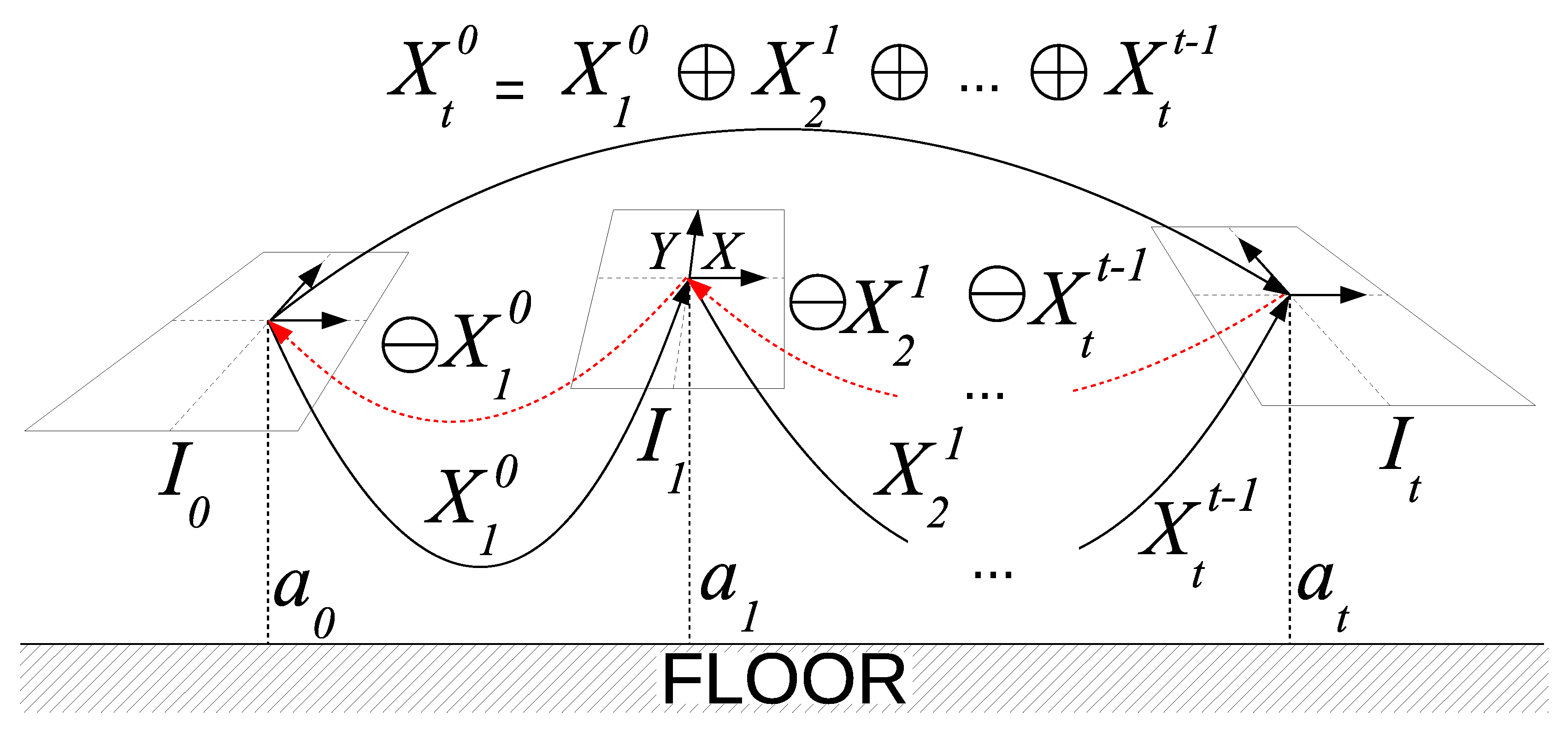
Let denote the image grabbed by the camera at time step t, with its coordinate frame placed at its center with the X and Y axes pointing forward and left, respectively. Also, let denote the altitude at which the image was grabbed. This study assumes that is obtained by external means, such as a stereo-vision altimeter or a DVL. Let us assume also that the underwater vehicle is programmed to navigate at a constant altitude, in an approximated horizontal plane, simplifying the robot motion to a 2-D trajectory.
The normal distribution models the roto-translation from image to image , with as its mean and as its covariance. Assuming a bottom-looking camera with negligible pitch and roll, can be expressed as a motion in X () and Y () and a rotation over Z (). That is, .
The trajectory is defined as the set of motions between consecutively grabbed images that fully define the path followed by the AUV. Our proposal is to model the trajectory at time t as , so that , shown in Equation (1), denotes the mean of and so that is the associated covariance matrix.
Equation (2) shows how the relative motion
between two arbitrary time steps
i and
j can be recovered as a normal distribution by means of the compounding ⊕ and inversion ⊖ operators as described in Smith et al. [
37].
The absolute pose
, which is the pose at time step
t relative to the first image, can be easily recovered from the trajectory using the previous equation.
Figure 2 summarizes the notation.
5. Visual Odometry
This section centers its attention on the visual odometer, which is in charge of providing local motion estimates between pairs of consecutively gathered images. Our proposal makes use of SIFT feature matching and RANSAC to provide local motions as accurate as possible.
Visual odometry consists of computing the motion
between images
and
taken by the robot camera at time instants
and
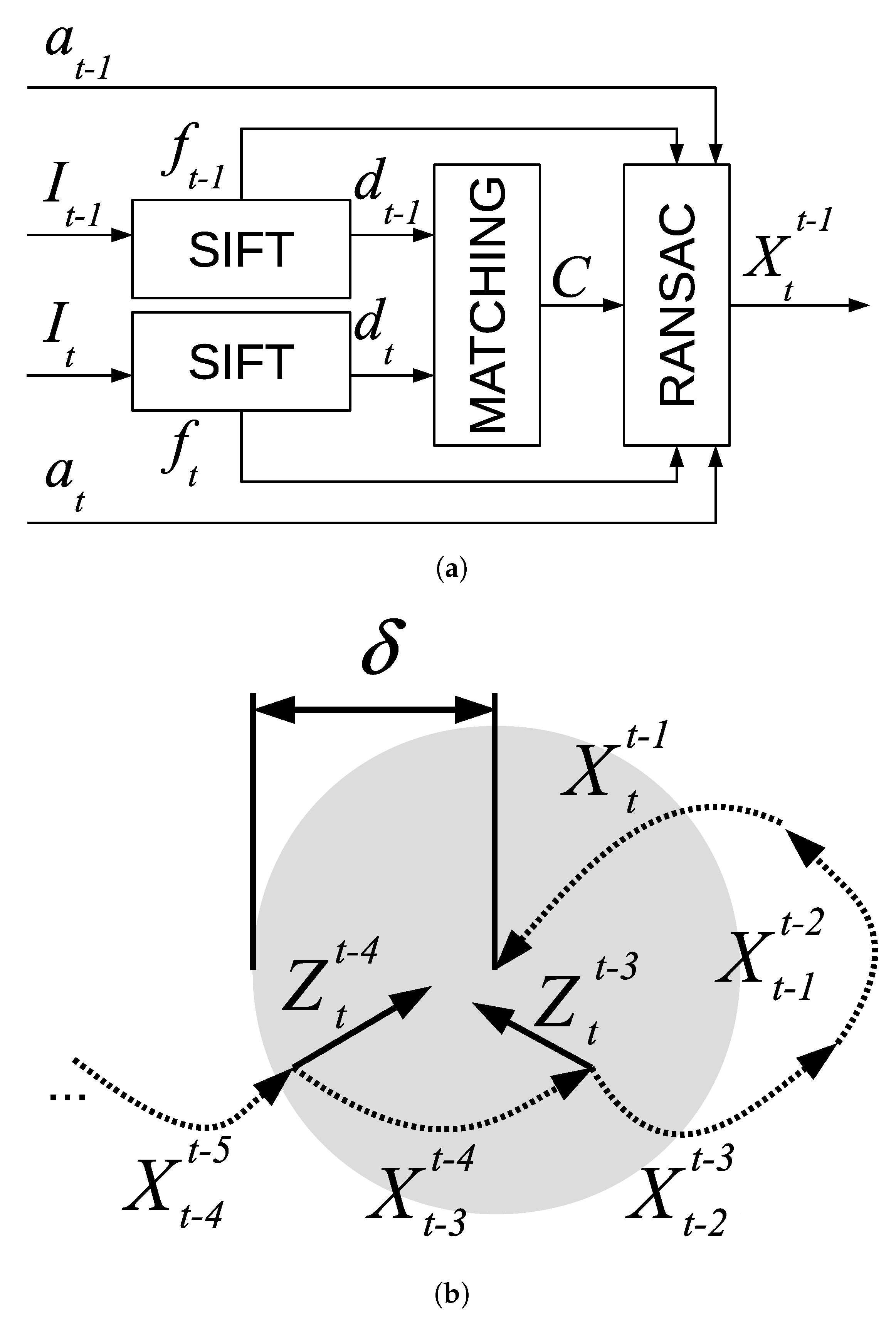
t. To achieve this goal, the following process, summarized in
Figure 3a, is used.
First, a set of SIFT features and their corresponding descriptors is computed for and . Let and denote the m and n features corresponding to images and , respectively. A feature simply represents an (x,y) coordinate within the image. Analogously, let and denote the SIFT descriptors so that each describes the feature .
The descriptors and are matched by means of standard SIFT matching. As a result, a set of feature correspondences C is obtained containing the pairs (i,j) of the matching descriptors and .
At this point, the relative motion between and could be computed by means of Equation (3) as the one that minimizes the sum of squared distances between the pairs of corresponding features.
A closed form solution to Equation (3) is available in Lu and Milios [
38]. However, since some of the existing correspondences may not be correct, our proposal is to embed Equation (3) into the RANSAC approach shown in Algorithm 1, where
is a function that converts image feature coordinates from pixel to meters.
| Algorithm 1: RANSAC approach to estimate the motion from image to image . |
 |
Roughly speaking, this algorithm is based on the idea that correct correspondences are consistent among them, thus leading to the same roto-translation, whilst incorrect correspondences are responsible for different roto-translations. Our proposal is to exploit this idea by checking if it is possible to find a consistent subset of C that is large enough to be considered correct.
The algorithm selects a random subset R of C and then computes the roto-translation X as well as the corresponding error using only this subset. These values are computed by means of Equation (3) using R instead of C.
Afterwards, each of the nonselected matchings in C is checked. If the error it introduces is below a threshold , then it is included within R. If at some point the number of items in R surpasses a threshold , the roto-translation and the error are computed again using this expanded R, and if the error is below the smallest error until now, the roto-translation is stored as a good model.
This process is iterated a fixed number of times. A description of how to compute the number of iterations depending on the expected number of inliers in the input data is provided in Fischler and Bolles [
33]. When the algorithm finishes, it is possible to recover the best roto-translation, which is a robust version of the
shown in Equation (3). This roto-translation will not be found if partial roto-translations are inconsistent and so
R never has enough items. In this case, which is unlikely to happen since consecutive images have sufficient overlap, our proposal is to use
instead.
Even though it is out of the scope of this paper, our approach to RANSAC makes it possible to properly guess (covariance of the motion estimated between and t) since it internally computes an error estimate .
6. Local Loop Detection
A local loop is a loop involving images belonging to one single session. These loops not only provide valuable information to improve each session separately but also are used to improve all the sessions together after joining them. This section is devoted to explaining how the local loops are searched.
The Local Loop Detection (LLD) is in charge of finding loop closings within one single SLAM session. First, the set of loop candidates at time step
t is built as shown in Equation (4), where
is computed by Equation (2), by searching within a predefined radius
[
6].
Afterwards, the same process to compute visual odometry described in
Section 5 is applied to image pairs
and
for all
in order to build the set of local loops
as shown in Equation (5).
In this Equation,
denotes that RANSAC did not fail to find a roto-translation between
and
.
represents the normal
so that its mean
is the roto-translation provided by RANSAC and
is the associated covariance. This covariance can either be obtained heuristically from the error computed by Algorithm 1 or using the methods described in References [
39,
40].
In general, the pose according to the trajectory
will not coincide with the pose provided by the loop closings
because of the measurement errors. The trajectory optimization described in
Section 8 is in charge of fusing both sources of information into a consistent trajectory.
Figure 3b illustrates these concepts.
7. Global Loop Detection
Global loops are those involving images belonging to different sessions, thus making it possible to establish a relation between them and to join the corresponding trajectories. Since no geometric information between two separated sessions exist, global loops have to rely on robust image matching methods. This section describes our approach to robustly detect global loops.
The goal of Global Loop Detection (GLD) is to find loop closings involving different SLAM sessions. Since in this case it is not possible to geometrically constrain the search region because there is no geometrical relation between both sessions, our proposal is to use a high performance hash-matching approach [
12] to select loop candidates and to use RANSAC to validate them.
Let the descriptor matrix
of size
contain all the
n SIFT descriptors of size
m in image
. The number of SIFT features is fixed to
n for all images. The HALOC [
12] hash (sources available in Reference [
14])
, which is a vector of which the size is
independently of the number
of features found, is built according to Equations (6) and (7) by projecting each column of
onto three different random orthogonal directions each defined by a unit vector
of
n dimensions.
The set of vectors
is defined off-line, previous to the SLAM process. The use of random and orthogonal projections avoids providing repetitive information that would reduce the hashing efficiency [
41]. Using three directions has shown to lead to an acceptable trade-off between low hash size and high performance, although other values could be used.
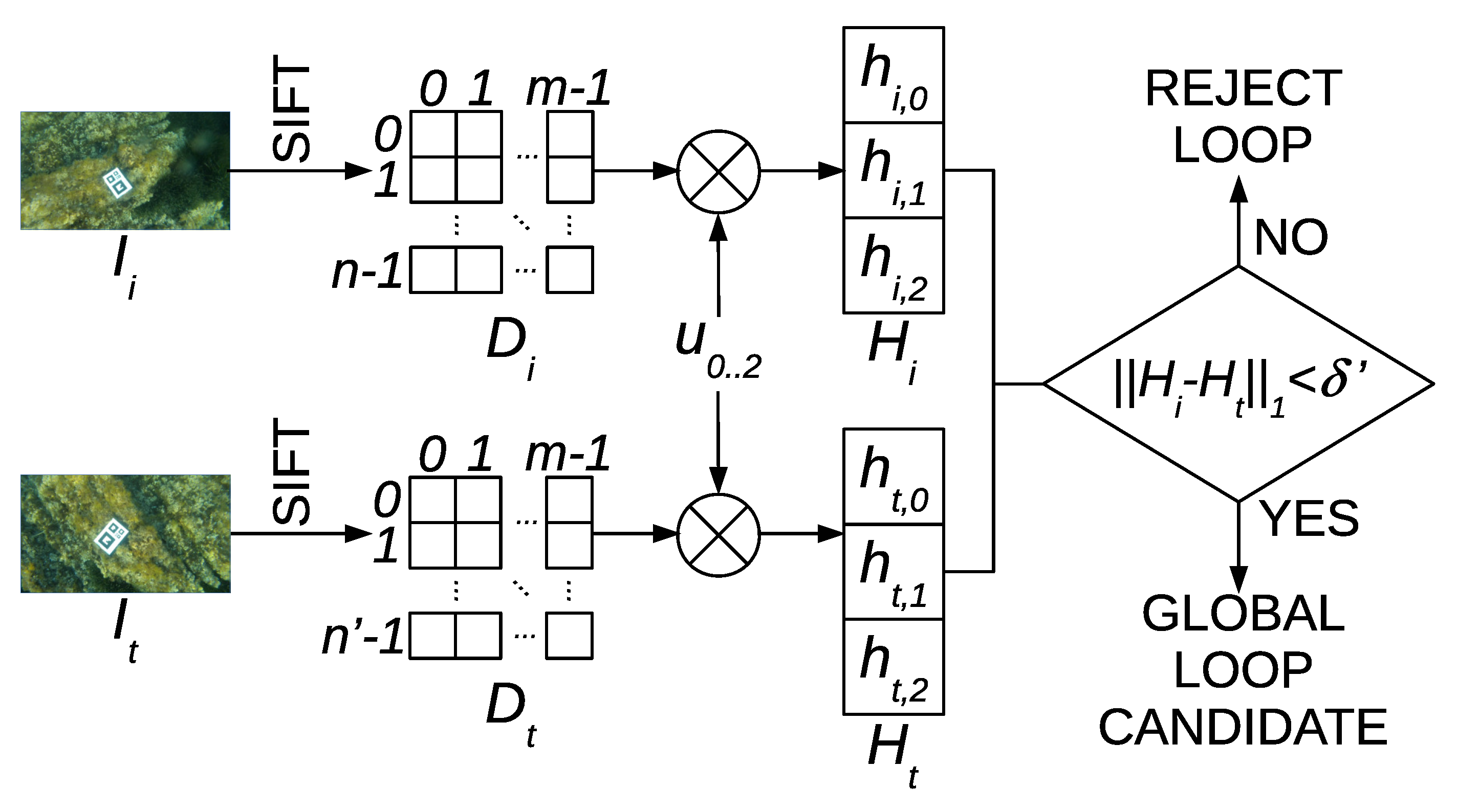
Let denote a previously gathered video sequence and be a video sequence that is currently being gathered and that will eventually capture regions overlapping with . Our proposal is to compute for every image in each sequence. This is extremely fast not only because of the simplicity of HALOC but also because the required SIFT descriptors have previously been computed to achieve odometry. Afterwards, the hash of the current image in is compared to the hash of each image in in order to build the set of candidate global loops shown in Equation (8). This is also a fast process as a comparison is performed by means of the L1 norm.
The value of
can be selected depending on the computational resources available. This process is summarized in
Figure 4. Finally, the set of global loops
is built as shown in Equation (9).
Similarly to
,
denotes that RANSAC did not fail to find a roto-translation between
and
and
is a normal of which the mean
is the transformation found by RANSAC. The corresponding covariance can be computed using the same methods proposed for the local loops in
Section 6.
8. Trajectory Optimization
This section describes how a single trajectory is optimized to meet the constraints imposed by the visual odometry and the detected local loops. As a result of this optimization, the trajectory that best explains both constraints is found. It is important to emphasize that this trajectory can also be the trajectory resulting from joining two sessions.
Let us first describe the process to iteratively build an initial guess of the trajectory by means of the odometric estimates in the current session. This is the so-called trajectory building. Afterwards, a method to optimize the trajectory using an IEKF (sources available in Reference [
15]) and the detected local loops is devised. This method, which is referred to as intra-map optimization, constitutes by itself a trajectory-based single-session SLAM approach.
8.1. Trajectory Building
The trajectory itself constitutes the state vector of the abovementioned IEKF. With each new odometric estimate , an initial guess of the trajectory is constructed according to Equations (10) and (11) by augmenting the state vector in the previous time step.
As for the initial values, following the recommendations in Castellanos et al. [
42],
and
are both set to zero so that the initial AUV pose is assumed to be a global reference frame known without uncertainty.
The covariance
of the last odometric estimate can be determined in several ways. For example, it could be heuristically estimated using the
computed by Algorithm 1. Also, the two methods presented in References [
39,
40], which rely on a solid theoretical background, can be used.
If at time t no local loops are detected, this initial guess is consolidated and becomes the trajectory itself (). If is not empty, the trajectory is optimized. This optimization is achieved by performing the IEKF update using the detected local loops as measurements. Since only loop closings can lead to changes in the stored trajectory, the state vector will not change during the IEKF prediction and, thus, it is not necessary to perform that step.
It is important to emphasize that Equation (11) alone leads to a block diagonal covariance matrix. However, the intra-map optimization will properly introduce the cross-correlation information by means of the detected local loops.
8.2. Intra-Map Optimization
Since the presence of local loops impose constraints between nonconsecutive items in the trajectory, considering the loop closings as measurements of the state vector makes it possible to optimize the trajectory. Let us model the measurement vector using the detected local loops as a normal of which the mean and covariance are shown in Equations (12) and (13), respectively.
The IEKF observation function is in charge of predicting each item in according to the state vector prior estimate . To build that function, let us first define in Equation (14) an observation function associated to each measurement in .
The overall observation function can now be constructed by means of Equation (15).
Thus, each item in is the guess, according to , of the corresponding item in . The IEKF observation matrix is the Jacobian matrix of as shown in Equations (16) and (17).
According to Equation (14), only the items from onward appear in . Thus, the partial derivatives with respect to will be zero for all , making it possible to change Equation (17) into Equation (18).
Each of these partial derivatives could be directly computed. If necessary, some approaches to express them in terms of the Jacobian matrices of the composition transformation have been proposed in Burguera et al. [
6].
At this point, an EKF update could be performed by means of
,
, and
evaluated at
. However, since
is used by the EKF to linearise
, the results would be highly influenced by such linearisation, especially when closing large loops. That is why an IEKF is used instead, since it alleviates the linearisation problems [
43]. The IEKF update iterates an EKF update relinearising the system at each iteration. The process stops after a fixed number of iterations or when convergence is achieved.
At the jth iteration, the mean and the covariance can be obtained by simply iterating the EKF. However, the computational cost can be reduced by using Equations (19) and (20). They have been obtained by operating the standard EKF formulation while taking into account the particularities of our proposal.
In these Equations, denotes evaluated at , and . The process iterates until is below a certain threshold or after a maximum number of iterations is reached. The computed mean and covariance in the last iteration constitute the optimized trajectory.
9. Map Joining
Global loops relate two different sessions and can be used to identify the geometric relationship between two sepparated trajectories. In this section, our proposal to identify such a relationship and to use it to join two trajectories into a single one is described.
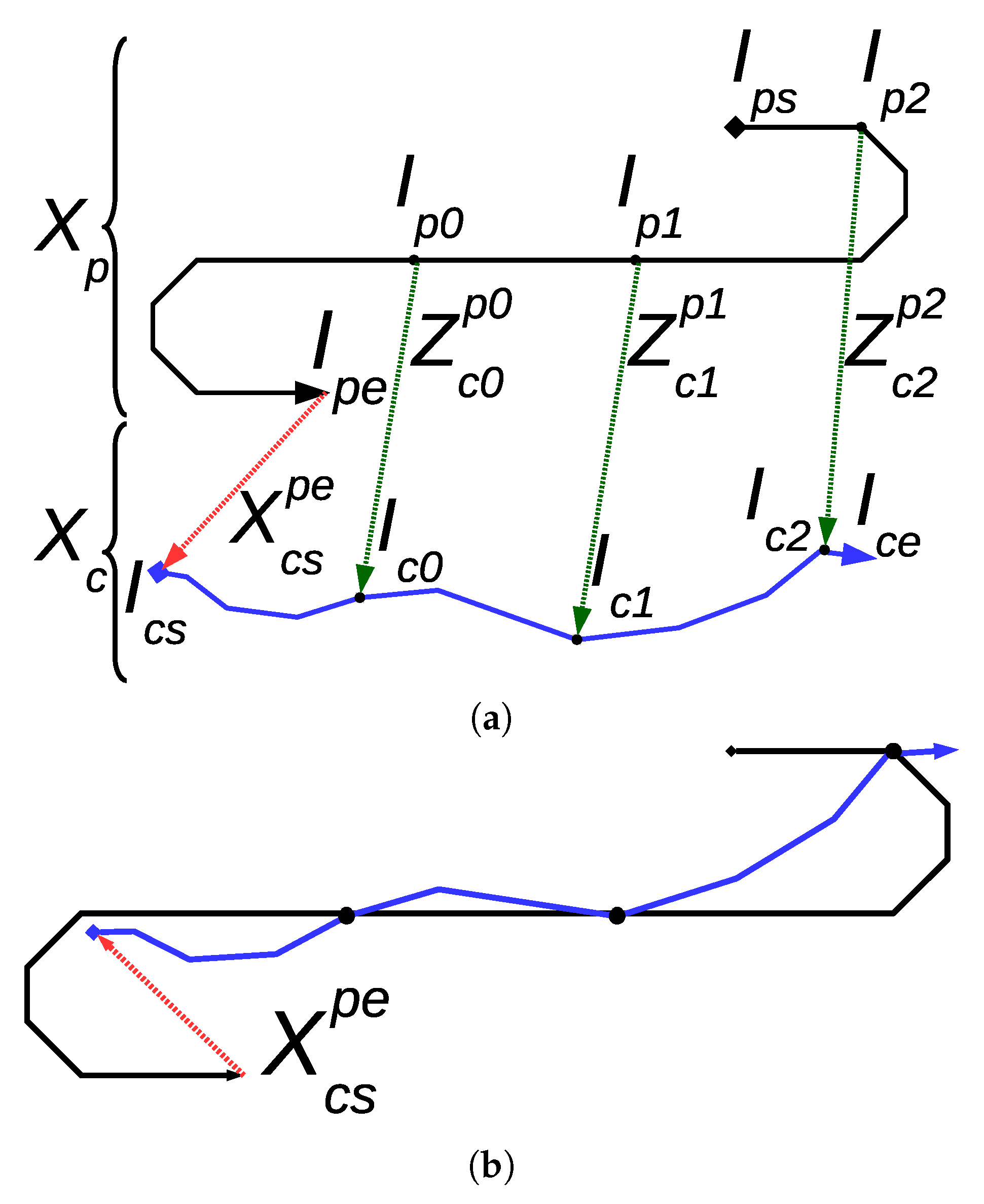
In order to preserve the trajectory structure, the goal of map joining (sources available in Reference [
16]) is to find the proper transformation between the end of the first trajectory and the start of the second one. Both trajectories, known as sessions, are separated in time, and the map joining task is aligning the current survey to a previously completed map.
Let denote the trajectory of a previous session. Let the first and last images that took part in this trajectory be referred to as and , respectively. Similarly, let denote the current session’s trajectory and let its first and last images be denoted by and , respectively. Since the map joining is performed while is being built, will be exactly .
At time step t, one or more global loops may have been found. Each of these loops relate one image in a previous session with in the current session. Our proposal is to store global loops until a fixed number K of them has been found and to then use them all to join the maps. Let , as defined in Equations (21) and (22), denote this set of K accumulated global loops.
The normals represent links between image in the previous session and image in the current one. Each belongs to (Equation (9)).
Our goal is to find the relative motion between the last image of the previous session
and the first image of the current one
. Let this relative motion be referred to as
.
Figure 5a summarizes these concepts.
This paper proposes the use of an IEKF to perform the optimization, with as the state vector and as the measurement. That is, the IEKF will find the that better explains all the loop closures. Since only depends on the loop closings, which constitute the measurements during the IEKF update, there is no need to perform the IEKF prediction.
Let us begin by building the observation function (Equation (23)) which provides an estimate of each loop in from the state vector.
Each estimates the loop , with as the transformation from the loop closing image to the last image of the previous session and as the transformation from the first image in the second session and the loop closing image . Both can be computed by means of Equation (2).
The Jacobian matrix of the observation function, which is needed by the IEKF optimization, can be computed as shown in Equations (24)–(28). The terms s and c denote sin and cos, respectively.
Now, the IEKF in Equations (19) and (20) can be applied to find the transformation between both maps. The standard formulation is provided next only for clarity purposes. At the jth iteration of the IEKF, the mean and the covariance of the state vector can be computed by means of Equations (29)–(31). The term denotes evaluated at .
The process is iterated until is below a certain threshold or a maximum number of iterations is reached. When that happens, the final and constitute the outputs and of the IEKF.
being the initial guess of the state vector, our proposal is to compute it from one of the loops in , since there is a single solution in the presence of a single loop and, thus, a closed form expression exists. Equation (32) shows such a closed form expression if the first loop is used.
Since expresses a transformation between the end of the previous session and the beginning of the current one, it is extremely simple to use it to join both sessions into a single one. Equations (33) and (34) show the mean and the covariance of the joined trajectory , where and denote the covariances of and , respectively.
In this way, the resulting trajectory is consistent with both sessions and can be used, from this moment onward, to perform the single-session SLAM described in
Section 8.
Additionally, with our proposal being able to simultaneously take into account several global loop closures, different sessions may be kept separated until necessary, reducing the computational cost. Also, the adopted trajectory-based structure with links between different sessions allows to easily separate joined maps whenever is necessary for the sake of computation time.
Figure 5b shows the resulting trajectory after applying the described process to the example in
Figure 5a.
The whole process is summarized in Algorithm 2. The function compute_tails is in charge of computing the motion from one of the loop closing images to the end of the previous session and from the beginning of the current session to the other loop closing image. As stated previously, this is achieved using Equation (2). The function compute_observation computes each of the (see Equation (23)) and the corresponding Jacobian matrices (Equations (24)–(28)). Finally, IEKF_update refers to Equations (29)–(31).
| Algorithm 2: Map joining. |
 |
As can be observed, the algorithm begins by computing an initial estimate using the first existing loop in according to Equation (32). Afterwards, in each IEKF loop, the observation function as well as its Jacobian matrix are iteratively computed by appending a new term for every measurement in . Finally, when the algorithm converges, the joined trajectory is built by linking and using the obtained .
10. Experimental Results
This section presents an extensive set of experiments evaluating the main building blocks of our proposal. These experiments, which have been conducted using real data gathered in coastal areas of Mallorca (Spain) colonized with Posidonia oceanica, assess both qualitatively and quantitatively the ability of our proposal to properly perform multi-session SLAM.
10.1. Experimental Setup
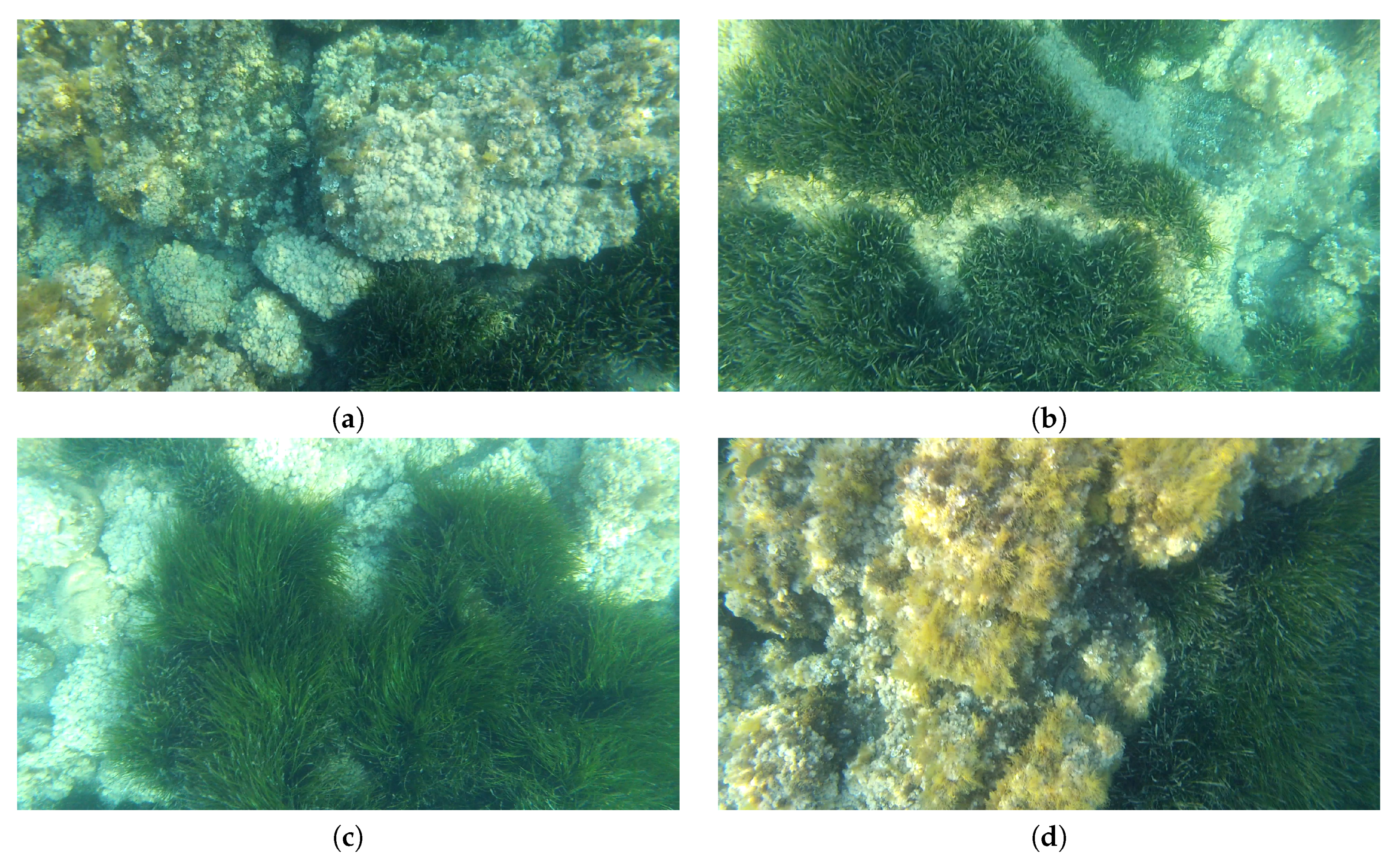
For a first evaluation, two different, partially overlapping video sequences and were recorded in Port de Valldemossa (Spain) with a bottom-looking camera in a marine environment with sand, rocks, seagrass, and moss. The camera was attached to a diver with the lens axis approximately perpendicular to the bottom. The diver moved on the water surface in an area with an approximate constant depth of 3 m. The lack of any other sensorial data which could be supplied by an AUV makes the localization system a pure vision-based approach.
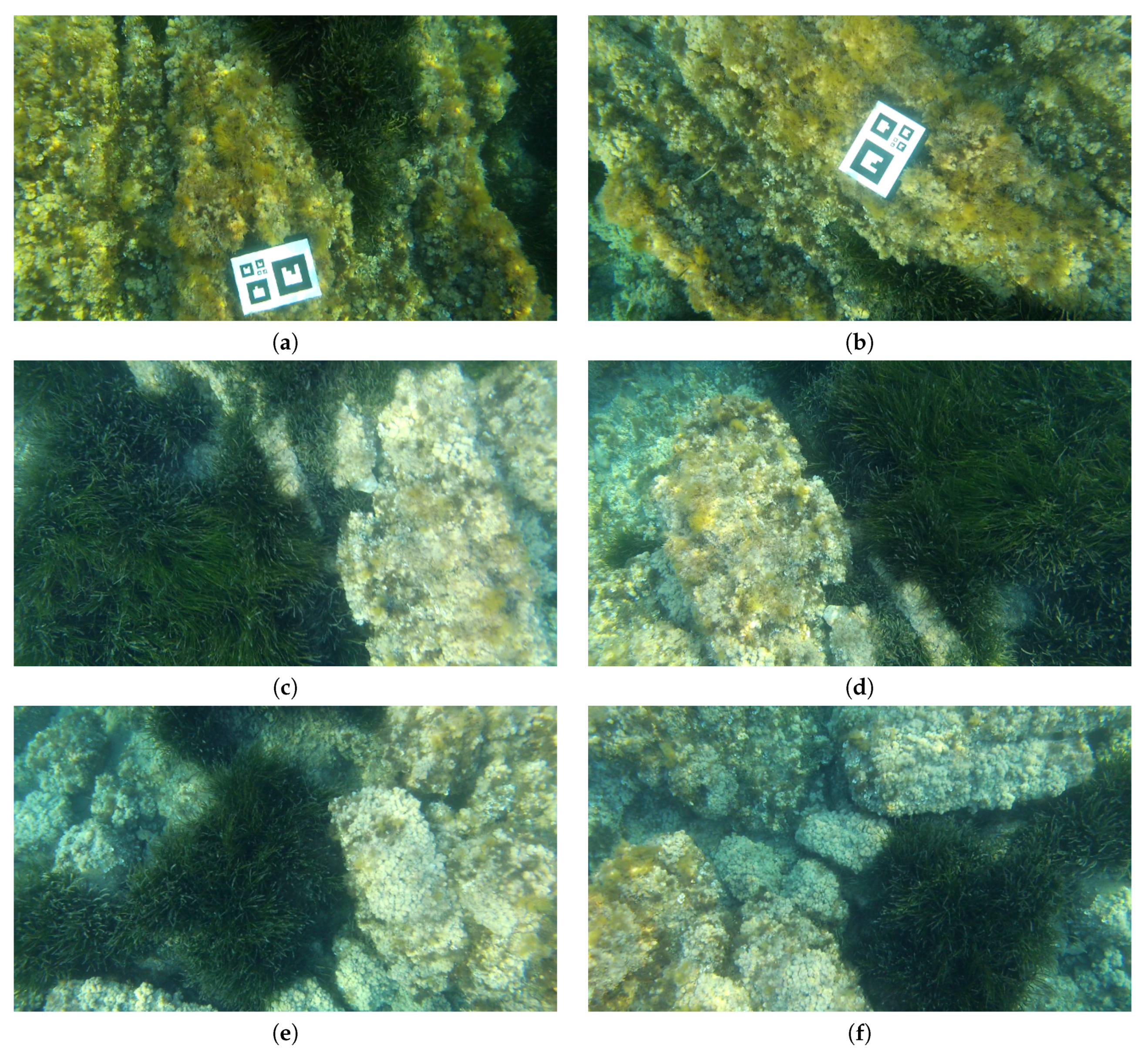
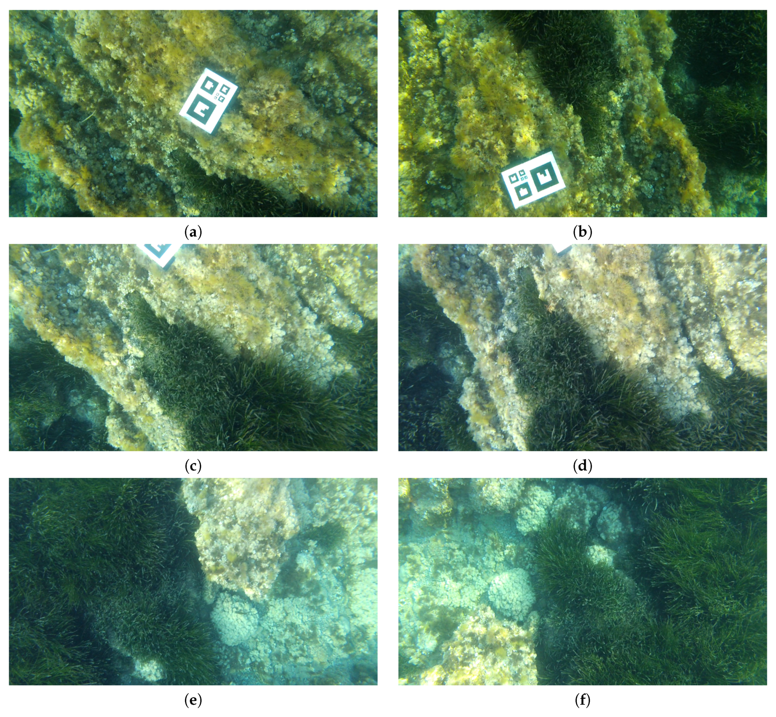
Some images of these sequences are shown in
Figure 6, where it can be observed that the region is populated with Posidonia oceanica, a seagrass that forms dense colonies characterized by its long and thin leafs. Posidonia is crucial in the maintenance of the Mediterranean marine ecosystems and declared by the European Community a species with special protection. One of the tasks in the ARSEA project includes mapping Posidonia meadows and quantifying their bottom coverage using an AUV and several algorithms to discriminate the Posidonia from the background based on deep learning [
44]. Due to the particular texture of the Posidonia and the slight motion of its leafs caused by the water current, tracking stable visual features in consecutive overlapping frames is a challenging task. A high number of outliers and/or a slow feature detection process, matching, or tracking might compromise the accuracy in the calculation of the visual odometry and the registration of images that close loops. However, previous references [
45,
46] already showed that SIFT is one of the best features to be used in this type of underwater environments in terms of matching and tracking performance. SIFT is also the key feature type in HALOC. Although processing SIFT is slower than other descriptors, the C++ version of HALOC is highly efficient in areas with Posidonia [
12,
35]. In our opinion and according to our experience and obtained results, given the robustness and traceability of SIFT, spending an additional slight portion of time in the process of RANSAC-based feature detection and matching to obtain more reliable trajectories is more preferable than using other simpler features that present less computational cost than SIFT (thus faster) but can cause larger inaccuracies in the image transformations because they also give a higher number of outliers when tracked/matched.
The camera altitude was computed at the beginning of each video sequence by means of a static visual marker of known size, placed at the sea bottom. This marker served as the origin and end point of both trajectories. From the sequence, 226 key images were extracted, and 199 were extracted from .
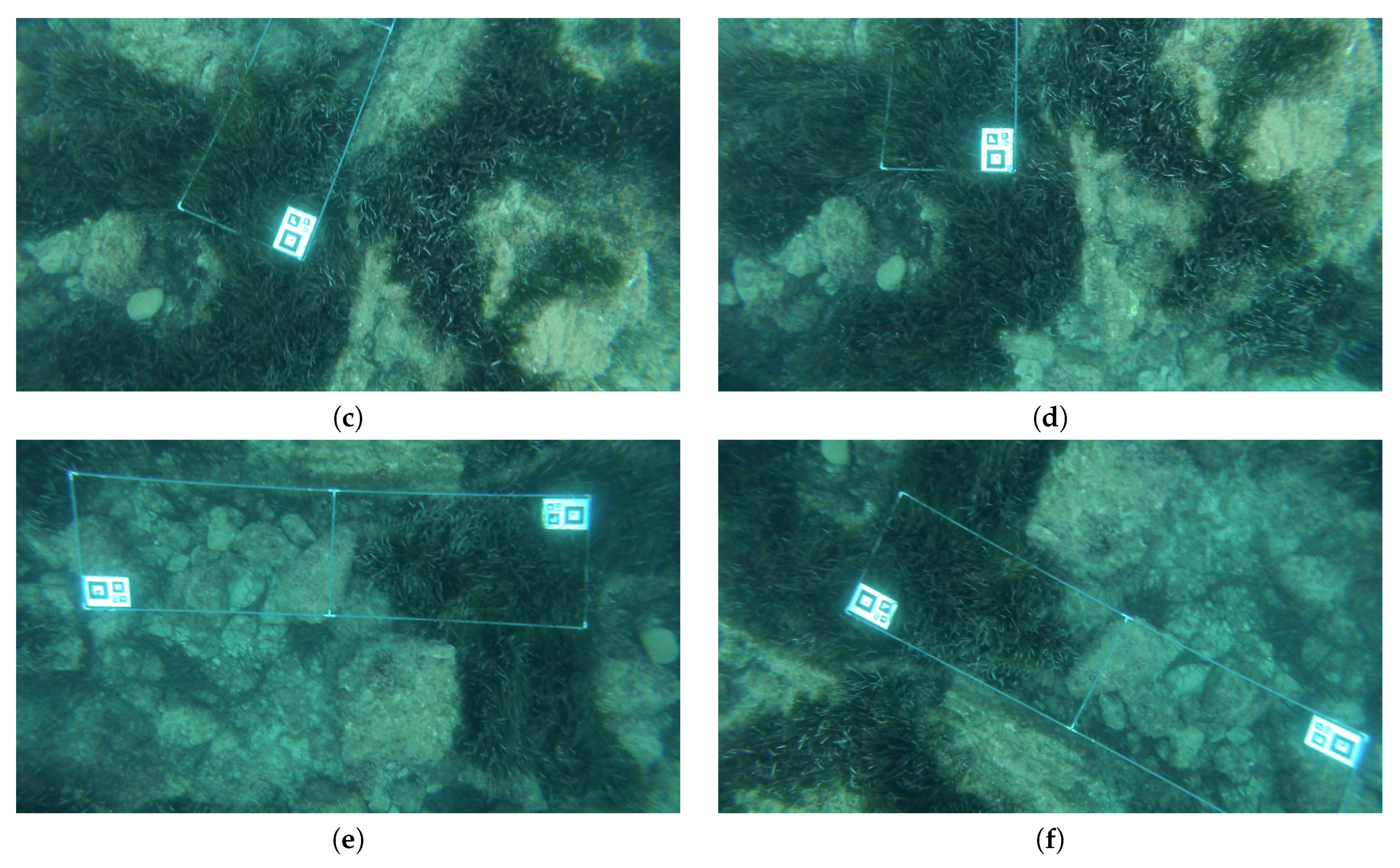
A second pair of trajectories, and , were recorded also by a diver in Port de Valldemossa far from and but using the same infrastructure as described above and navigating on the water surface at an approximate constant altitude of 4 m. In this case, the initial altitude was computed thanks to a static structure of known dimensions formed by markers and plastic tubes placed at the sea floor. A total of 209 key frames were selected, the first 152 corresponding to and the next 57 corresponding to .
and also started and finished over one of the static markers forming the structure. Once this structure was deployed, it was not touched until and were grabbed. For all sequences, the altitude was assumed to be constant during each session and the video resolution was 1920 × 1080 pixels, grabbed at 30 frames per second, and prior to their use, all images were scaled down to 320 × 180 pixels.
Finally, a third pair of video sequences, namely
and
, were recorded by the SPARUS II AUV [
47] property of the University of the Balearic Islands, moving at a programmed constant altitude of 3 m in an area of 16 m depth. The altitude of the robot is well known and obtained from its navigation filter which integrates the DVL, an Inertial Measurement Unit (IMU), a pressure sensor, an Ultra Short Baseline (USBL) localizer, and a stereo 3-D odometer [
48]. The aim of these video sequences is to test our proposal in larger environments with complex imagery due to the massive presence of Posidonia on the sea bottom. In particular,
was obtained along a trajectory of 93 m and
involved a 114-m mission. While gathering
, the AUV was programmed to perform a rectangular loop of 20 × 15 m. As for
, the AUV mission was to perform two smaller loops on one side of
.
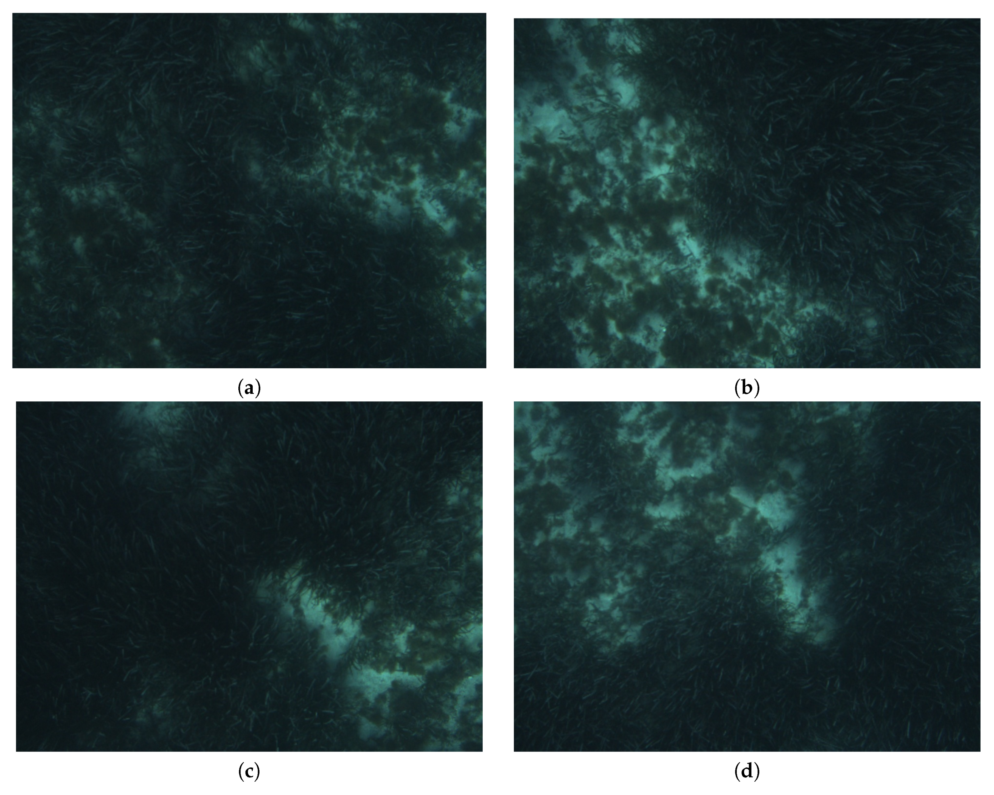
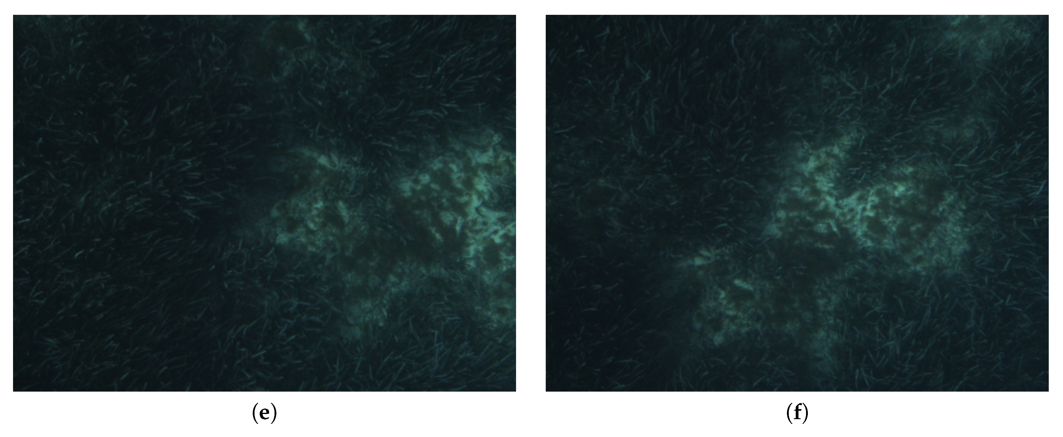
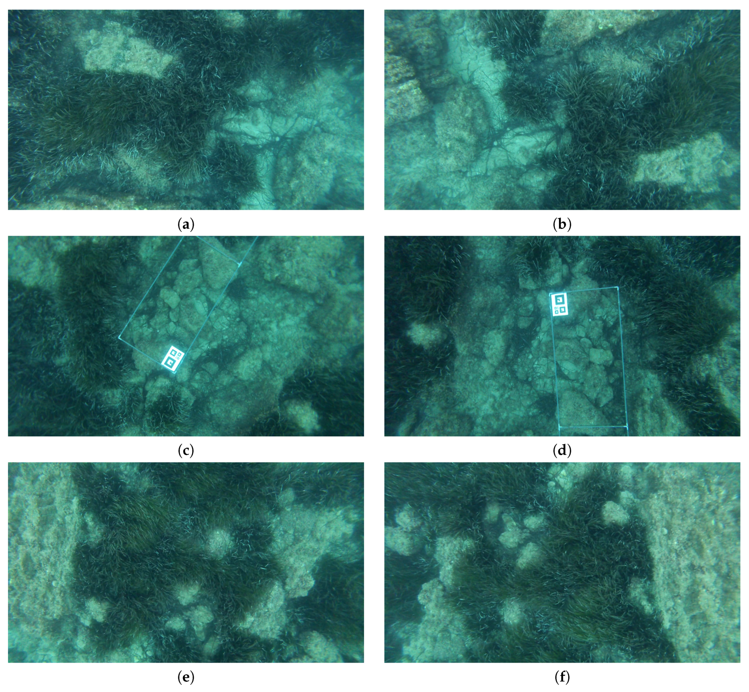
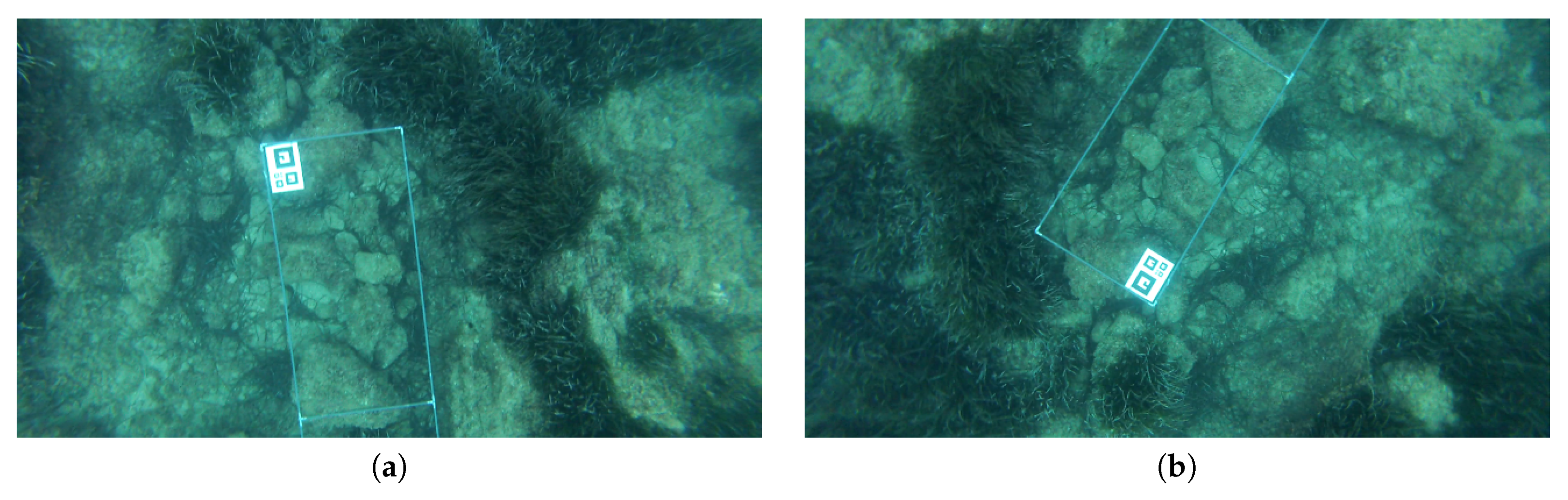
Figure 7 shows some images extracted from
and
. As it can be observed, illumination was deficient, resulting in dark images with low contrast. In these types of environments, the altitude parameter is extremely important. Cameras at larger altitudes will provide wider fields of view and, thus, the possibility to find more loop closings, but conversely, if the illumination conditions are not optimal, especially at larger depths, the feature matching process can decrease its performance and affect directly the accuracy of the visual odometry calculation and the loop closing detection. In our environments and with our robot and its equipment, altitudes between 3 and 5 m give a good trade-off between image overlap and illumination conditions. A total of 400 key images were extracted, 200 belonging to
and 200 bwlonging to
. In all these image sets, the Posidonia appears as the darker and/or greener areas, being the clearer areas such as stones, pebbles, or sand in the background.
Given the extreme difficulty to obtain a ground truth trajectory in underwater environments without a Long Baseline (LBL) positioning infrastructure and specifically in medium or large areas colonized with seagrass, the assessment of the map-joining system has been done not from a vehicle factual ascertainable motion data but by obtaining, (a) on the one side, a qualified mosaic to provide visual evidences of correctness and, (b) on the other side and for the sake of a quantitative evaluation, the difference between a set of 2-D transformations (
-(x, y and yaw)) between image pairs that close local and inter-session loops obtained according to the estimated trajectories and the same 2-D transformations
obtained manually with Matlab (transformation ground truth) (see
Section 10.3 and
Section 10.4).
10.2. Loop Closure Detection
Similarly to Ozog and Eustice [
30], the consistency of a SLAM approach is now partially measured quantitatively by counting the number of visual loop closures and then through the derived parameters of precision, recall, and accuracy.
A total of 13 image pairs (11 in V1 and 2 in V2) were retrieved as single-session loop closings, using feature matching and RANSAC as described in
Section 6 around a region surrounding the current image, resulting all true positives (TP). In order to assess the global loop detection using the signature method, all images of both video sequences
and
were hashed using HALOC. Equation (8) was applied by means of relating every key image (query image) of
with the 5 images (so-called candidates) of
that presented the lowest difference in terms of L1-norm between the hash of the query and the candidate. After this, all these preselected image pairs that presented a number of inliers (SIFT feature matching with RANSAC) higher than 25 were confirmed as loop closings. This threshold was set experimentally, since all the real (single and multi-session) loop closings presented more that 25 inliers and the overwhelmingly majority of image pairs that did not close loops had less than 10. However, this threshold needs to be set as a function of the observed environment. Thirty-five image pair candidates to close global loops (between
and
) were found, from which 34 were TP and 1 false positive (FP), resulting in a precision, defined as
, of 0.97.
Four hundred and twenty-five image pairs were labeled as non-loop closings, including local and global, and verified by visual inspection. Four hundred and two were true negatives (TN) (images that really did not close loops), and 23 turned out to be false negatives (FN) (loop closings classified as non-loop closings). The recall defined as was 0.7927, and the accuracy defined as was 0.9533.
In summary, although some real loop closings are missed in the detection process (implicit in a recall slightly lower than a 80%), the percentage of true loop closings detected (single and multi-session) with respect to the total of loop closings finally proposed is close to 100%.
Figure 8 shows a sample of 3 pairs of single-session loop closings located in both image sequences
and
. Dark areas correspond to Posidonia while clear areas correspond to stones and pebbles.
Figure 9 shows a sample of 3 pairs of multi-session loop closings between the two image sequences. Again, dark areas show the Posidonia and clearer areas correspond to stones and pebbles.
An evaluation on and was done following exactly the same procedure used with and to retrieve all local and global loop closings. The feature matching threshold was also set to 25. Four hundred image pairs were labeled as negatives (no loop closings), and 130 were labeled as TP loop closings, 21 were labeled as multi-session, and 109 were labeled as single session, giving a precision of 1. The evaluation of these results was also done by visual inspection. From the 400 negatives, 349 were TN and 51 turned out to be FN. The recall result was 0.72, and the accuracy was 0.9. With a threshold of 25, some real loop closings are missed. However, a 100% in precision means that all loop closings that will be used in the SLAM process are true.
Figure 10 shows a sample of 3 pairs of single-session loop closings located in both image sequences
and
. Dark areas again correspond to Posidonia.
Figure 11 shows a sample of 3 pairs of multi-session loop closings between the two image sequences
and
.
A similar evaluation was performed with
and
. In this case, a total of 59 loops between both sessions was found.
Figure 7 shows some examples. The images in the left and right columns belong to
and
, respectively. As it can be observed due to the kind of imagery that loops are hard to detect by simple visual inspection. Thus, these video sequences clearly show the loop detection capabilities of HALOC in these type of environments.
10.3. Multi-Session SLAM
In order to quantitatively evaluate our proposal, we have selected five image pairs of each video sequence that close a large local loop. By large local loop, we mean that the first and the second image in each pair overlap but that, between the times at which these images were gathered, the camera field of view did not overlap any of them for at least 40 s. Actually, this time surpasses two minutes in five of the ten image pairs and three minutes in two of them.
For each of these image pairs, we have computed manually the exact pose of one image with respect to the other, building two sets of local ground truth, and , defined as and , which include the relative poses between images. Similarly, we have selected five image pairs that close global loops, computing the exact pose of the second image in each pair with respect to the first one, building a global ground truth.
Thereafter, let us define the error as the average distance between the relative positions according to the ground truth and the corresponding relative positions according to the estimated trajectory as shown in Equation (35). In this Equation, denotes the relative position of image j with respect to image i according to the trajectory being evaluated.
Overall, the quality of the vehicle pose estimated by the odometry, the single-session SLAM within the first () and second video sequences () and between both video sequences (multi-session SLAM) can be computed.
Figure 12 and
Figure 13 depict the trajectories for
and
. In these figures, SLAM refers to each single-session separately and MSLAM denotes the multi-session SLAM. The number after MSLAM states the number of global loops used to join the maps. That is, the number refers to
K in Equations (21) and (22). Therefore, MSLAM1 corresponds to joining the maps after the first global loop was detected. MSLAM10, MSLAM20, and MSLAM30 delay the map joining until 10, 20, and 30 global loops were found, respectively.
Table 1 summarizes the obtained quantitative results. The time consumption has been measured in seconds on a Matlab implementation executed in a standard laptop (i7 CPU at 3.1GHz using a single core) running Ubuntu 16.04LTS. The odometry error is expressed in meters, and it is reasonably low during the first session but increases considerably in the second one. Thus, SLAM (either single-session and multi-session) provided a slight improvement to the first session but a very large improvement during the second one. It can also be observed that the results corresponding to each session are similar if we compare the single-session approach to the multi-session one.
The different delays to join the maps (10, 20, and 30) barely affect the quality of the final estimates since errors are almost constant. To the contrary, the execution time is reduced to 78% if the maps are joined when 30 loops are detected instead of joining them with the first loop. Thus, delaying loop closure is responsible for a large reduction in time consumption.
In the Matlab implementation, the CPU usage was, on average, 24.3% for the odometry, 62.4% for the single-session SLAM, and 90.5% for the MSLAM30 map joining procedure. A CPU usage far below these percentages can be expected with an optimized C++ code instead of Matlab. Although out of the scope of this paper, it is worth mentioning that a C++ implementation is currently being developed by the signing authors under the ROS middleware [
49] to be installed in our AUV and to be run online during the missions. Additionally, given the high speed at which the C++ implementation of HALOC is able to propose loop closing candidates [
12], the use of the whole system on-line, in our view, is perfectly feasible. Nonetheless, a further complete assessment will be necessary.
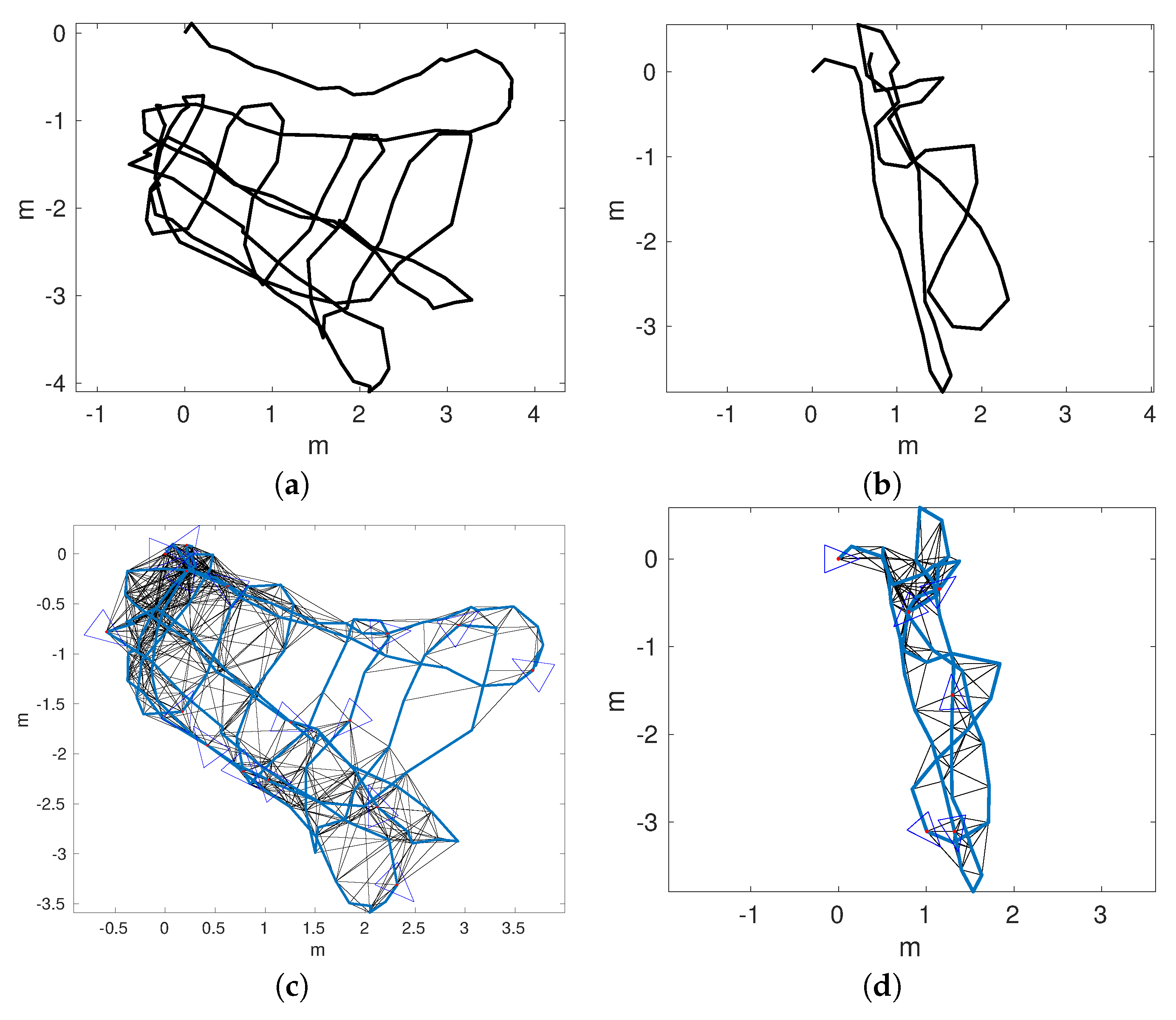
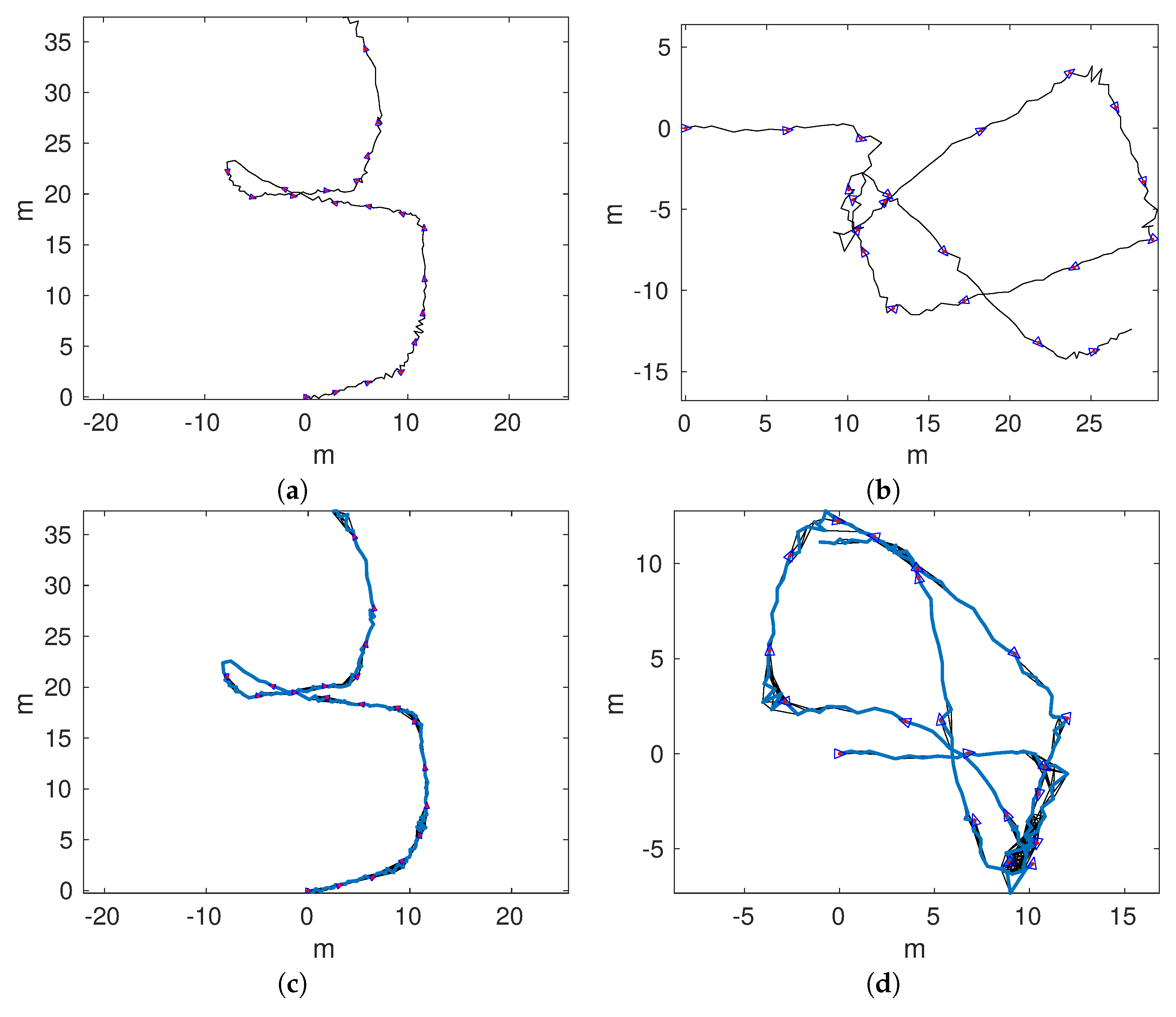
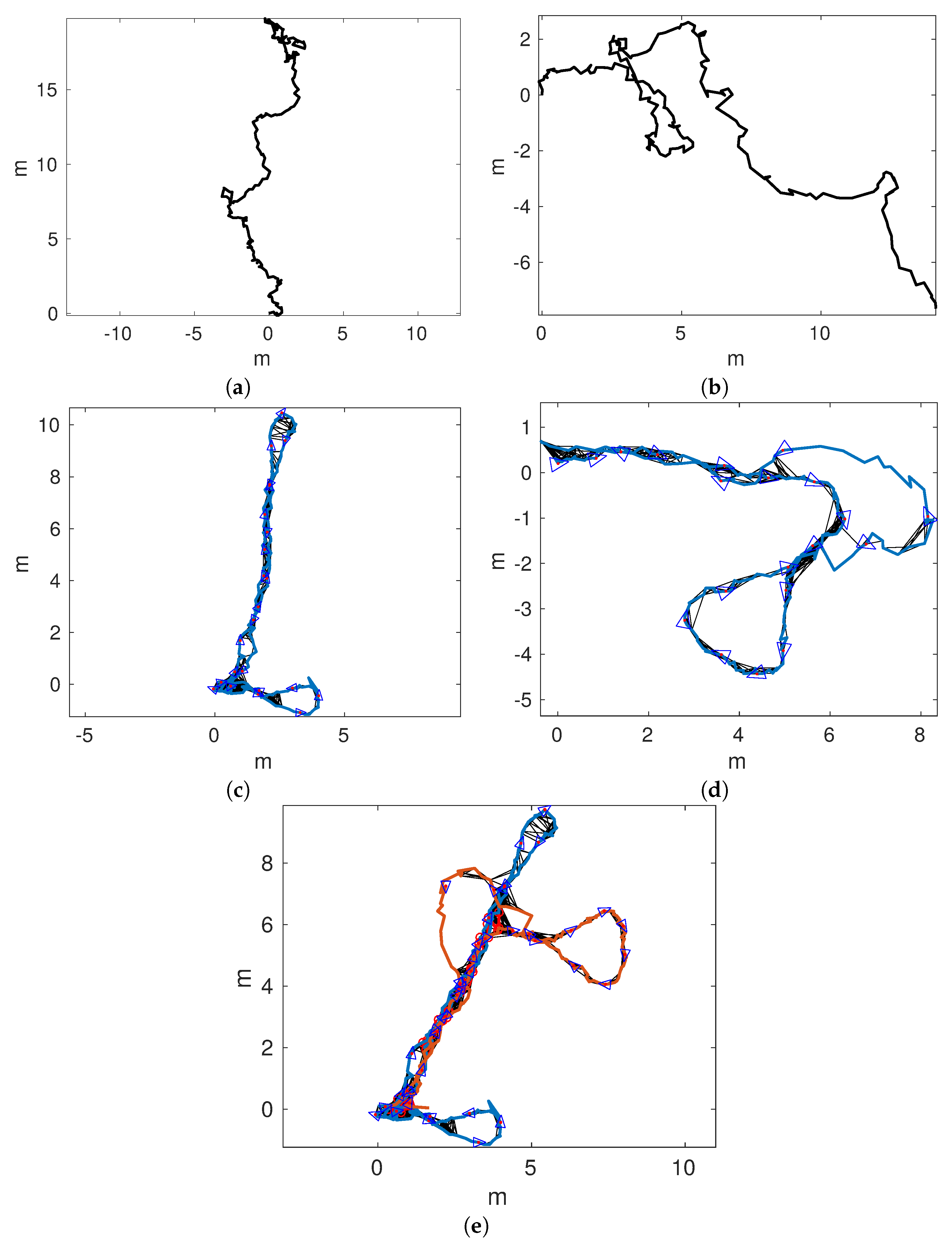
Figure 14a,b shows the odometric trajectories of
and
, respectively.
Figure 14c,d depicts the local SLAM trajectories of
and
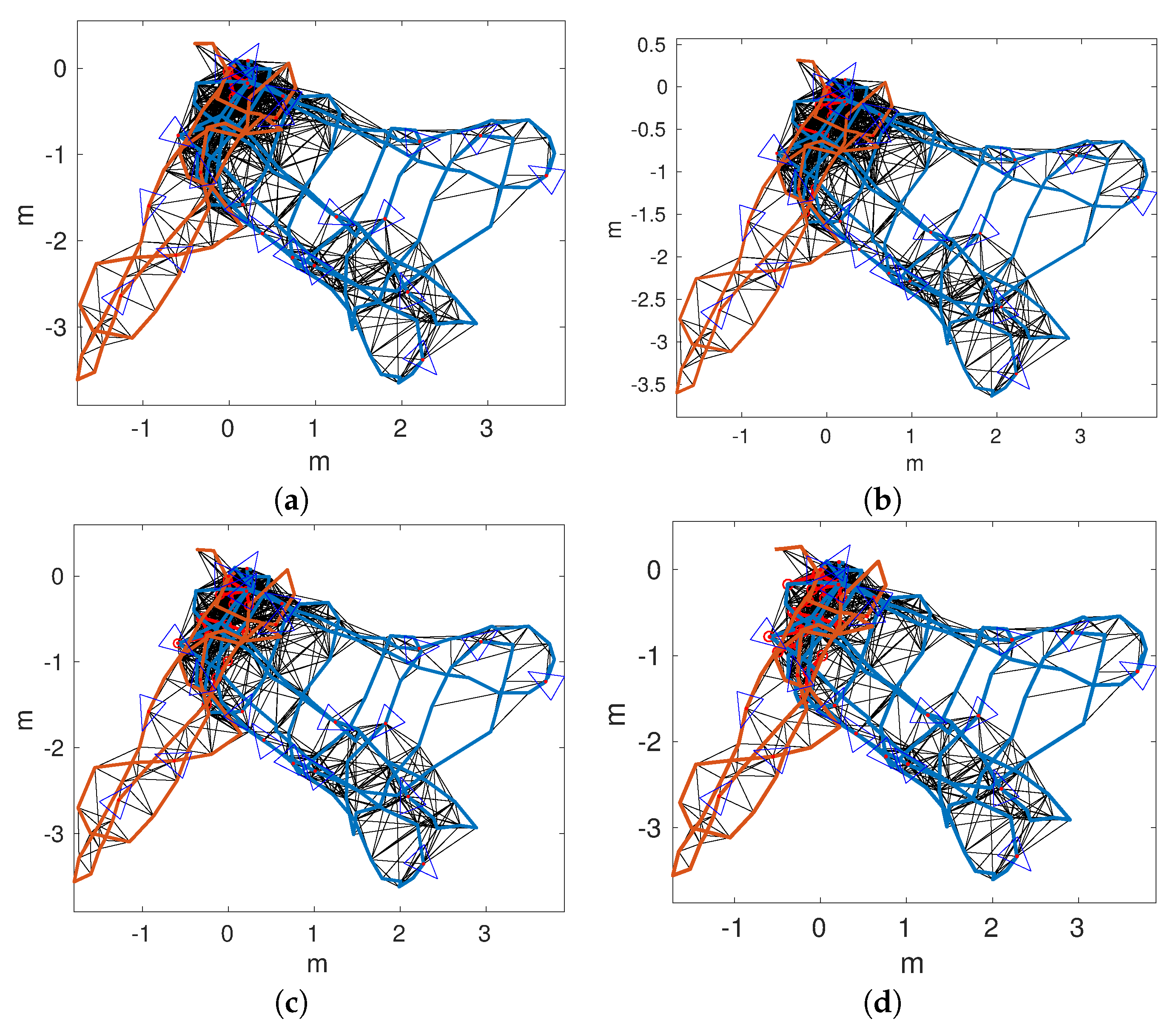
, respectively. Finally,
Figure 15a–d shows the connected maps, delaying the joining step until 1, 5, 10, and 15 loop closings were detected. Since both sequences started and finished over the structure, it is easy to see that the odometry drifts at the end of
and, to a lesser extend, in
.
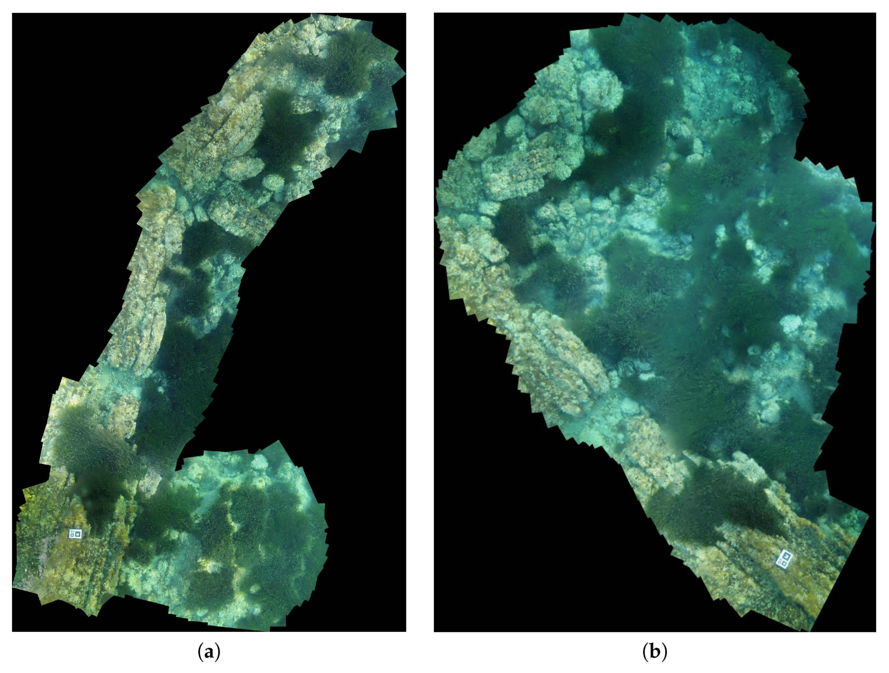
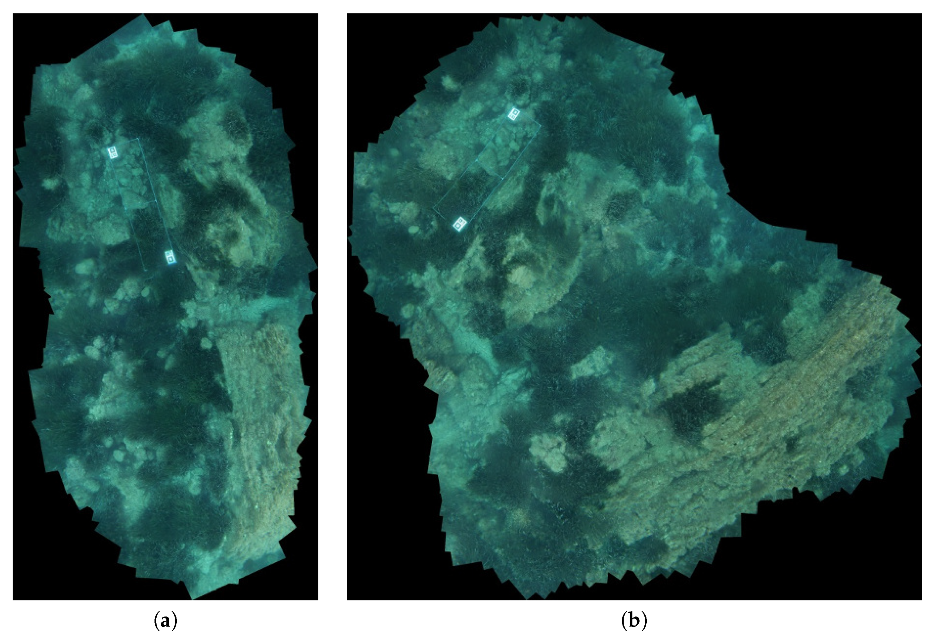
Figure 16 and
Figure 17 show four photo-mosaics corresponding to sequences
,
,
, and
, included for the sake of an easy and fast visual qualitative evaluation of the joined trajectories. Both mosaics were built with the same key frames used in the SLAM processes and
Binary descriptor-based Image Mosaicing (BIMOS) [
50]. BIMOS-related references [
50,
51,
52] already showed the good performance of this mosaic approach in terms of accuracy and execution time and of application in underwater environments with seagrass (see Bonin-Font et al. [
51]). Consequently, its assessment is out of the scope of this paper.
The marker visible on mosaics corresponding to and indicate the start and end of both trajectories. The relative position of the mosaics correspond to - and - with respect the single marker in the formers, and the structure in the later coincide very closely with the form of the resulting joined maps.
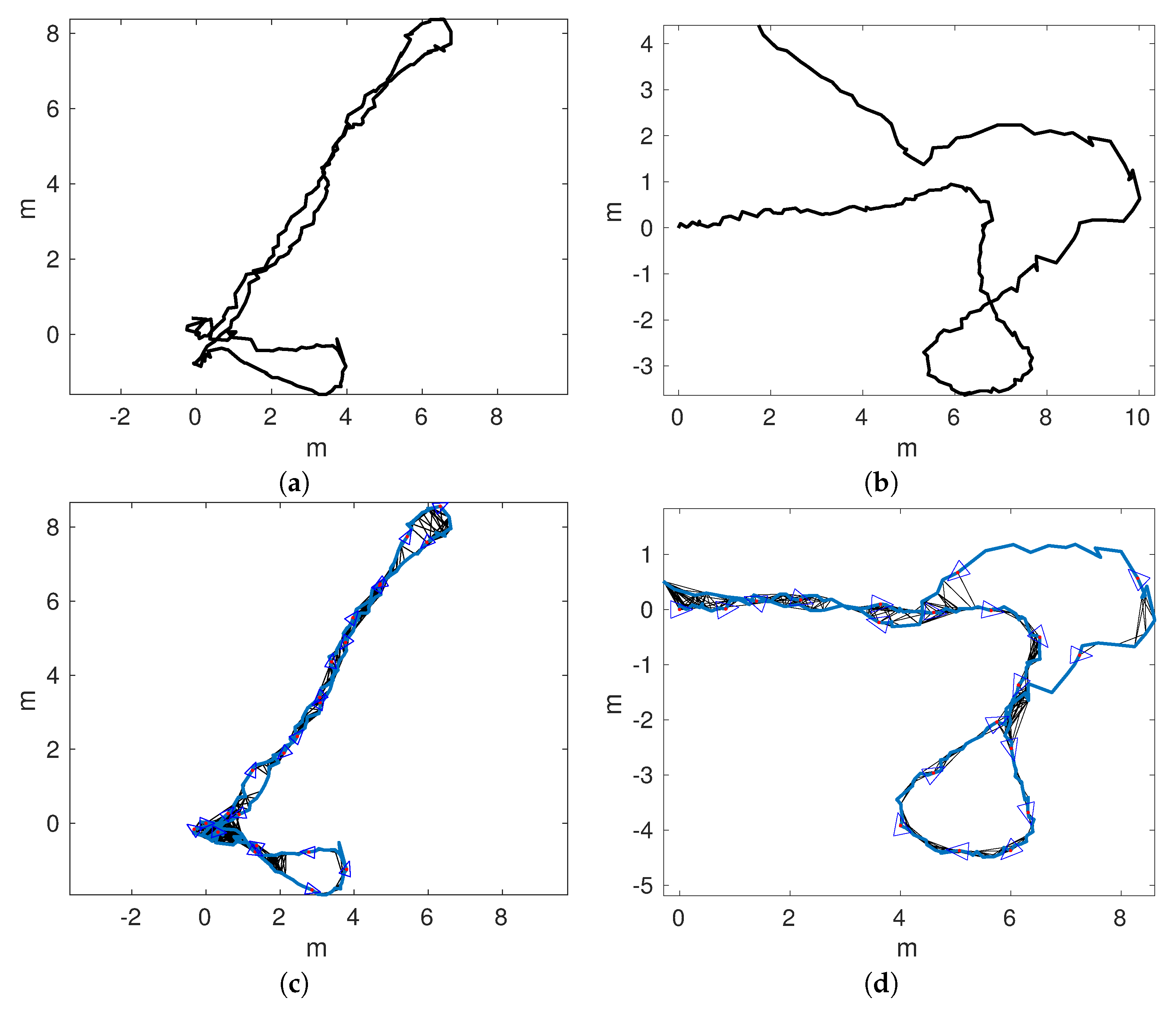
A final experiment has been performed, aimed at showing the quality of our proposal in front of larger trajectories and bad illumination conditions. To this end, and have been used.
Figure 18 shows the obtained trajectories. In particular,
Figure 18a,b shows the trajectories according to pure visual odometry. In both cases, significant odometric errors lead to trajectories that barely resemble the actual mission performed by the AUV.
Figure 18c,d shows the trajectories obtained by single session SLAM. In this case,
was substantially corrected. However,
remains almost unchanged with respect to pure odometry. In this case, the odometric error was so large that the geometric constrains prevented the detection of relevant loops.
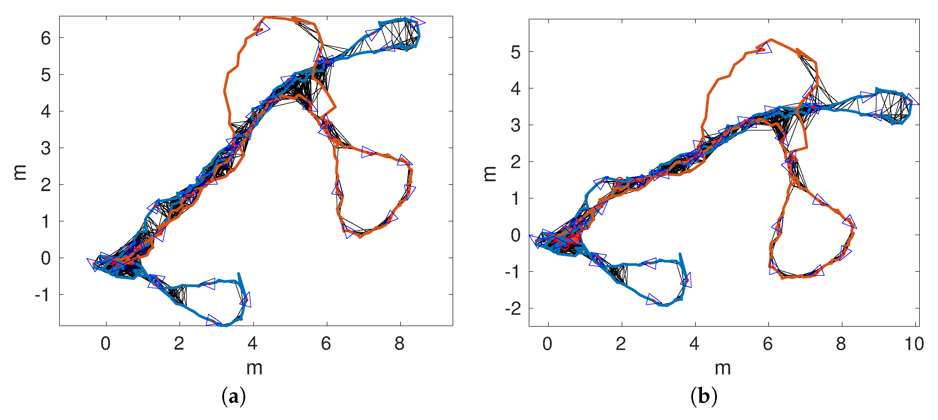
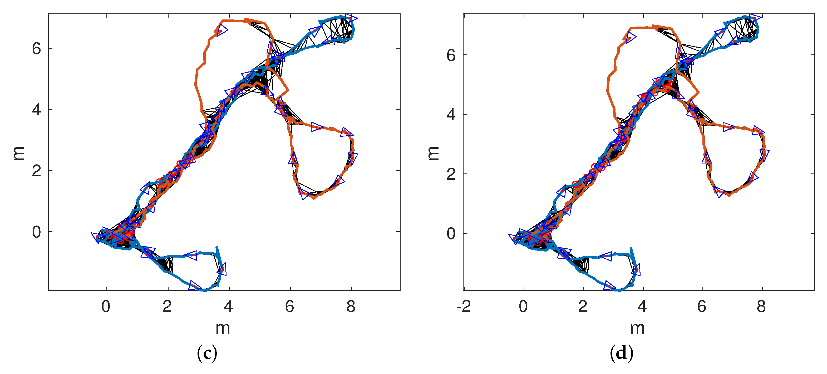
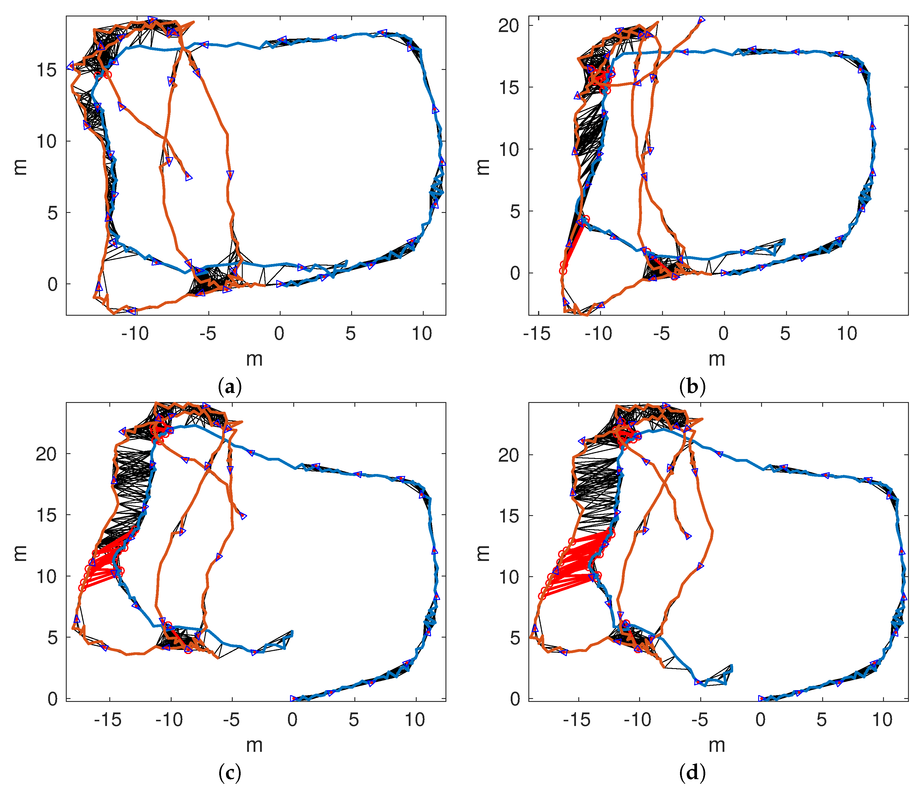
Figure 19a,d shows the trajectories according to multi-session SLAM if maps are joined after detecting 1, 10, 20, or 30 global loops. As can be observed, in all cases, the overall structure of
is recovered, thus leading to a large improvement with respect to single session SLAM.
It can also be observed that the larger the delay to join the trajectories, the worse is the result. For example, for MSLAM20 and MSLAM30, the loops involving the start and the end of have not been detected. This decrease of the quality with the delay is reasonable and consistent with previous results: as the delay increases, less local loops are available to improve the joined trajectory.
Table 2 shows the execution times. As can be observed, the multi-session execution time is significantly larger that of single session SLAM. This is mainly due to the fact that few local loops are detected in single session SLAM, especially in
. These results also show that the larger the delay to join the trajectories, the lower the execution time. For example, switching from a delay of one to a delay of 30 leads to a reduction of 38.57% of the execution time.
10.4. Robustness
In order to test the robustness of our proposal, we have corrupted the odometric estimates of and with five different levels of additive zero mean Gaussian noise. The two sigma bounds of these noises ranged from 5 cm in x and y and 5 in orientation for noise level 1 to 25 cm in x and y and 25 in orientation for noise level 5.
Each corrupted odometry has been used to perform single and multi-session SLAM with different loop-closing delays.
MSLAM1, MSLAM10, MSLAM20, and MSLAM30 denote that the maps were joined after detecting 1, 10, 20, and 30 global loops, respectively. The local and the global errors have been recorded in each case. This experiment has been repeated 60 times for each noise level.
Table 3 summarizes the obtained results by showing the mean (
) and the standard deviations (
) of the obtained errors for each noise level (N.). MSSession denotes the multi-session SLAM. All values are expressed in meters.
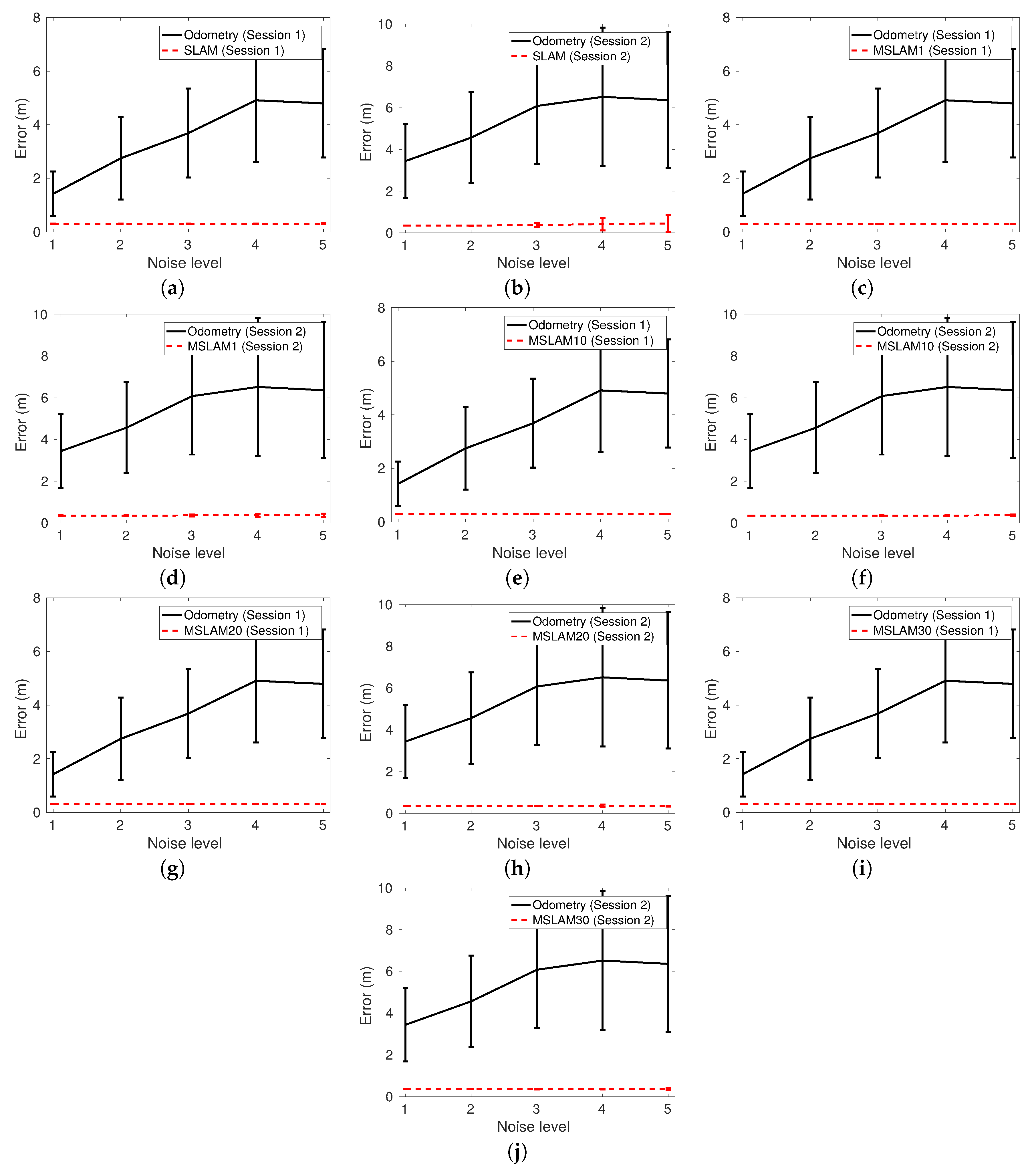
Figure 20 compares the errors of each tested SLAM approach to those of odometry as a function of the noise level. Firstly, both SLAM errors, single and multi-session, are always below the odometric error. SLAM is able to reduce odometric errors larger than 6 m to approximately 30 cm. Secondly, the resulting SLAM errors are barely influenced by the odometric error. Therefore, within the tested ranges of noise, our proposal is almost independent of the initial conditions.
Additionally, even though the standard deviations of all the SLAM approaches are very small, those corresponding to single session SLAM tend to increase with the noise level. This can be clearly appreciated in
Figure 20b. However, the covariances of the error corresponding to multi-session SLAM are barely influenced by the noise level. This suggests that joining the maps reinforces the stability of the pose estimates.
Finally, these results also show that delaying the map joining has negligible effects on the resulting quality as the errors for MSLAM1, MSLAM10, MSLAM20, and MSLAM30 are almost identical. However, delaying the map joining is responsible for a significant reduction in computation time, so it is advisable to delay them as much as possible.
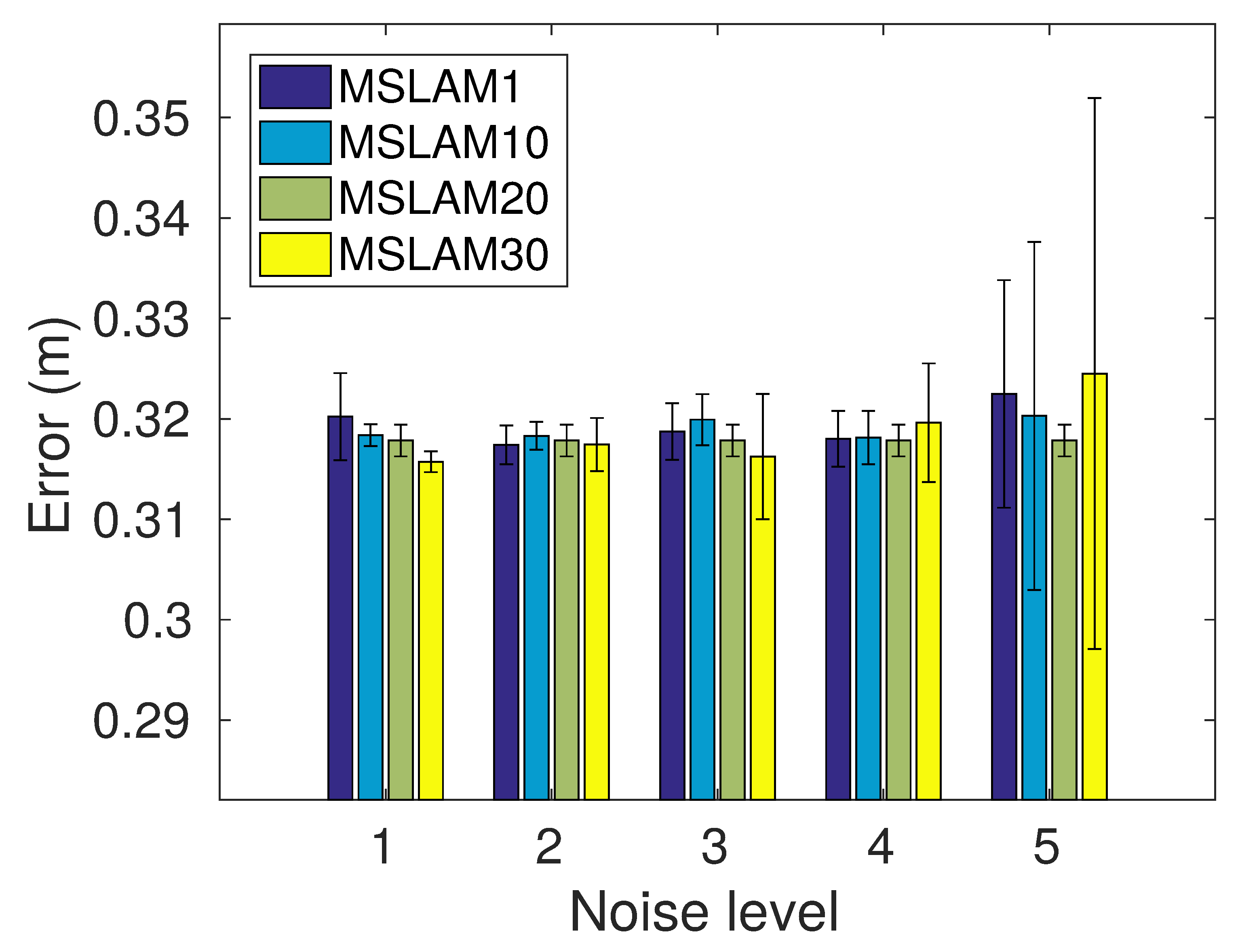
Figure 21 depicts the means and standard deviations of the MSLAM approach. The initial error barely influences the results except for error level 5, which leads to larger error variability. Nonetheless, even in the worst case, the standard deviation is only 0.021 m. It can also be observed that the delay to join the maps has almost no influence on the final results.
Figure 22a,b depicts the odometry corresponding to both trajectories corrupted with noise level 5. As can be observed, there is no visual resemblance between them and their non-corrupted counterparts in
Figure 12a,b.
Figure 22c,d shows the output of our proposed single-session SLAM using the corrupted trajectories, evidencing a huge improvement. Finally,
Figure 22e shows the output of MSLAM30. As can be observed, the results (therefore, the measured errors) are extremely similar to the case in which non-corrupted odometry was used (
Figure 12h).
Some additional experiments performed with larger noise levels show that the system leads to similar results except for noise levels that are not possible in real operation, such as errors in x or y that surpass the camera field of view. This is due to two main reasons. On the one hand, Algorithm 1 is particularly robust. Because of that, increasing the search radius of Equation (4) to account for larger odometric errors leads to larger execution times but not to an increase of false positives. Thus, large values for can be used even in low noise situations. On the other hand, global loop detection does not depend on the quality of the odometry. Accordingly, both map joining and the use of global loops to correct the joined trajectory are not affected by the noise level.
11. Conclusions
In this paper, we have presented a trajectory-based multi-session monocular SLAM approach aimed at underwater environments which has three main blocks: a visual odometer, two different loop detectors, and an optimizer. The visual odometer gives a first estimate of the camera motion in each single session. The single and multi-session loop closing detection add additional pose constraints to each individual sequence and between both sessions. Finally, the optimizer is in charge of improving the trajectories (intra-map optimization) and joining different sessions (map joining).
The main contributions of this paper are as follows: (a) Due to the lack of geometric information relating two different sessions, the multi-session loops are found using an image global signature (hash) fast matching based on HALOC which is already tested on underwater imagery. (b) The capacity of the map-joining algorithm to preserve the trajectory structure by adding a single link between the joined sessions; (c) to perform a delayed global graph optimization, reducing computational effort without loss of localization accuracy; and (d) to disaggregate sessions, reducing the computational cost whenever is necessary and joining them again later are improved. (e) A complete set of source codes that implement the whole process is available for the community.
Experimental results have been obtained from several video sequences taken with a single camera at subsea environments located in Mallorca. The results of the assessment of each particular component (odometry, loop detection, and optimization) in terms of quality and robustness evidence a high quality in the resulting trajectories. Moreover, the results using extremely corrupted odometry suggest that our proposal is barely influenced by odometric errors. On the other hand, the system has a couple of limitations, which are being addressed in the current ongoing work, and are out of the scope of this paper: (a) The approach is 2-D, and additional data concerning the constant altitude at which the underwater robot is moving is needed but easily obtainable by means of other sensors, such as a stereo altimeter or the DVL; this current approach is being evolved towards a 3-D one, taking into account the 6 Degrees of Freedom (DoF) of the vehicle, starting with the application of a 3-D odometer such as the well-known Viso2 Library [
53]. (b) The sooner the map joining task is performed, the best to increase the accuracy of the localization data; once both sessions are joined, the vehicle localization gets into a pure single session SLAM procedure, in which finding local loop closings is easier and they appear with more frequency than intersessions; and delaying the map joining delays inevitably the fine correction of the map.
The forthcoming work includes (a) implementing the whole system in C++, (b) setting out a strategy to get a trajectory ground truth of the underwater missions to be used in comparisons of our method with any other anchor-node-based methods, and (c) adapting the proposal presented in this paper to perform multi-robot visual SLAM.


