Cross-Shore Suspended Sediment Transport in Relation to Topographic Changes in the Intertidal Zone of a Macro-Tidal Beach (Mariakerke, Belgium)

Abstract

Sediment transport is a key element in intertidal beach morphodynamics, but measurements of sediment transport are often unreliable. The aim of this study is to quantify and investigate cross-shore sediment transport and the resulting topographic changes for a tide-dominated, sandy beach. Two fortnight-long field experiments were carried out during which hydrodynamics and sediment dynamics were measured with optical and acoustic sensors, while the beach topography was surveyed with a permanent terrestrial laser scanner. Suspended sediment was generally well-mixed and currents were largest at approximately 1.5 m above the bed, which resulted in a peak in sediment transport at 1/3 of the high tide level. The mean transport direction was onshore during calm conditions (wave height <0.6 m) thanks to tidal currents and offshore during energetic conditions due to undertow. Oscillatory transport was always onshore because of wave asymmetry but it was subordinate to mean transport. The intertidal zone showed an alternation of erosion and accretion with formation of morphological features during energetic (no storm) conditionsand smoothening of the morphology during calm conditions. A good qualitative and quantitative agreement was found between the daily cross-shore suspended load and beach volume changes, especially during calm conditions.

1. Introduction

The intertidal zone is highly dynamic, as it is subject to waves, tidal currents, and wind. Its dynamics have frequently been examined by relating hydrodynamic forcing directly to morphological response [1,2,3]. Sediment transport processes have been investigated to a lesser extent due to the complex motions and scales involved: from seconds to tidal cycles and beyond. Thus, most studies ofsediment transport have been qualitative [4,5,6] and only few have been successful in quantifying sediment transport in the intertidal zone [7]. Accurate measurements of sediment transport are crucial in order to improve our understanding and modelling capacities of the intertidal morphodynamics [8].

The high impact of breaking waves, rapidly changing bed levels, and variations in water level make it challenging to measure sediment transport in the intertidal zone. However, the advance of sophisticated sensors, such as high frequency optical backscatter sensors (OBS) and acoustic backscatter sensors, now allow for the examination of sediment transport more accurately and at an appropriate scale [9]. At the same time, equipment has been developed to measure the beach topography with a high spatial resolution. This provides more accurate estimations of beach volume changes compared to cross-shore profile measurements [10]. Therefore, sediment transport measurements can be appropriately validated.

In general, it is acknowledged that cross-shore sediment transport processes on beaches are controlled by the balance between onshore transport due to wave skewness/asymmetry and offshore transport by undertow [8,11]. However, sediment transport has been investigated most extensively on micro- to meso-tidal beaches, where waves are the dominant forcing [5]. Only a few studies have been specifically dedicated to the measurement of sediment transport on macro-tidal beaches and the associated intertidal bars (i.e., ridges and runnels) [12]. As a result, the role of tidal currents in sediment transport remains unclear.

This study presents a comprehensive set of records of (cross-shore) sediment transport and topographic response for a sandy, macro-tidal beach along the Belgian coast. Surveys were collected over two fortnight periods under low and moderate wave energy conditions (maximum wave heights of 0.7 and 1.5 m). The aim is to highlight the role of cross-shore sediment transport processes in the dynamics of a tide-dominated beach. As it was previously found that bed load only comprised 20% of the total load along the Belgian coast [11], the focus of this study is on suspended sediment transport.

2. Materials and Methods

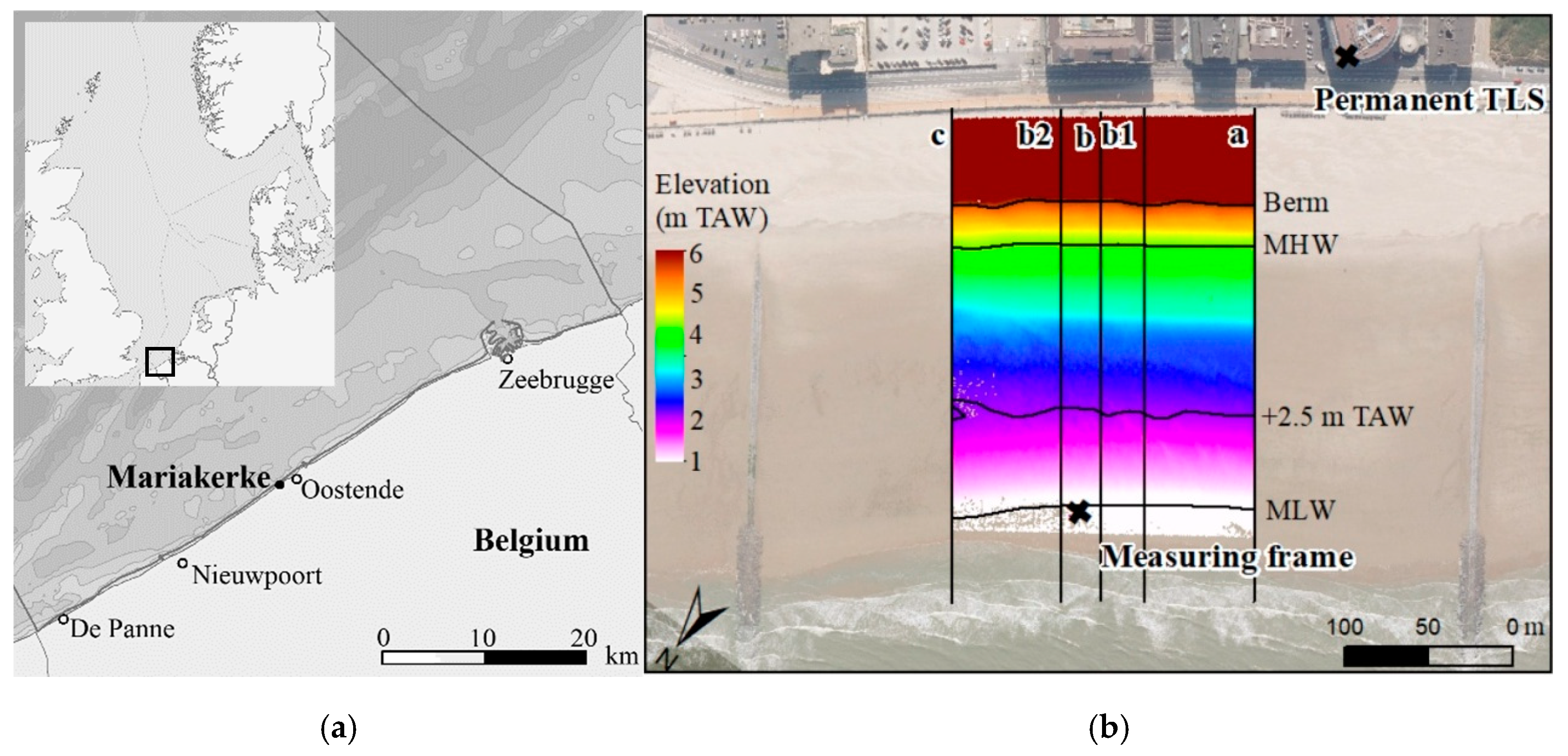
2.1. Study Site

This study was carried out at the beach of Mariakerke in Belgium (Figure 1). The Belgian coast is macro-tidal, with a tidal range of 3.5 m during neap and 5 m during spring tide [13]. This results in strong tidal currents (>1 m/s) in the nearshore area [13]. The tide is semi-diurnal and slightly flood dominant, with higher velocities during flood than during ebb. Wave energy is medium, with an average wave height of 0.5–1 m and an average wave period of 3.5–4.5 s. Offshore waves are mainly driven by westerly winds (WSW-NW). In combination with the SW-NE orientation (55–235°) of the Belgian coast, this results in a longshore drift towards the NE.

The beach at Mariakerke is characterized by a seawall and groins. Additionally, the beach is subject to regular small-scale beach nourishments and beach shaping. Large beach and underwater nourishments have been carried out since 2006 [14]. The intertidal beach is featureless, but the transition to the upper beach is characterized by a steep artificial berm of approximately 2 m high (37%). The intertidal beach is 160 m wide, and gently sloping (2%). It consists of well-sorted, medium sand with a median diameter of 325 µm. The natural trend of the beach at Mariakerke is erosive (−8 m³/m/yr), but thanks to replenishment it has been growing over the past decades (+4 m³/m/yr) [14].

2.2. Data Acquisition

Two fortnight-long measuring campaigns (7–20 November 2017 and 16–26 April 2018) were carried out to investigate marine forcing, sediment transport, and resulting topographic changes. Flow velocity, water level, wave conditions, and Suspended Sediment Concentrations (SSC) were measured with a frame at the mean low water (MLW) line (Figure 1b). The full beach topography was surveyed with a permanent TLS and the topography of five cross-shore profiles was measured with a real time kinematic-global navigation satellite system (RTK-GNSS; Figure 1b). Wind conditions were measured at the airport of Ostend, approximately 1 km from the study site.

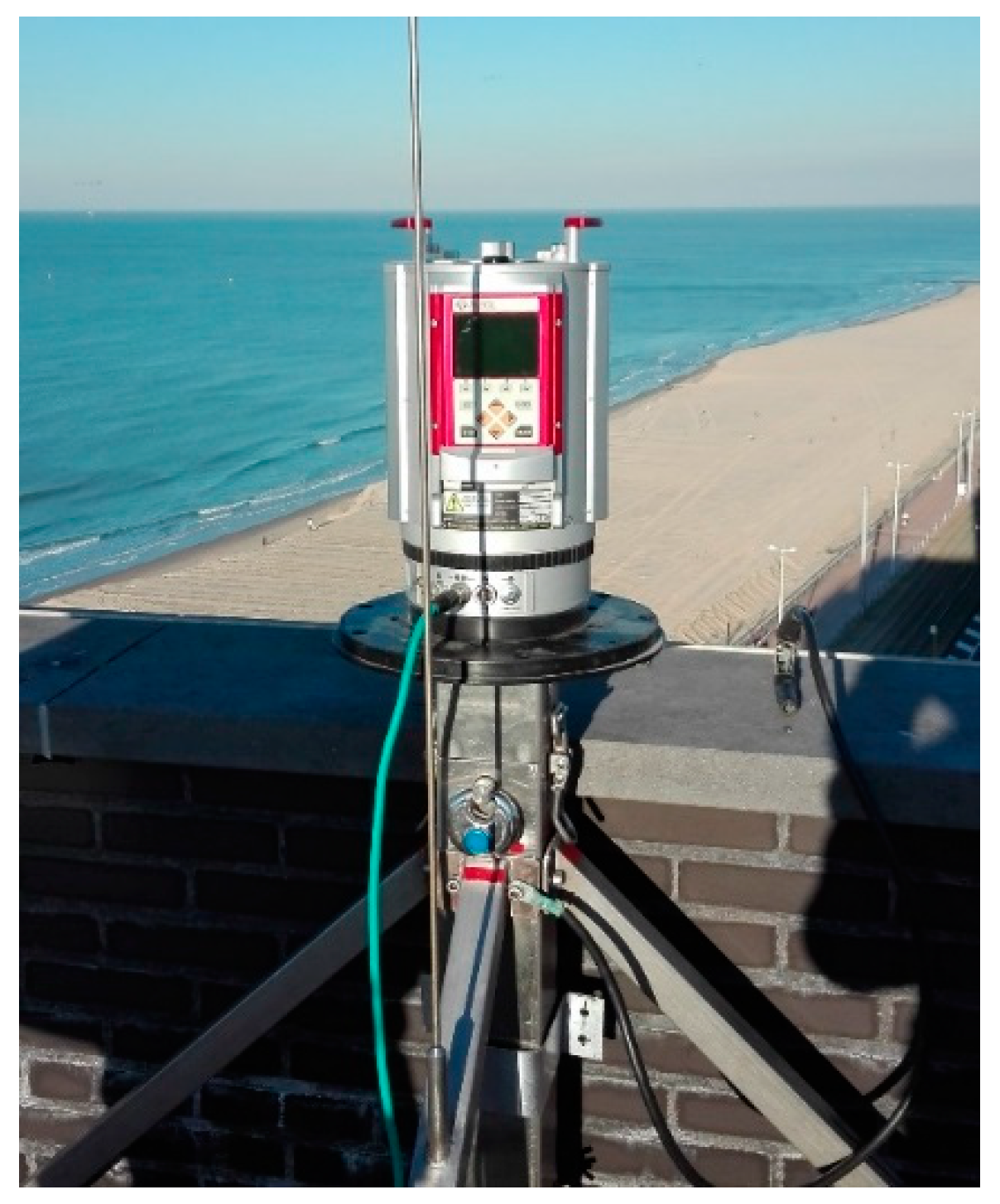
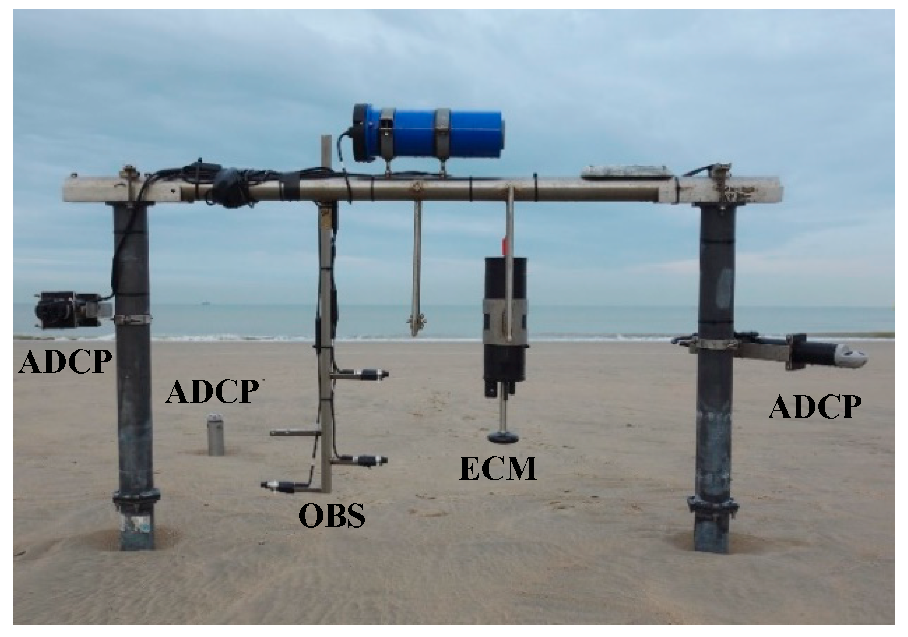
2.2.1. Hydrodynamics and Sediment Transport

The measuring frame (Figure 2) was equipped with three OBS (Campbell Scientific, Logan, Utah, USA) to measure turbidity, a proxy for SSC, at 10 cm (4 Hz), 30 cm (1 Hz), and 50 cm (1 Hz) above the bed. Furthermore, two Acoustic Doppler Current Profilers (ADCPs, Aquadopp model; Nortek Group, Rud, Norway) were mounted on the frame to measure profiles of flow velocity and acoustic backscatter, another proxy for SSC. Both were mounted at 70 cm above the bed and measured 9 cells of 5 cm, but one was looking up (1 Hz) and one was looking down (4 Hz). Additionally, an upward-looking ADCP was deployed in the sand which measured profiles with 14 cells of 30 cm (1 Hz, 5-minute bursts) to cover the part of the water column above 1.2 m. An Electromagnetic Current Meter (ECM; Valeport, Devon, UK) was mounted 50 cm above the bed. This sensor was set to measure flow velocity and pressure (8 Hz, 1 minute every 10 minutes) from which wave height and wave period were calculated.

The data was treated by removal of the data when the equipment was exposed to the air and the obvious outliers. Flow velocity was converted to cross- and alongshore flow velocity in order to determine the on- and offshore sediment transport rates. The cross-shore sediment flux was calculated by multiplying SSC and flow velocity. The mean and oscillatory component of the cross-shore suspended sediment transport were also calculated separately to investigate the contribution of mean currents versus the contribution of waves ($\overline{u·c}=\overline{u}·\overline{c}+\overline{u^{\prime }·c^{\prime }}$, where u is flow velocity and c is SSC). The total suspended load per tidal cycle was calculated by vertically integrating the sediment transport over the water column and by integrating the transport over the tidal cycle. It was converted to a volume using a sediment density of 2000 kg/m³ (typical density of wet sand).

Sediment transport was compared to the velocity skewness (U_sk) that was calculated from the cross-shore flow velocity (u_cross): $U_{sk}=\langle u_{cross}^3\rangle /\langle u_{cross}^2\rangle$ [15]. Positive and negative velocity skewness are indicative of onshore and offshore transport, respectively, as it is assumed that sediment transport is proportional to u³. Sediment transport was also compared to wave steepness, to investigate the effect of wave conditions on suspended sediment transport. Wave steepness was calculated as $Wavesteepness=H/L$, where H is wave height and L is wave length. Wave length was calculated depending on the water depth and wave height with the dispersion equation: $L=g{T}^2\tanh (2\pi h/L)/2\pi$ or the shallow water approximations: $L=T\sqrt{gh}$, where h is water level, g is the gravitational acceleration, and T is wave period [16]. In this study significant wave period (T_sig) and height (H_sig) were used.

Turbidity measured by the OBS was converted to SSC with a calibration based on in-situ samples (Appendix A). The acoustic backscatter from the ADCP (Amp) was corrected for acoustic spreading and water absorption [17]: $EI=0.43Amp+20\log (R)+2a_{w}R$, where R is the range along the acoustic beam and a_w is the water absorption (1.0637 dB/m here). EI, the range normalized echo intensity (dB), was converted to SSC based on the OBS measurements in the lowest part of the water column. The relationship between tidally-averaged SSC based on acoustic backscatter and optical backscatter (Figure 3) was significant with a p-value of 1.44∙10⁻⁵ (<0.05, R² of 0.45), although instantaneous differences were large.

2.2.2. Beach Topography

TLS, or light detection and ranging (LiDAR), has been used successfully to survey the beach topography [18,19,20]. TLS is a highly automated active remote sensing technique, composed of an Electromagnetic Distance Measuring (EDM) technique to derive a backscatter-based distance by measuring the circulation time of a pulse or the wavelength difference of a continuous wave. The coordinates of a point on the reflecting surface are determined by transmitting signals from a measuring instrument of which the orientation and the coordinates are known or fixed in three dimensions.

A time-of-flight-pulse-based Riegl^® VZ-2000 terrestrial LiDAR (Riegl, Horn, Austria) was installed on a 42 m high building near the study area (Figure 4) and data was acquired similar to [20]. The permanent TLS scanned the intertidal and dry beach on an hourly basis over a period of one year. The scanner was installed on a stable frame and protected by weather-proof housing. The scan data werecalibrated using a truth set of reference points to enhance the accuracy and precision. The point density of the permanent TLS data varies between more than 250 points/m² in the southwestern part of the dry beach and 1 point/m² in the northeastern part of the intertidal beach. It appears that the useful range of the scanner is limited to 200 m. The vertical accuracy (root mean square error) of the TLS data was found to be 1–3 cm.

The 3D point cloud data from the permanent TLS wereinterpolated to a rasterized (1 × 1 m) digital elevation model (DEM) using inverse distance weighting (IDW). DEMs of differences (DoDs) were generated by subtracting the DEMs of subsequent days. For each day, the volume of the intertidal zone was calculated. The intertidal zone was defined as the area between the MLW (+1.39 m TAW; Belgian reference level, i.e.,relative to the lowest astronomical tide) and the toe of the berm (+5.30 m TAW). It was decidedto extend the area above the mean high water (MHW, +4.39 m TAW) line because it was assumed that the narrow strip between the MHW line and the berm was dominated by hydrodynamic forcing.

Wet areas of the beach yield poor reflection of the laser scan signal, which sometimes resulted in a lack of data in the lowest part of the intertidal zone. Beach topography was therefore also measured with RTK-GNSS (Trimble, Sunnyvale, California, USA) during low tide in order to fill the gaps in the permanent TLS data. Five cross-shore profiles were surveyed: one central profile (b), two profiles at 25 m from the central profile (b1 and b2), and two distant profiles 75 m from the central profile and 75 m away from the groins (a and c; Figure 1). The RTK-GNSS profiles were measured at an interval of 1 m in the cross-shore direction with a vertical accuracy of 2–4 cm [21]. The volume of the intertidal beach was calculated from the topographic profiles. Volumes were calculated for each profile separately using trapezoidal rules. The volumes of all profiles (a, b1, b, b2, and c) were averaged and daily volume changes were calculated.

3. Results

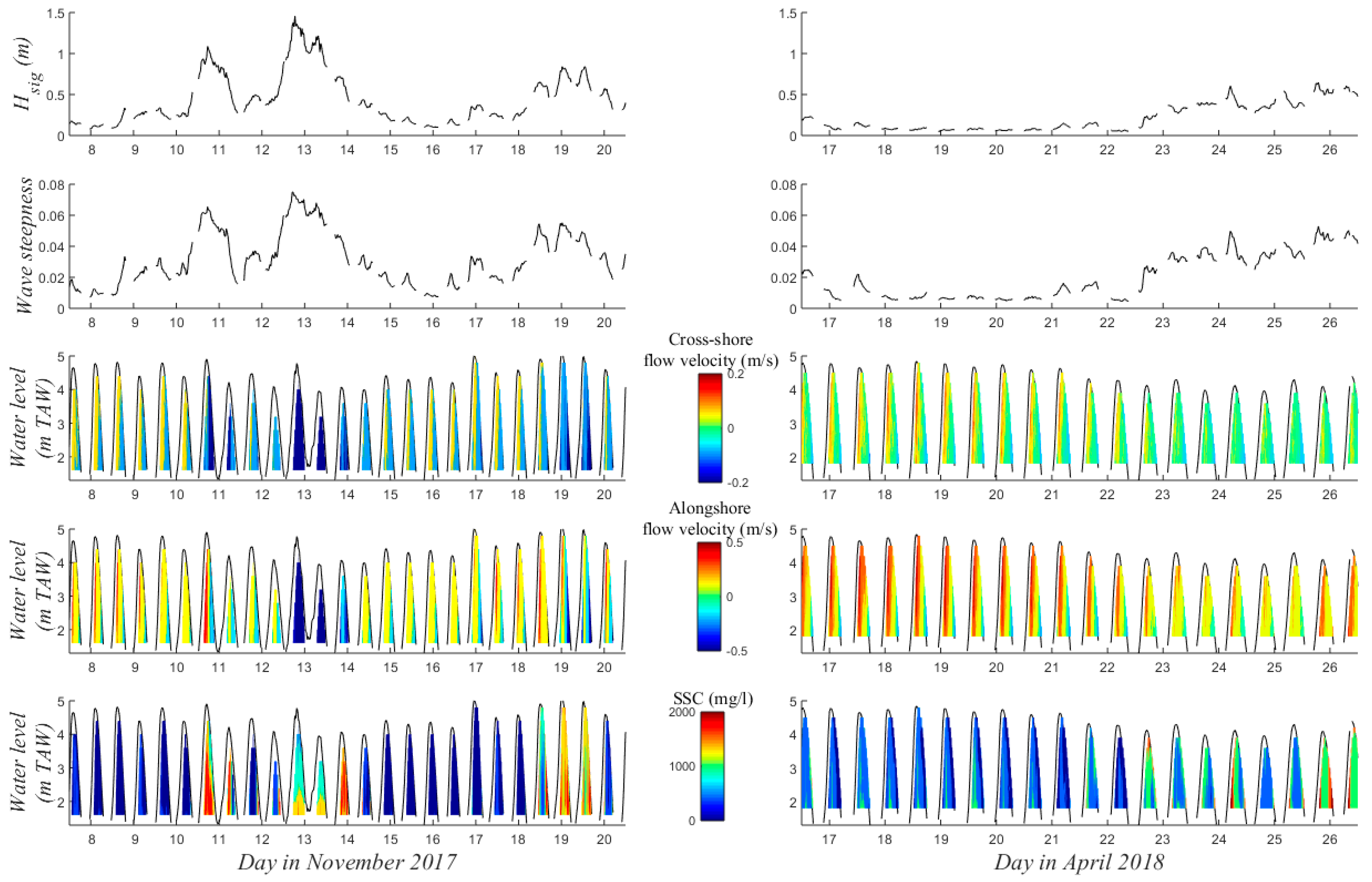
3.1. Hydrodynamics

The hydrodynamic conditions and suspended sediment concentrations during the two periods of data collection (November 2017 and April 2018) are summarized in Figure 5. The wave conditions were energetic in November with peaks in wave height of 1.46 m in the intertidal zone, corresponding to an offshore measured wave height of 3.15 m, while peaks in wave steepness reached 0.075. The average wave height over the two weeks was 0.42 m. In April the waves were calm with an average and maximum wave height of 0.21 m and 0.65 m respectively. The water level exceeded the storm threshold of 5 m TAW that was defined for the Belgian coast [13] on 16 November when the water level reached 5.01 m TAW. This threshold was approached on 10 and 19 November, when the water level reached 4.91 and 4.98 m TAW, respectively. Currents were directed onshore with a large alongshore component during flood, while ebb currents were directed offshore. Flow velocity was highest at approximately 1.5 m above the bed (2.9 m TAW), which corresponds to 1/3 of the high water level. Strong offshore and southwesterly directed currents were observed when waves were energetic (>0.6 m). The average SSC was 1056 mg/L in November and 839 mg/L in April. SSC was especially high when energetic waves occurred, such as between 10 and 14 November. SSC was on average 500–1000 mg/L higher during the flood phase than during the ebb phase. Generally, the suspended sediment was well-mixed over the water column, but SSC were highest near the bed when waves were energetic.

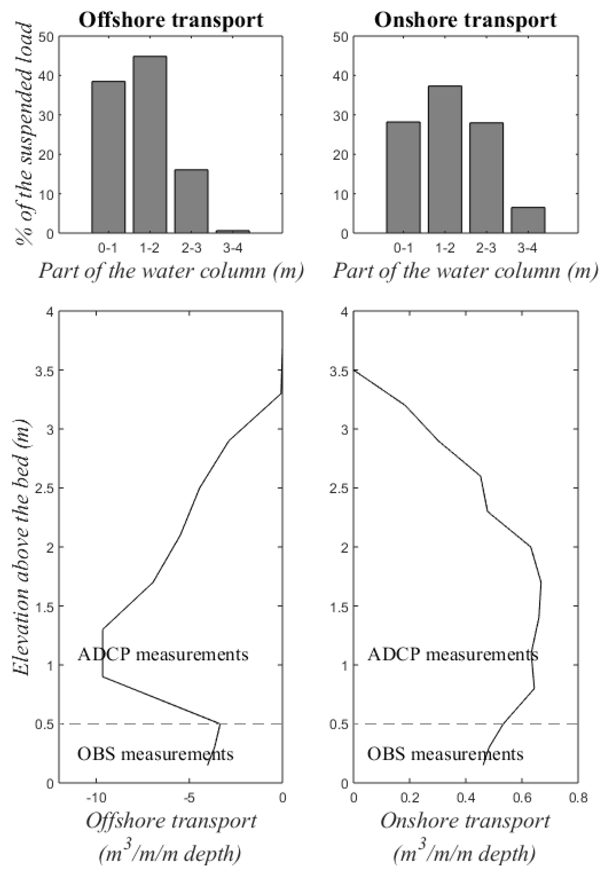
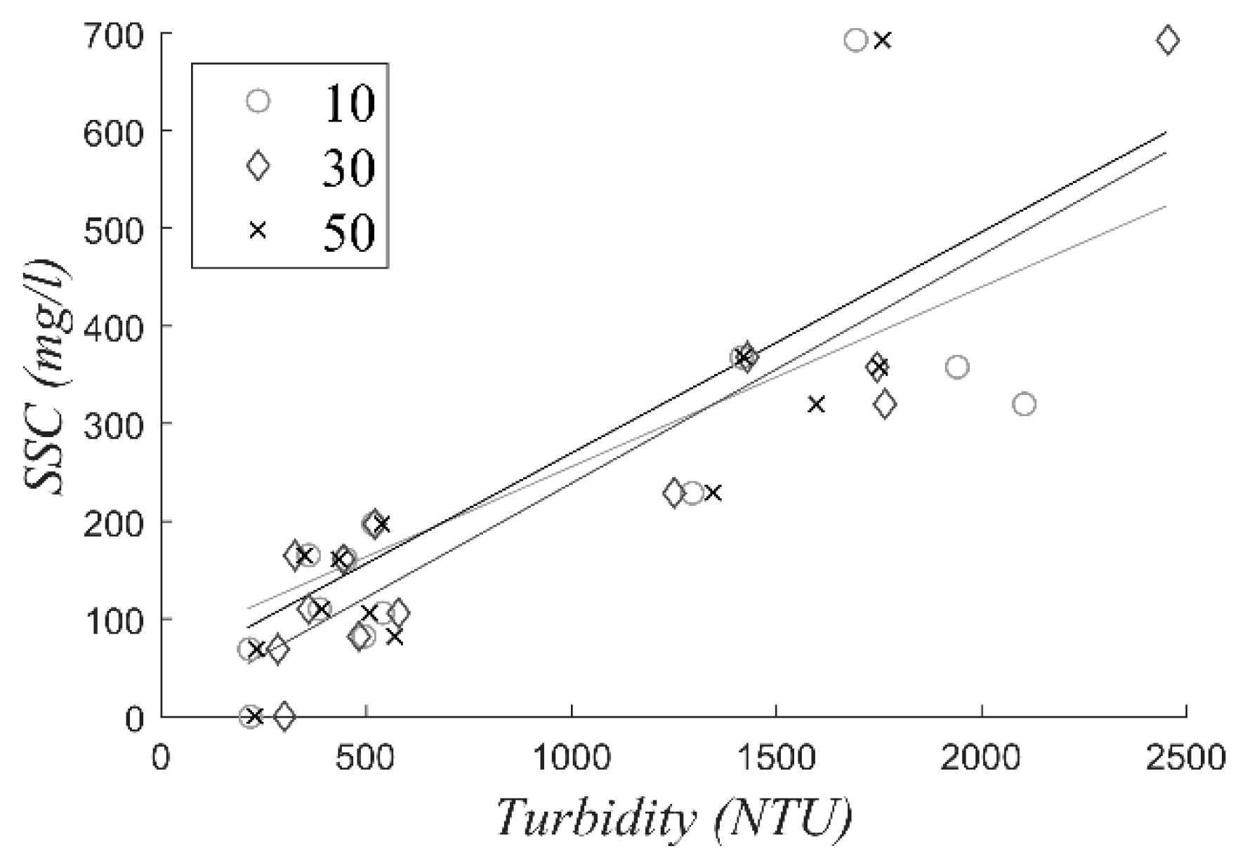
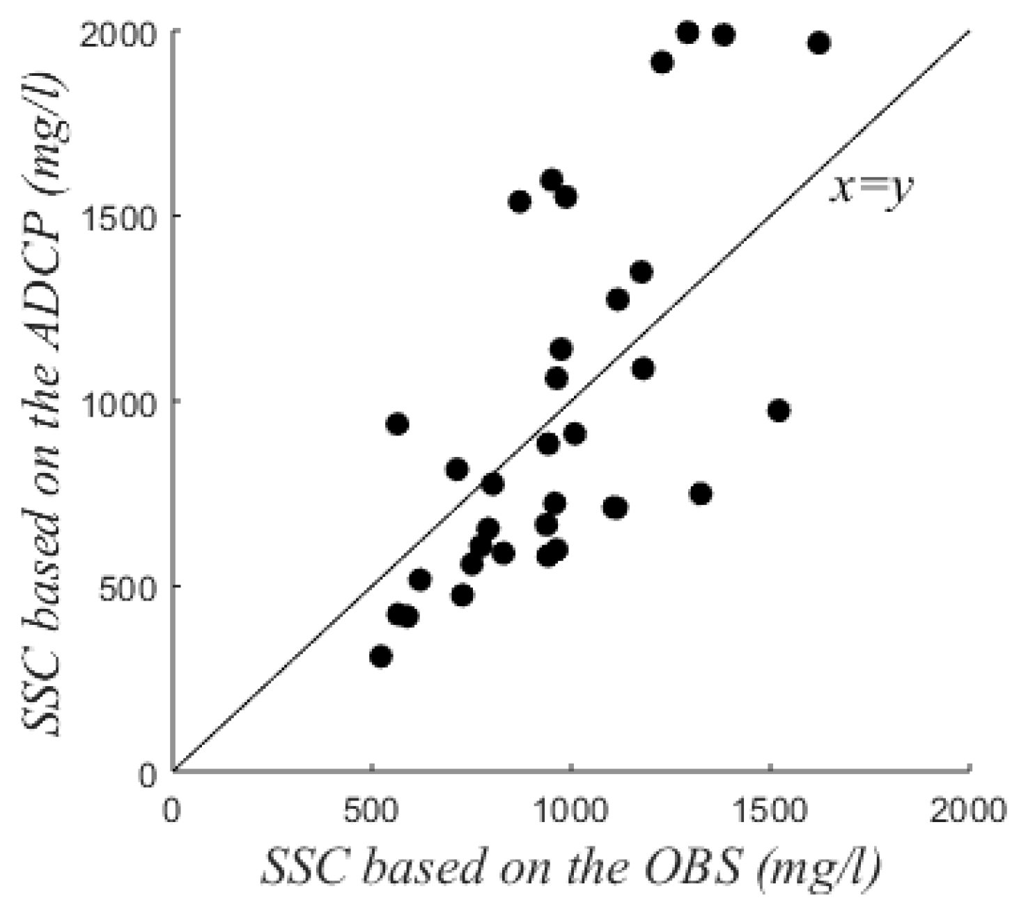
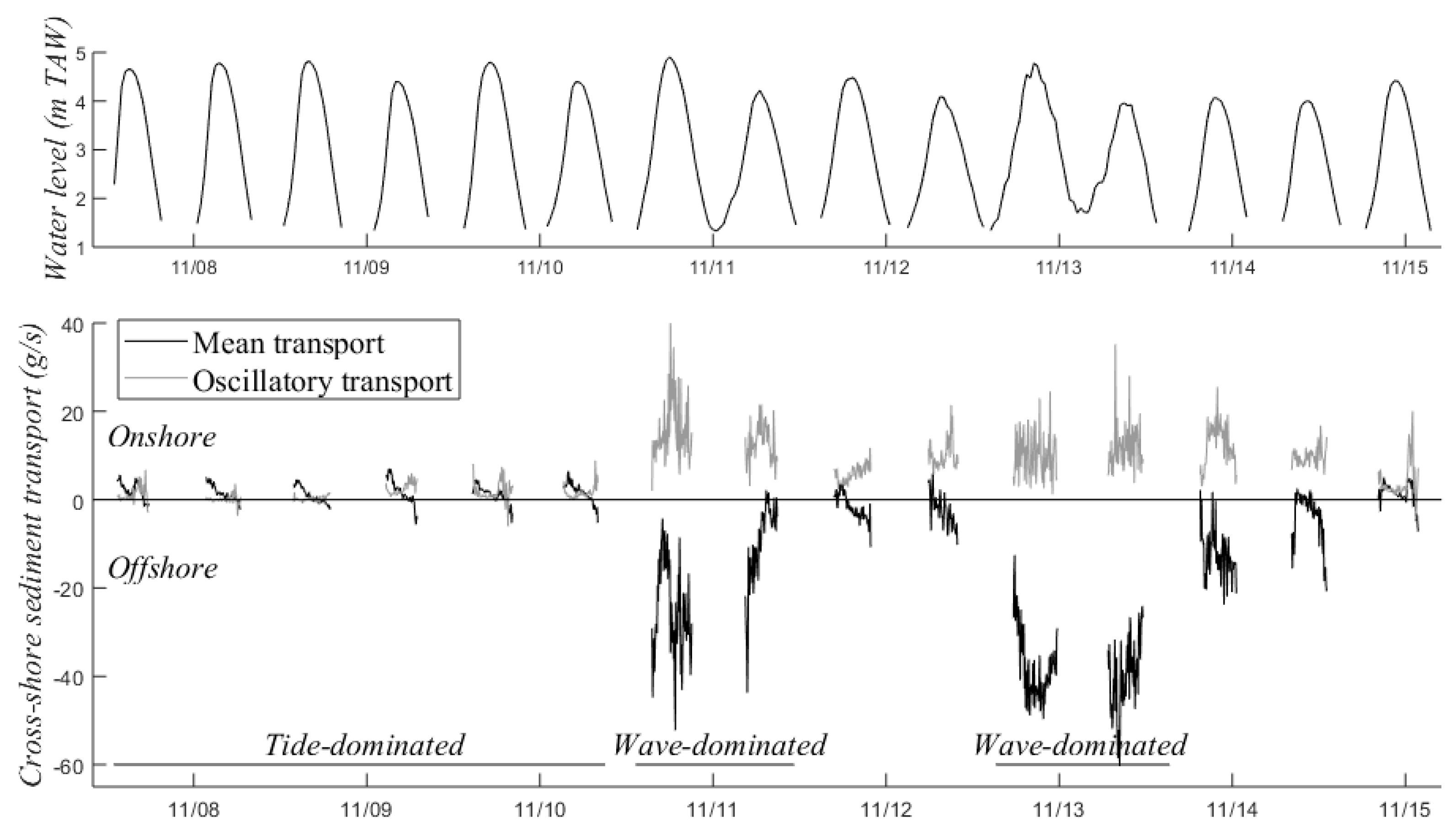
3.2. Suspended Sediment Transport

Mean and oscillatory cross-shore suspended sediment transport are presented in Figure 6 for the first week of the November 2017 campaign, which showed the widest variety of hydrodynamic conditions. The first days (7–10 November) were tide-dominated, with calm waves and spring tide conditions. Mean transport dominated and was onshore during the flood and offshore during the ebb phase. Oscillatory transport was onshore because of wave asymmetry (larger onshore velocities than offshore velocities) and was especially large around low tide due to waves breaking near the measuring frame. On 10/11 and 12/13 November the conditions were wave-dominated, with wave heights exceeding 0.6 m. Mean transport still dominated, but was mainly offshore because of strong undertow, the return flow of the waves. Oscillatory transport was still directed onshore but was stronger than under tide-dominated conditions. It was relatively constant indicating that waves were constantly breaking at the MLW line. Figure 6 illustrates the sediment transport at 10 cm above the bed, but these findings apply to the entire water column.

The cross-shore suspended load per tidal cycle was compared to the velocity skewness and wave steepness (Figure 7). The velocity skewness was positive when waves were small because of the shape of the incident waves. The velocity skewness became negative when waves became larger (wave steepness >0.025) due to the strong undertow. Net transport was offshore when the velocity skewness was negative, whereas transport was onshore when the velocity skewness was positive. Consequently, sediment transport was onshore when wave steepness was small and offshore when wave steepness was large.

To investigate the sediment transport over the water column, cross-shore suspended sediment transport was tidally-integrated. This was done for slices of 1 m (Figure 8, top) and slices of 30 cm (the maximum cell size of the ADCPs; Figure 8, bottom) of the water column. The distribution of the total suspended load over the water column per slice of 1 m is shown for offshore and onshore transport events. Suspended sediment transport was the largest between 1 and 2 m above the bed. Sediment transport was more homogenous during calm conditions and more concentrated near the bottom during energetic conditions. The maximum offshore transport was significantly larger than the maximum onshore transport (9.7 vs. 0.7 m³/m/m depth). The suspended sediment transport peaked at 1 m above the bed during offshore transport events. During such events the SSC was largest near the bed, while offshore flow velocities were highest at 1–1.5 m above the bed. During onshore transport events the suspended sediment load was well-mixed over the water column. A small peak in transport was observed at 1.5 m above the bed. The total suspended load decreased towards the top of the water column (>2 m), because it represents a smaller period of time.

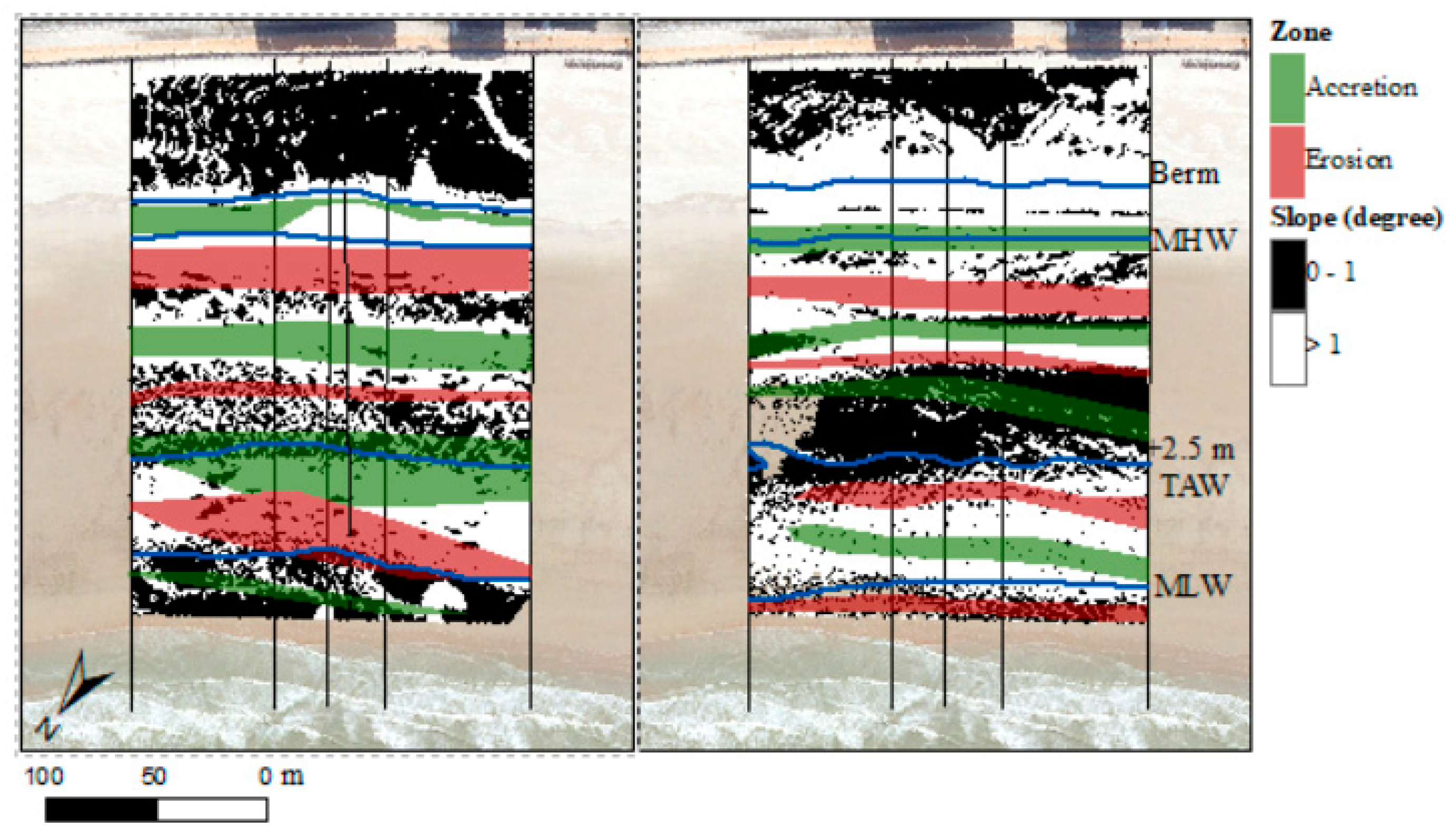
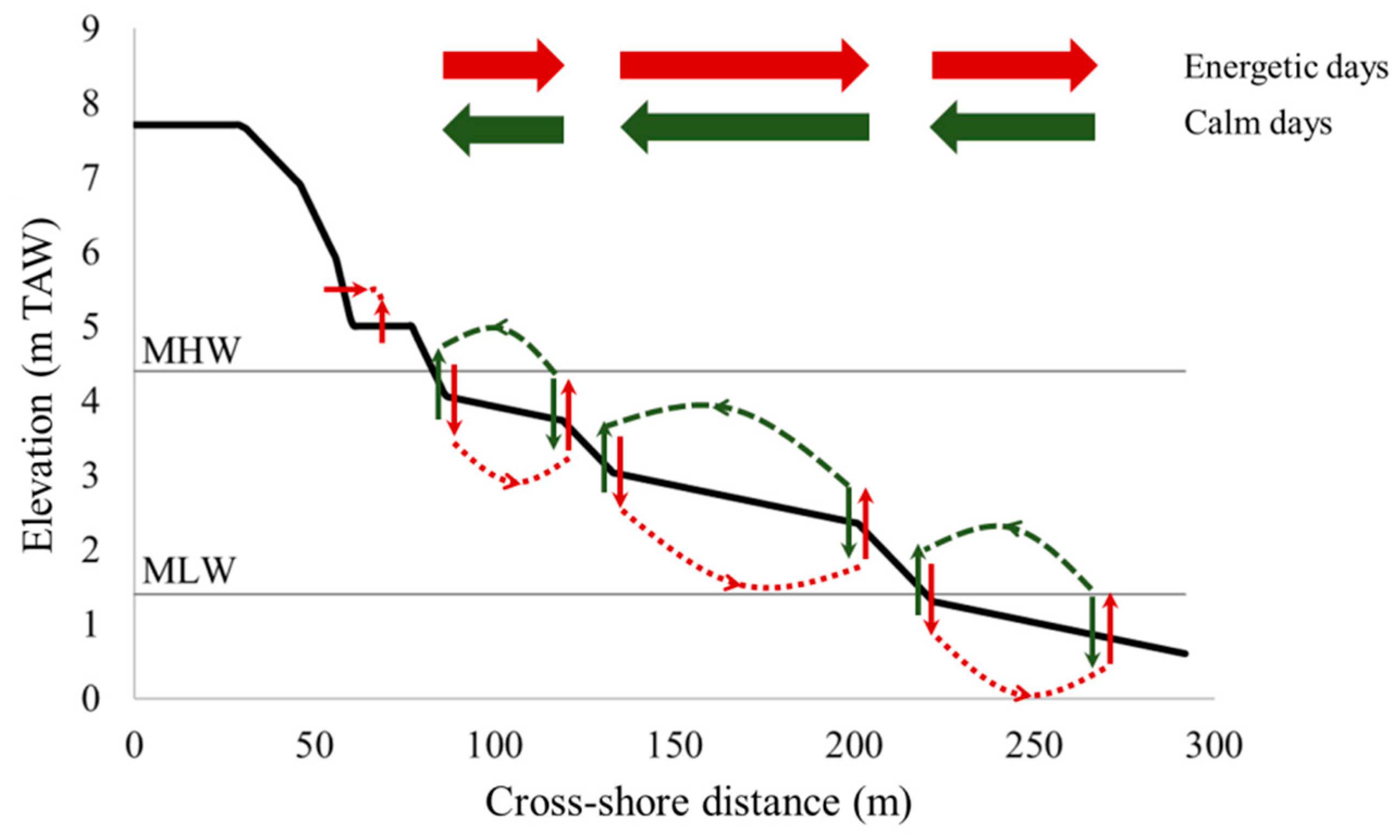
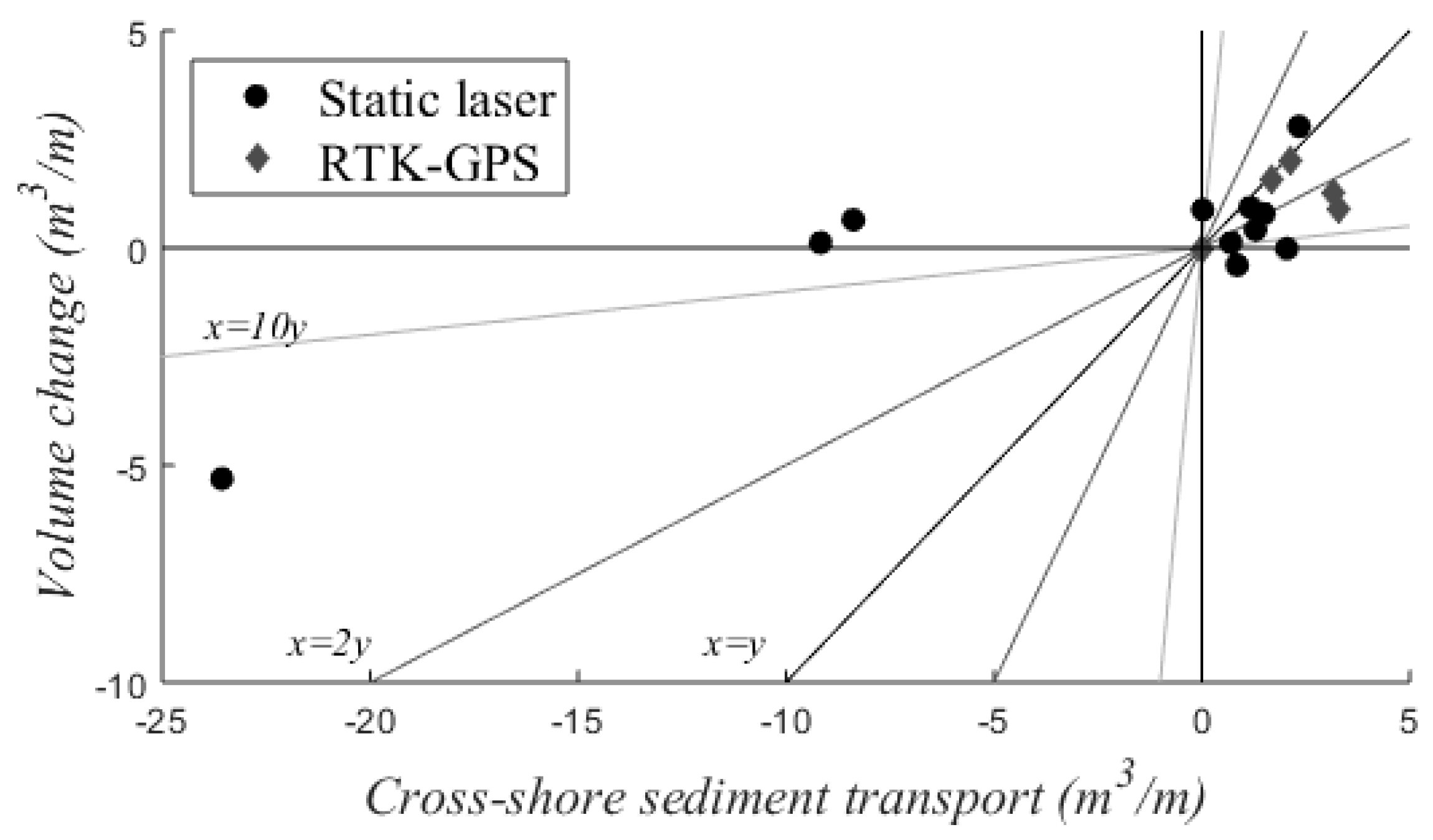
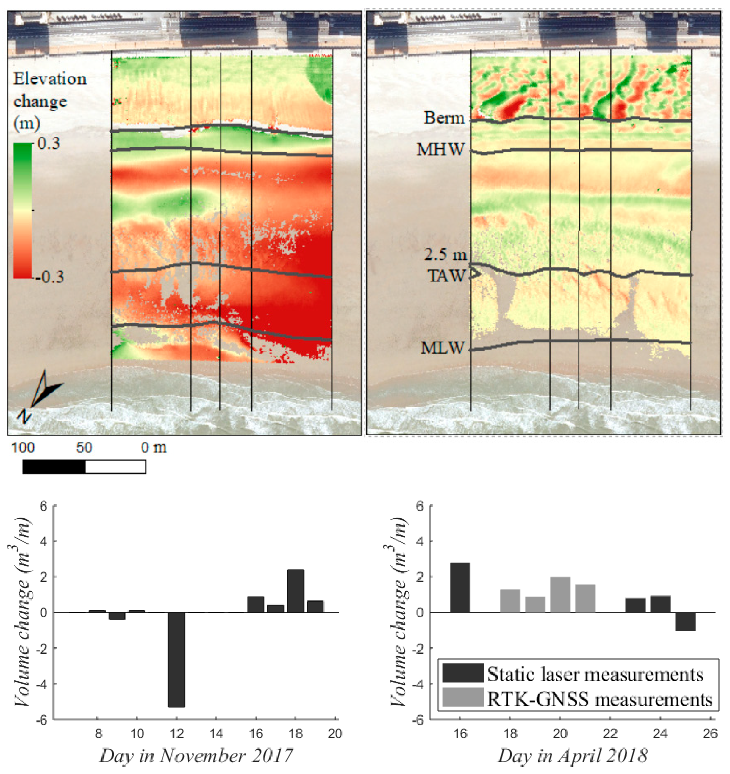
3.3. Topographic Change

Figure 9 represents the net topographic change over the two fortnight measuring campaigns (red = erosion, green = accretion) and the daily volume changes of the intertidal zone. Bed level changes in the intertidal zone were in the order of centimeters to decimeters over the fortnight periods. Wind-driven topographic changes of several decimeters were also observed on the upper beach above the berm. In November the intertidal beach predominantly eroded, with a loss of sediment of 18.6 m³/m over the campaign. Strongest erosion was observed on 12 November, while most other days the beach was stable or even grew. In April the intertidal beach gradually built-up, gaining 5.1 m³/m over the campaign.

An alternating pattern of erosion and accretion was detected from daily DoDs when the suspended load was large. Figure 10 shows the zones of maximum accretion and erosion for the three days with most offshore sediment transport (10, 12, and 19 November; left) and the three days with most onshore transport (17, 18, and 19 April; right). The erosion and accretion patterns were compared to the beach slope, which was subdivided into sloping (>1°) and relatively flat (<1°). Erosion was observed at the bottom of the slopes during offshore transport events, while accretion was observed at the top of these slopes. During onshore transport events accretion was observed at the bottom of slopes and erosion at the top. A part of the sediment that was eroded from the intertidal zone during energetic conditions was deposited just below the MLW line. This sediment was returned to the beach during calm conditions.

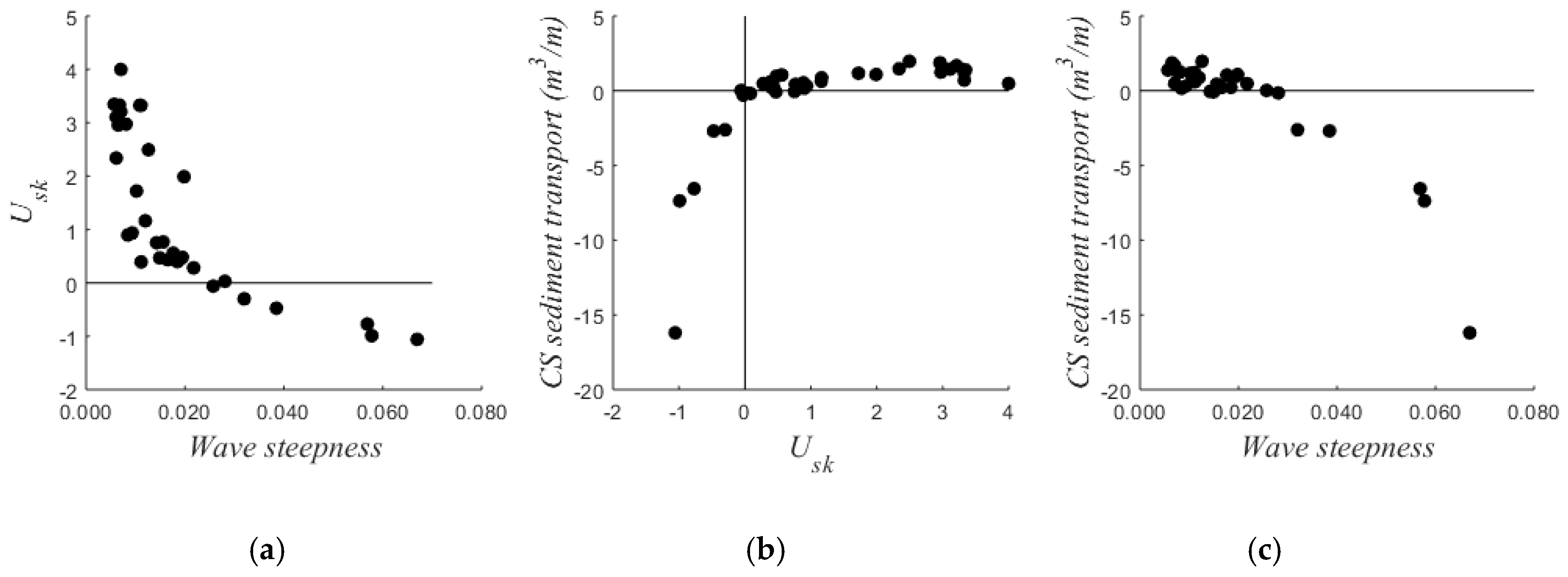
4. Discussion

Sediment was transported to the beach by tidal currents and by wave-induced oscillatory transport under calm conditions (wave steepness <0.025). Sediment was transported offshore by strong undertow during energetic conditions. The dominance of mean transport over oscillatory transport is in agreement with previous observations on the Belgian and other macro-tidal coasts [11,22]. However, the mean cross-shore transport by tidal currents may have been enhanced by the groins, which divert the tidal currents to more cross-shore. The suspended sediment was well-mixed over the water column, resulting in a peak of sediment transport at 1.5 m above the bed. Other studies usually observe highest suspended sediment transport rates close to the bed [7,12,23]. However, most studies ofsuspended sediment transport have been performed on wave-dominated beaches, while on macro-tidal beaches tidal currents play an important role in keeping sediment in suspension and transporting sediment.

Schematized sediment transport and topographic response across the intertidal zone is shown in Figure 11. It appears that morphological features are developed during energetic conditions around 80 m, 120 m and 210 m cross-shore distance. The beach morphology is smoothened during calm conditions. It was previously found that intertidal bars (i.e., ridges and runnels) are formed along the Belgian coast by standing long waves [24]. This type of bar system is exclusive to dissipative, macro-tidal beaches with sufficient sediment supply and a fetch-limited wave climate, which are common along the North Sea coast [12,24,25]. Here, long waves (period >10 s) were over 40 cm during energetic conditions, while they were 5 cm on average during calm conditions. Most likely, the coupling between short and long waves lead to positions of sediment convergence and divergence [26], which resulted in bar formation. However, they never fully develop due to the presence of the groins [27].

The total cross-shore suspended sediment load is compared to intertidal beach volume changes in Figure 12. Topographic changes suggest the same transport direction as the underwater measurements for 81% of the time. Generally, they are also in the same order of magnitude (75%) or even less than two times over- or underestimated (38%) by the suspended sediment load. The suspended sediment load was on average 1.4 times larger than the observed topographic change for calm conditions (onshore sediment transport). Energetic conditions were less frequent than calm conditions, but based on the limited observations it can be concluded that the total suspended load does not predict beach changes very well. The erosion of the intertidal zone occurred only during one out of the three days with offshore transport, whereas the beach was stable during the other two days. Reasons for differences between the measured sediment transport and observed volume changes include exchange of sediment with the dry beach, gradients in alongshore sediment transport, bed load transport, sediment transport by swash action and measurement inaccuracies.

It was assumed that all sediment entering or leaving the intertidal zone passed the low water line. However, undermining of the berm was observed when waves were high (Figure 13). This resulted in an input of sediment from the upper beach to the intertidal zone. This was reaffirmed by the presence of sand accumulation near the toe of the berm (around 5.1 m TAW) during energetic conditions (Figure 10). Under these conditions the water level reached 4.8–5.0 m TAW and waves reached the toe of the berm. Figure 14 shows hourly observations of the toe of the berm on 12 November when the maximum water level reached 4.8 m TAW. The elevation of the toe of the berm increased with 14 cm during high tide. This corresponded to a deposited volume of 0.88 m³/m, which explains 17% of the change in the intertidal zone.

Sediment exchange between the intertidal zone and the upper beach may also result from wind activity. Wind-driven transport in the intertidal zone has been investigated on various occasions [28,29], but rarely as a part of the sediment budget. Some studies attributed significant intertidal beach erosion/accretion to transport by wind [30], but aeolian transport remains uncertain in the sediment budget when relating topographic changes to underwater transport. Here, aeolian sand transport was quantified based on the hourly observations of the toe of the berm on 12 November (Figure 14). This was the most energetic day with wind speeds up to 22 m/s blowing onshore, which were optimal conditions for sand transport in the intertidal zone as observed in the field. Sediment transported by the wind was deposited in front of the berm, resulting in a rise of the berm toe of 4 cm while the intertidal zone was not affected by hydrodynamic processes (Figure 14, second low tide). This corresponds to a deposited volume of 0.25 m³/m (5% of the total change). Sediment transport from the intertidal zone to the upper beach was even smaller, as the majority of the wind-blown sediment was intercepted by the berm.

Sediment exchange between the intertidal zone and the upper beach by aeolian transport and by waves undermining the berm was thus limited. Sediment exchange between the study site and adjacent beaches was most likely significant though, but could not be investigated with the current measuring set-up. It was demonstrated that gradients in alongshore sediment transport can result in significant topographic changes along the Belgian coast [31], similar to other sandy beaches [5,7]. Gradients in alongshore sediment transport will thus explain some of the differences between the measured sediment load and observed topographic changes.

Differences between the total suspended load and beach volume changes may also be explained by the sediment transport that was not covered by the measurements: bed load transport and transport under low water levels. It was presumed that the contribution of bed load transport was small based on [11] who argued that only 20% of the total load near the study site consisted of bed load transport. Sediment transport measurements were limited to a water depth of 40 cm (64% of the time). Part of the sediment transport under breaking waves (8% of the time) and the transport by swash (5% of the time) were not covered. The remainder of the time, the intertidal zone was not affected by hydrodynamic processes (23%). Previously, it was found that significant sediment transport can occur under low water levels [31,32,33,34,35]. Therefore, disagreements between the suspended load and observed topographic changes may thus be explained by hydrodynamic processes for the 13% of the time that was not covered by the measurements.

Despite these inaccuracies, a good relationship between sediment transport and topographic change was established under calm conditions. This proves the added value of acoustic backscatter to survey sediment transport over the entire water column and the use of a permanent TLS to survey the beach topography with a high accuracy.

5. Conclusions

In order to improve our understanding and modelling capacities of the intertidal zone, a major focus of coastal research is to include sediment transport in studies about intertidal beach morphodynamics. This study investigated cross-shore sediment transport and resulting topographic changes for a tide-dominated, sandy beach on a daily scale. This was done based on insitu measurement of the hydrodynamics, suspended sediment concentrations, and beach topography.

The suspended sediment was generally well-mixed, but during energetic conditions the SSC was the highest near the bed. Flow velocity was highest at approximately 1.5 m above the bed. As a result, the suspended sediment transport was well-mixed over the water column with a peak in transport at approximately 1/3 of the (maximum) water column. This peak was most pronounced during energetic conditions due to strong flow velocities and higher SSC close to the bottom.

Sediment transport by mean currents was dominant over oscillatory sediment transport. Mean sediment transport was onshore during calm conditions because of tidal currents and offshore during energetic conditions because of undertow. Oscillatory transport was always onshore because of the flood dominance of the waves. The combination of mean and oscillatory currents resulted in a positive velocity skewness and onshore sediment transport when waves were small (wave height <0.6 m or wave steepness <0.025). The velocity skewness was negative and sediment transport was offshore when waves were large.

Changes in beach topography showed an alternating pattern of erosion and accretion. Morphological features were formed during energetic conditions (for an offshore wave height up to at least 3.15 m) and smoothened during calm conditions. At least a part of the sediment that was eroded from the intertidal zone during energetic conditions was deposited just below the low water line. During calm conditions, this sediment was transported back to the intertidal zone.

A good relationship between measured sediment transport and intertidal beach volume changes was obtained by using acoustic backscatter to survey sediment transport over the full water column and a permanent TLS to accurately measure beach topography. The suspended load and daily intertidal beach volume changes were in the same direction and order of magnitude for 75% of the investigated days. Especially during calm days with onshore transport, the relationship between the suspended load and intertidal beach volume changes was good, although the transport measurements overestimated the volume change (1.4 times). Energetic conditions were less well represented, but it seemed that the measured sediment transport greatly overestimated the volume changes observed in the intertidal zone. This was attributed to input of sediment from the dry beach, gradients in alongshore sediment transport, bed load transport, and transport by swash. The contribution of aeolian transport was found to be negligible (maximum 0.25 m³/m/day, corresponding to 5% of the total change) even though wind conditions were energetic (up to 22.6 m/s). Nevertheless, a good relationship between measured sediment transport and observed topographic changes was obtained to allowthe improvement of our understanding and to support the modelling capacities forthe intertidal zone.

References

- Anthony, E.J.; Levoy, F.; Monfort, O. Morphodynamics of intertidal bars on a megatidal beach, Merlimont, Northern France. Mar. Geol. 2004, 208, 73–100. [Google Scholar] [CrossRef]
- Reichmüth, B.; Anthony, E.J. Tidal influence on the intertidal bar morphology of two contrasting macrotidal beaches. Geomorphology 2007, 90, 101–114. [Google Scholar] [CrossRef]
- Austin, M.; Scott, T.; Brown, J.; MacMahan, J.; Masselink, G.; Russell, P. Temporal observations of rip current circulation on a macro-tidal beach. Cont. Shelf Res. 2010, 30, 1149–1165. [Google Scholar] [CrossRef]
- Aagaard, T.; Kroon, A.; Andersen, S.; MøllerSørensen, R.; Quartel, S.; Vinther, N. Intertidal beach change during storm conditions; Egmont, The Netherlands. Mar. Geol. 2005, 218, 65–80. [Google Scholar] [CrossRef]
- Sedrati, M.; Anthony, E.J. Storm-generated morphological change and longshore sand transport in the intertidal zone of a multi-barred macrotidal beach. Mar. Geol. 2007, 244, 209–229. [Google Scholar] [CrossRef]
- Turner, I.L.; Russell, P.E.; Butt, T. Measurements of wave-by-wave bed-levels in the swash zone. Coast. Eng. 2008, 55, 1237–1242. [Google Scholar] [CrossRef]
- Tonk, A.; Masselink, G. Evaluation of Longshore Transport Equations with OBS Sensors, Streamer Traps and Fluorescent Tracer. J. Coast. Res. 2005, 21, 915–931. [Google Scholar] [CrossRef]
- Masselink, G.; Austin, M.; Tinker, J.; O’Hare, T.; Russell, P. Cross-shore sediment transport and morphological response on a macrotidal beach with intertidal bar morphology, Truc Vert, France. Mar. Geol. 2008, 251, 141–155. [Google Scholar] [CrossRef]
- Aagaard, T.; Hughes, M.; Baldock, T.; Greenwood, B.; Kroon, A.; Power, H. Sediment transport processes and morphodynamics on a reflective beach under storm and non-storm conditions. Mar. Geol. 2012, 326–328, 154–165. [Google Scholar] [CrossRef]
- Theuerkauf, E.J.; Rodriguez, A.B. Impacts of Transect Location and Variations in Along-Beach Morphology on Measuring Volume Change. J. Coast. Res. 2012, 28, 707–718. [Google Scholar]
- Voulgaris, G.; Mason, T.; Collins, M.B. An energetics approach for suspended sand transport on macrotidal ridge and runnel beaches. In Proceedings of the 25th International Conference on Coastal Engineering, Orlando, FL, USA, 2–6 September 1996; pp. 3948–3961. [Google Scholar]
- Cartier, A.; Héquette, A. Vertical distribution of longshore sediment transport on barred macrotidal beaches, northern France. Cont. Shelf Res. 2015, 93, 1–16. [Google Scholar] [CrossRef]
- Haerens, P.; Bolle, A.; Trouw, K.; Houthuys, R. Definition of storm thresholds for significant morphological change of the sandy beaches along the Belgian coastline. Geomorphology 2012, 143–144, 104–117. [Google Scholar] [CrossRef]
- Houthuys, R. Morfologische trends van de VlaamseKust in 2011. In Agentschap Maritieme Dienstverlening en Kust; AfdelingKust: Oostende, Belgium, 2012; p. 150. [Google Scholar]
- Bailard, J.A.; Inman, D.L. An energetics bed load model for a plane sloping beach. J. Geophys. Res. 1981, 86, 2035–2043. [Google Scholar] [CrossRef]
- Masselink, G.; Hughes, M.G.; Knight, J. Introduction to Coastal Processes & Geomorphology, 2nd ed.; Hodder Education: London, UK, 2011; p. 416. [Google Scholar]
- Lohrmann, A. Monitoring sediment concentration with acoustic backscattering instruments. Nortek Tech. Note 2001, 3, 1–5. [Google Scholar]
- Van Gaalen, J.F.; Kruse, S.E.; Coco, G.; Collins, L.; Doering, T. Observations of beach cusp evolution at Melbourne Beach, Florida, USA. Geomorphology 2011, 129, 131–140. [Google Scholar] [CrossRef]
- Fabbri, S.; Giambastiani, B.M.S.; Sistilli, F.; Scarelli, F.; Gabbianelli, G. Geomorphological analysis and classification of foredune ridges based on Terrestrial Laser Scanning (TLS) technology. Geomorphology 2017, 295, 436–451. [Google Scholar] [CrossRef]
- Vos, S.E.; Lindenbergh, R.C.; de Vries, S. Coastscan: Continuous monitoring of coastal change using terrestrial laser scanning. In Proceedings of the Coastal Dynamics 2017, Helsingør, Denmark, 12–16 June 2017; pp. 1518–1528. [Google Scholar]
- Taaouati, M.; Nachite, D. Beach morphology and sediment budget variability based on high quality digital elevation models derived from field data sets. Int. J. Geosci. 2011, 2, 111–119. [Google Scholar] [CrossRef]
- Austin, M.; Masselink, G.; O’Hare, T.; Russell, P. Onshore sediment transport on a sandy beach under varied wave conditions: Flow velocity skewness, wave asymmetry or bed ventilation? Mar. Geol. 2009, 259, 86–101. [Google Scholar] [CrossRef]
- Kraus, N.C. Application of portable traps for obtaining point measurements of sediment transport rates in the surfzone. J. Coast. Res. 1987, 3, 139–152. [Google Scholar]
- Simmonds, D.J.; O’Hare, T.J.; Huntley, D.A. The Influence of Long Waves on Macrotidal Beach Morphology. In Proceedings of the 25th International Conference on Coastal Engineering, Orlando, FL, USA, 2–6 September 1996; pp. 3090–3103. [Google Scholar]
- Van Houwelingen, S.; Masselink, G.; Bullard, J. Characteristics and dynamics of multiple intertidal bars, north Lincolnshire, England. Earth Surf. Process. Landf. 2006, 31, 428–443. [Google Scholar] [CrossRef]
- O’Hare, T.J.; Huntley, D.A. Bar formation due to wave groups and associated long waves. Mar. Geol. 1994, 116, 313–325. [Google Scholar] [CrossRef]
- Deronde, B.; Houthuys, R.; Henriet, J.-P.; Van Lancker, V. Monitoring of the sediment dynamics along a sandy shoreline by means of airborne hyperspectral remote sensing and LIDAR: A case study in Belgium. Earth Surf. Process. Landf. 2008, 33, 280–294. [Google Scholar] [CrossRef]
- Sarre, R.D. Aeolian sand drift from the intertidal zone on a temperate beach: Potential and actual rates. Earth Surf. Process. Landf. 1989, 14, 247–258. [Google Scholar] [CrossRef]
- Anthony, E.J.; Ruz, M.-H.; Vanhée, S. Aeolian sand transport over complex intertidal bar-trough beach topography. Geomorphology 2009, 105, 95–105. [Google Scholar] [CrossRef]
- Almeida, L.P.; Vousdoukas, M.V.; Ferreira, Ó.; Rodrigues, B.A.; Matias, A. Thresholds for storm impacts on an exposed sandy coastal area in southern Portugal. Geomorphology 2012, 143–144, 3–12. [Google Scholar] [CrossRef]
- Voulgaris, G.; Simmonds, D.; Michel, D.; Howa, H.; Collins, M.B.; Huntley, D.A. Measuring and Modelling Sediment Transport on a Macrotidal Ridge and Runnel Beach: An Intercomparison. J. Coast. Res. 1998, 14, 315–330. [Google Scholar]
- Hughes, M.G.; Masselink, G.; Brander, R.W. Flow velocity and sediment transport in the swash zone of a steep beach. Mar. Geol. 1997, 138, 91–103. [Google Scholar] [CrossRef]
- Aagaard, T. Modulation of surf zone processes on a barred beach due to changing water levels, Skallingen, Denmark. Mar. Geol. 2002, 18, 25–38. [Google Scholar]
- Houser, C.; Greenwood, B.; Aagaard, T. Divergent response of an intertidal swash bar. Earth Surf. Process. Landf. 2006, 31, 1775–1791. [Google Scholar] [CrossRef]
- Masselink, G.; Russell, P.; Turner, I.; Blenkinsopp, C. Net sediment transport and morphological change in the swash zone of a high-energy sandy beach from swash event to tidal cycle time scales. Mar. Geol. 2009, 267, 18–35. [Google Scholar] [CrossRef]
© 2019 by the authors. Licensee MDPI, Basel, Switzerland. This article is an open access article distributed under the terms and conditions of the Creative Commons Attribution (CC BY) license (http://creativecommons.org/licenses/by/4.0/).
Share and Cite
Brand, E.; De Sloover, L.; De Wulf, A.; Montreuil, A.-L.; Vos, S.; Chen, M. Cross-Shore Suspended Sediment Transport in Relation to Topographic Changes in the Intertidal Zone of a Macro-Tidal Beach (Mariakerke, Belgium). J. Mar. Sci. Eng. 2019, 7, 172. https://doi.org/10.3390/jmse7060172
Brand E, De Sloover L, De Wulf A, Montreuil A-L, Vos S, Chen M. Cross-Shore Suspended Sediment Transport in Relation to Topographic Changes in the Intertidal Zone of a Macro-Tidal Beach (Mariakerke, Belgium). Journal of Marine Science and Engineering. 2019; 7(6):172. https://doi.org/10.3390/jmse7060172
Chicago/Turabian StyleBrand, Evelien, Lars De Sloover, Alain De Wulf, Anne-Lise Montreuil, Sander Vos, and Margaret Chen. 2019. "Cross-Shore Suspended Sediment Transport in Relation to Topographic Changes in the Intertidal Zone of a Macro-Tidal Beach (Mariakerke, Belgium)" Journal of Marine Science and Engineering 7, no. 6: 172. https://doi.org/10.3390/jmse7060172
APA StyleBrand, E., De Sloover, L., De Wulf, A., Montreuil, A.-L., Vos, S., & Chen, M. (2019). Cross-Shore Suspended Sediment Transport in Relation to Topographic Changes in the Intertidal Zone of a Macro-Tidal Beach (Mariakerke, Belgium). Journal of Marine Science and Engineering, 7(6), 172. https://doi.org/10.3390/jmse7060172