1. Introduction
Floodplain managers and decision-makers commonly define the geospatial extent of flooding with a specific annual exceedance probability (AEP) for use in flood risk management policies. For example, in the United States, the Federal Emergency Management Agency (FEMA) defines various flood zones based on estimates of the 1% AEP, or “100-year,” and 0.2% AEP, or “500-year,” floodplains [
1,
2]. Structures located within these zones are subject to additional regulations related to flood insurance policies, building codes, and development restrictions, depending on the degree of risk. A number of methods are commonly used to identify statistical floodplains; while the specifics vary, this task typically involves aggregating information about flooding resulting from a set of storms, observed or simulated, with different characteristics. The number of storms sampled can vary by orders of magnitude, from single storms in the case of Standard Project Hurricanes [
3,
4] to hundreds or thousands of storms using methods such as the joint probability method [
5,
6].
The U.S. Department of Homeland Security found in 2017 that 58% of FEMA’s flood maps were out-of-date and potentially inaccurate, which could make communities more vulnerable to losses in the event of a flood [
7]. When Hurricane Harvey impacted the Gulf coast in 2017, some affected communities were operating under flood maps that went into effect in the 1980s [
2]. The probability of flooding, and thus the extent of floodplains, can change for many reasons, including nonstationarity in climate conditions [
8,
9,
10,
11], environmental forcings such as land subsidence [
12,
13], and urbanization [
14]. Projections of future risk, which are useful for investment and policy planning, are even further complicated by deeply uncertain future forcings (e.g., radiative forcing, collapse of ice sheets) [
15,
16].
Even if we ignore these nonstationarities in the physical system, the best estimates of flooding return periods are limited by small samples of extreme historic events. This is particularly true with respect to storm surge-based flooding from tropical cyclones; the low frequency of these storms means that communities may not be impacted for years at a time. Since 1950, only 18 tropical cyclones have made landfall near Louisiana with central pressures of 985 mb or less [
17], roughly corresponding to the threshold between a Category 1 hurricane and a tropical storm on the Saffir–Simpson scale
1.
With a sparse time-series such as this, each new year that passes has the potential to alter best estimates of the annual exceedance probability (AEP) function of surge-based flood depths through two mechanisms. Firstly, any new storm that arrives can change estimates of the relative likelihood of storms occurring with different characteristics (e.g., central pressure deficit or storm track at landfall) that would result in different storm surge and wave impacts. Secondly, we can update an estimate of the underlying mean inter-arrival rate of tropical cyclones every year, even if no storms make landfall impacting a particular study region.
Changepoint analysis using Markov chain Monte Carlo methods have identified changes over time in the mean inter-arrival rate of hurricanes in the Atlantic basin [
18], and many studies have examined changes in storm parameters such as intensity [
19,
20,
21,
22]. Other examples in the literature examine the impact of periodic or nonstationary processes such as the North Atlantic Oscillation on the statistical return periods of storm surge [
23]. Ceres et al. (2017) utilize a simulation study to conclude that, in practice, it can be difficult to detect “substantial but gradual” changes to 100-year surge elevations [
24]. In this paper, we examine the policy-relevant spirit of this issue using a different approach, by empirically investigating the extent to which best estimates of AEPs of surge-based flooding have changed over time from 1980 to 2016 in coastal Louisiana. By holding factors such as the topography/bathymetry of the coastal landscape and local sea level constant, we are able to isolate the natural variability of best estimates associated only with stochasticity in tropical storm arrivals and characteristics.
2. Methods
As described in this paper, we have used the Coastal Louisiana Risk Assessment (CLARA) model to produce best estimates of annual exceedance probabilities for storm surge-based flooding throughout the Louisiana coastal zone. The corresponding author and colleagues at RAND Corporation originally created CLARA as a planning-level risk model to support the development of Louisiana’s Comprehensive Master Plan for a Sustainable Coast [
25,
26]. The Master Plan recommends approximately
$50 billion of investments in flood risk reduction and coastal restoration projects over a 50-year planning horizon. CLARA utilizes surge and wave outputs generated by the coupled Advanced Circulation (ADCIRC) [
27] and Simulating Waves Near-Shore (SWAN) [
28] hydrodynamic models [
29] to train response surfaces predicting surge elevations and free wave crest heights as a function of tropical cyclone parameters such as central pressure deficit, radius of maximum windspeed, forward velocity, storm track, etc. [
30] ADCIRC and SWAN are commonly coupled for predicting surge and wave behavior, both in the analysis of historic individual events [
31,
32] and in studying risk/vulnerability or, more generally, hydrodynamic behavior in specific locations [
33]. The ADCIRC mesh and digital elevation model used in this study to obtain topographic and bathymetric elevations correspond to a representation of the coastal landscape in 2015. This mesh was used as the baseline “current conditions” case for Louisiana’s 2017 Master Plan update [
34].
When considering interactions with engineered protection elements such as levees and floodwalls, the model also estimates a full surge hydrograph over time and wave periods. This serves to estimate interior stillwater elevations resulting from surge and wave overtopping, breachwater associated with system failures, and rainfall (net of water volumes removed by pumping stations). Flood depths generated by multiple “synthetic storms” are then statistically aggregated to produce estimates of annual exceedance probabilities.
The ADCIRC mesh used to provide surge runs for individual storms in this study was validated using hurricanes Gustav, Ike, Katrina, and Rita; newly-constructed protection features were removed to better reflect the landscape on which these recent storms occurred [
34]. Flood depths and damage for individual storms in CLARA were validated using Hurricane Isaac and 100-year flood depths under the current landscape by comparison with recently-published effective flood insurance rate maps [
35]. Population counts are based on 2010 U.S. Census and American Community Survey data projected forward to the 2015 model baseline, and geospatial locations of populations and assets within census units are derived from the LandScan global population dataset (approximately 90 meter resolution) [
35,
36]. Full details related to the CLARA model’s methodology, validation, and so forth can be found in Fischbach et al. (2012), Johnson, Fischbach, and Ortiz (2013), and Fischbach et al. (2017) [
30,
35,
37].
For each synthetic storm being simulated, CLARA utilizes Monte Carlo methods to generate a frequency distribution of flood depths at each point in a mixed-resolution grid of approximately 100,000 points in the Louisiana coastal zone
2. We ran a set of 446 storms developed in previous studies by the U.S. Army Corps of Engineers to span the parameter space of plausible Gulf hurricane characteristics impacting coastal Louisiana [
38]
3; the parameters of these storms at landfall are listed as
Table S1 in the Supplementary Information. The cumulative distribution function (CDF) for flood depths
conditional upon a storm occurring,
, is formed by combining the distribution of flood depths associated with each storm with a best estimate of the relative likelihood of storms such as those simulated occurring [
35].
Mathematically, where
denotes one of the 446 storms and
represents the set of flood depths that could result from storm
, the CDF is
2.1. Estimating Relative Likelihoods of Simulated Storms
To obtain the probability masses associated with each of the 446 discrete storms, shown as
in the previous equation, we follow the joint probability method with optimal sampling (JPM-OS) [
39,
40]. This approach parameterizes storms according to their central pressure, radius of maximum windspeed, forward velocity, landfall location, and heading angle at landfall. We then assume a joint probability distribution,
, that treats the marginal distribution of each parameter,
, as conditionally independent of others and conformant to a particular functional form; where
is the central pressure,
the radius of maximum windspeed,
the forward velocity,
the longitude of storm eye at landfall, and
the heading angle at landfall, the probability distribution function, as given by Resio (2007), is
The overbars indicate an average value of the dependent variable corresponding to a specific value of an independent variable. The variables and are the location and scale parameters of the Gumbel distribution, and is the frequency of storms making landfall per year near longitude . The joint marginal distributions are truncated to restrict their domains to plausible values (e.g., truncating to exclude negative values for the radius of maximum windspeed).
We fit maximum likelihood estimators for the parameters defining the joint probability distributions using the historical record of observed storms in the National Oceanic and Atmospheric Administration’s (NOAA) North Atlantic Hurricane Database (HURDAT). The parameter space is then partitioned into discrete cells, such that each synthetic storm in the 446-storm suite is assumed to represent the behavior of all storms within parameters contained within that cell. For example, the storm suite consists of storms with central pressures of 900, 930, 960, and 975 mb. As such, storms with a central pressure of 930 mb are assumed to produce surge and wave behaviors representative of any similar storms with central pressures between 915 and 945 mb (i.e., cell boundaries are defined by parameter values equal to the average values for storms in adjacent cells) [
35,
39]. Thus, the probability mass
assigned to a given storm is found by integrating the joint marginal distribution over the bounds of the cell represented by that storm.
2.2. Calculating Annual Exceedance Probabilities
Once the CDF conditional upon a storm occurring has been estimated, this needs to be converted to a CDF for flood depths occurring in any given year. We do this to then extract annual exceedance probabilities (AEP). Following the procedure detailed in [
35], we model the arrival of storms as a Poisson process with a mean inter-arrival rate
. Consequently, the probability of observing
storms in a given year is
The probability of the maximum flood depths in a given year being less than or equal to some value
is equal to the probability that all storms occurring in that year produce flooding less than or equal to
. Thus, by the law of total probability, the annual CDF,
, can be given by
Finally, the exceedance values corresponding to the -year return period are then extracted from the annual CDF by finding the depth value satisfying .
2.3. Experimental Design
We use historic storm data from HURDAT, starting in 1950, to estimate both the joint probability distribution of storm parameters and the mean inter-arrival rate. To test the extent of variability in best estimates of risk over time, we truncated the data set to end in a year ranging from 1980 to 2016, then regenerated the AEP curve for surge-based flood depths at each point across the Louisiana coastal zone
4. We produced curves where one or both of the joint probability fit and inter-arrival rate were based on the truncated data set, allowing us to identify the relative contribution of each factor, and/or interactions between factors, to variability in risk estimates. The inter-arrival rate is estimated solely using the occurrence of storms in the HURDAT data set; we do not incorporate other meteorological information. As such, estimates corresponding to any given year do not explicitly account for multi-year cycles affecting cyclonic activity, such as the El Niño–Southern Oscillation (ENSO) [
41,
42], except inasmuch as they show up in the historic HURDAT observations.
We present results focused on estimates of the 50-, 100-, and 500-year flood depths. Estimates using the full historic data set from 1950 to 2016 served as a “gold standard” reference for comparison. Although the CLARA model can produce confidence intervals around estimated flood depth exceedances, we report median estimates to reflect the kind of single point estimate that is commonly used by FEMA and other agencies to produce floodplain maps and policy-relevant metrics such as base flood elevations. In areas enclosed by ring levee protection systems, we used CLARA’s “IPET Low” scenario assumptions about the probability of system breaches as a function of overtopping rates and geotechnical characteristics [
35].
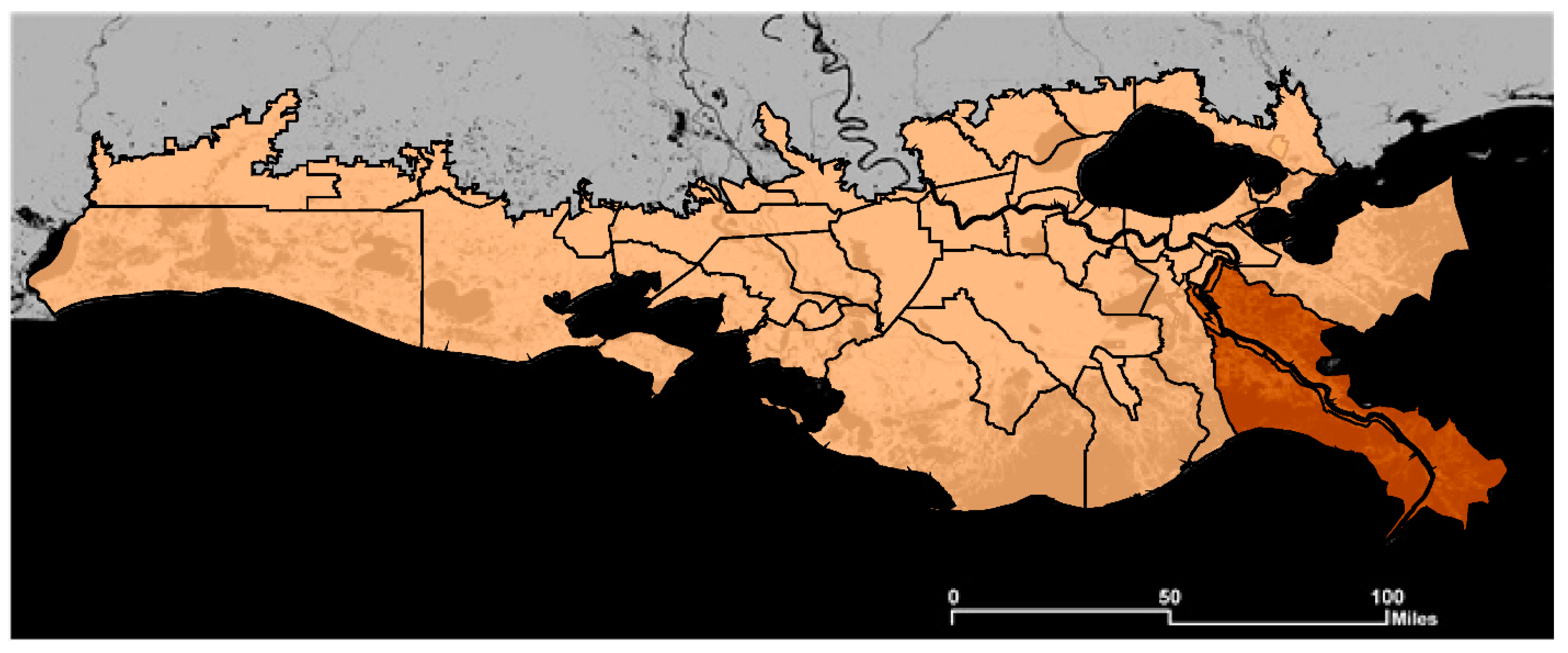
The full coastal Louisiana study region is shown in
Figure 1. For the purposes of Louisiana’s coastal Master Plan, the coastal zone is divided into 54 “risk regions” [
43]. These roughly correspond to regions defined by parish and then further subdivided by major bodies of water (e.g., the Mississippi and Atchafalaya rivers) or by protection features such as levees and floodwalls.
Figure 1 shows the risk region boundaries; highlighted in brown are four risk regions in Plaquemines Parish, for which we show illustrative results later on in the paper.
3. Results and Discussion
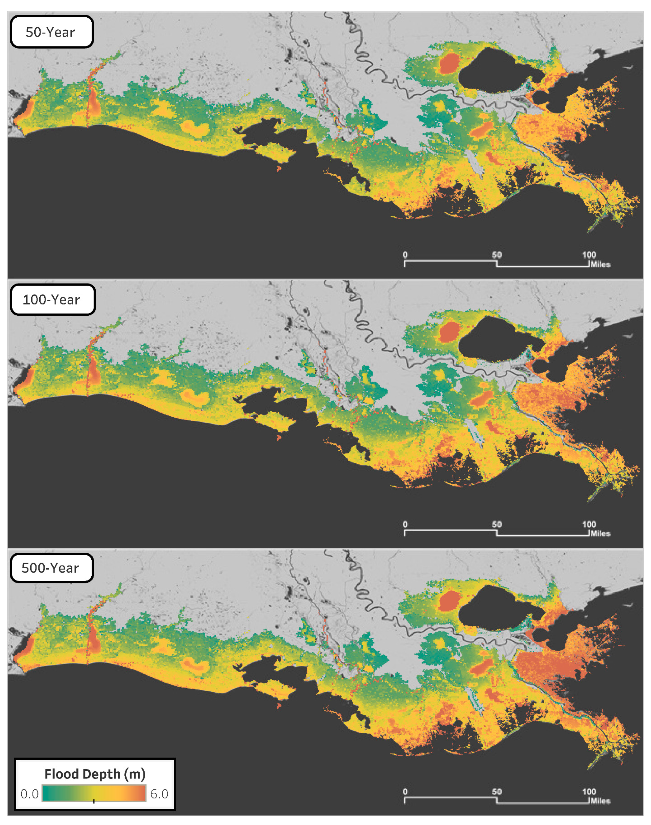
To understand the effects of updating our best estimates of the tropical cyclone mean inter-arrival rate and/or the relative likelihoods of synthetic storms using additional years of observed data, we compared the median estimated flood depths based on each truncated data set to the median flood depth exceedances calculated from all available data.
Figure 2 shows the estimated median flood depths for all three return periods of interest based on all HURDAT data from 1950 to 2016.
In large parts of the coast, 100-year flood depths exceed three meters, indicated by yellow or orange hues. While most of these areas are unpopulated wetlands or open water, this does indicate the potential for variability in best estimates to have substantial impacts on building codes for the new development or retrofits. Reducing flood vulnerabilities to such a high elevation above grade might require the first floor of buildings to be non-habitable space such as a garage or storage area [
44].
Comparisons with the median estimates displayed in
Figure 2 were made by finding the difference between the estimates from the full data set (1950–2016) and the estimates from each truncated dataset. Because the 1% AEP, “100-year,” flood depths are most commonly used to establish risk standards for insurance and policy purposes, we primarily focus on this particular return period.
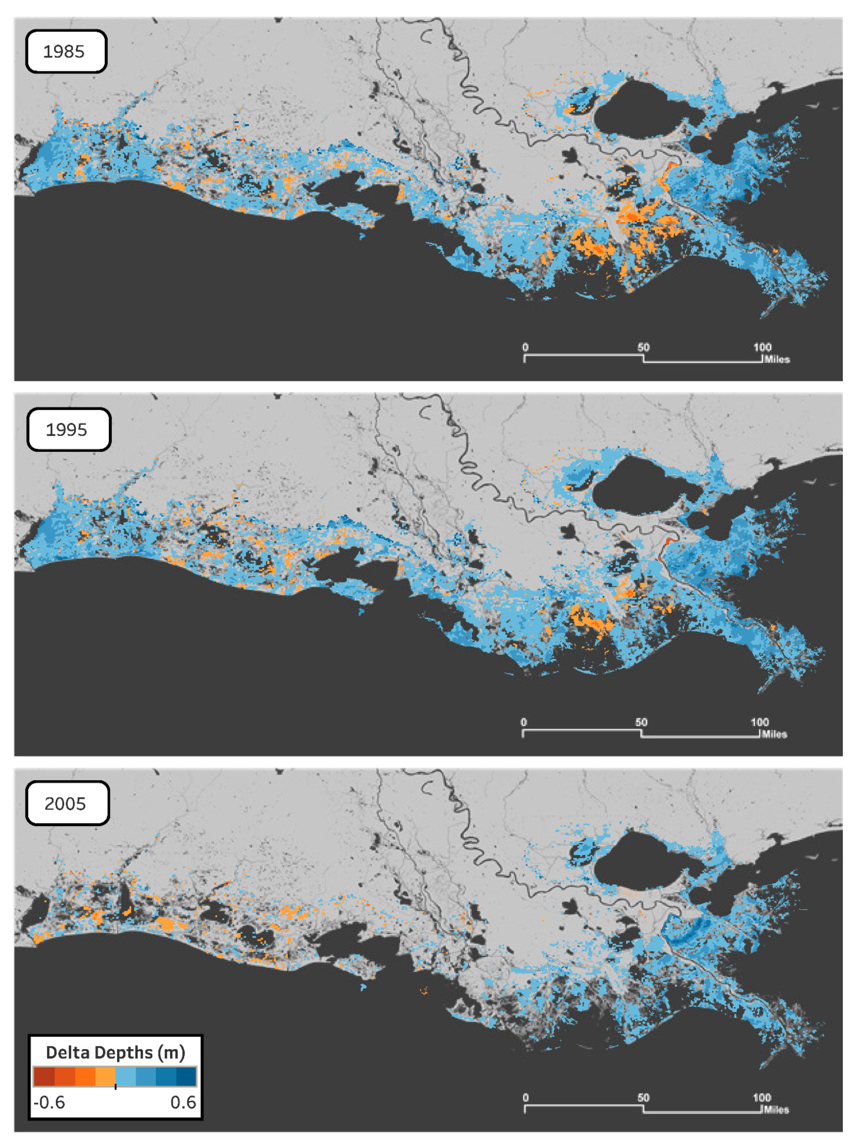
Figure 3 depicts the differences in the 100-year flood depth estimates for three years—1985, 1995, and 2005—as compared to the reference case ending in 2016. The values from the truncated case are subtracted from the reference values, so regions with positive values (blue) have greater estimated 100-year flood depths now in the reference case than a best estimate would have indicated in an earlier era. Alternatively, negative values (orange) indicate depths in the truncated case larger than the reference standard. This figure reflects estimates of both the mean inter-arrival rate and joint probability distribution using the truncated time series. Because of its importance in the regulation of critical infrastructure risk, we have also included a similar figure for the 500-year flood depths as
supplementary information (
Figure S3).
As seen in
Figure 3, there does not appear to be a region that consistently over- or under-estimates 100-year flood depths relative to the 2016 reference case. Although the comparison maps from 1985 and 1995 seem to overestimate in similar geographic regions, they are quite different from the comparison map from 2005, whose estimates appear to differ little from the 2016 estimates. Of course, we expect that differences will diminish as the truncated end year approaches 2016. While these individual years and the 100-year return period are not necessarily representative of the full set of calculated results,
Figure 3 indicates that variability in risk estimates may not exhibit systematic spatial or temporal patterns.
To further analyze possible geographic patterns, we examined differences in best-estimates within parishes
5 and between protected and unprotected communities. We can look at aggregate patterns of bias within the risk regions defined by the Master Plan.
Figure 4 summarizes the root mean squared deviation (RMSD) of 100-year flood depths, relative to the reference results, over all CLARA grid points located within the four risk regions comprising all parts of Plaquemines Parish (southeast of New Orleans and extending to the Gulf of Mexico) not contained within the Greater New Orleans Hurricane & Storm Damage Risk Reduction System (HSDRRS). Where
indicates the reference value for 100-year flood depths,
the best-estimate at grid point
in year
, and
the number of grid points in risk region
, the RMSD is defined by
As indicated in the legend, different lines indicate whether the mean inter-arrival rate (“frequency”), joint probability fits (“likelihoods”) or both factors were estimated using the truncated data set.
Supplementary Figure S4 depicts similar information at the 500-year return period.
Within Plaquemines Parish, best-estimates of 100-year flood depths within Braithwaite exhibit much more variation over time than other risk regions. The Braithwaite region is protected by a levee system, but it is not part of the federally-accredited HSDRRS and is not certified to provide protection against 100-year storm surge events. Our conjecture based on the analysis of flood depth exceedances in the reference case is that the region has 1% AEP flood depths close to zero, and non-linearities in overtopping and fragility mechanics produce a steep increase in the exceedance curve near the 1% AEP point. This results in a greater sensitivity in best estimates of 1% AEP depths to changes in assumptions about storm frequency or the relative likelihood of different types of storms when compared to regions that are either unprotected or have protection against greater-than-100-year surge events.
We also find a pattern that updating the joint probability fits only using the truncated data set (“likelihoods”) generally produces less deviation from the reference values than using the truncated data to update the underlying storm frequency estimate (or both parameters). This holds true in other risk regions not shown in
Figure 4 and suggests that best estimates of flood depth exceedances may be more sensitive to stochasticity in the estimated mean inter-arrival rate of storms than to variation in the parameters of storms that do occur.
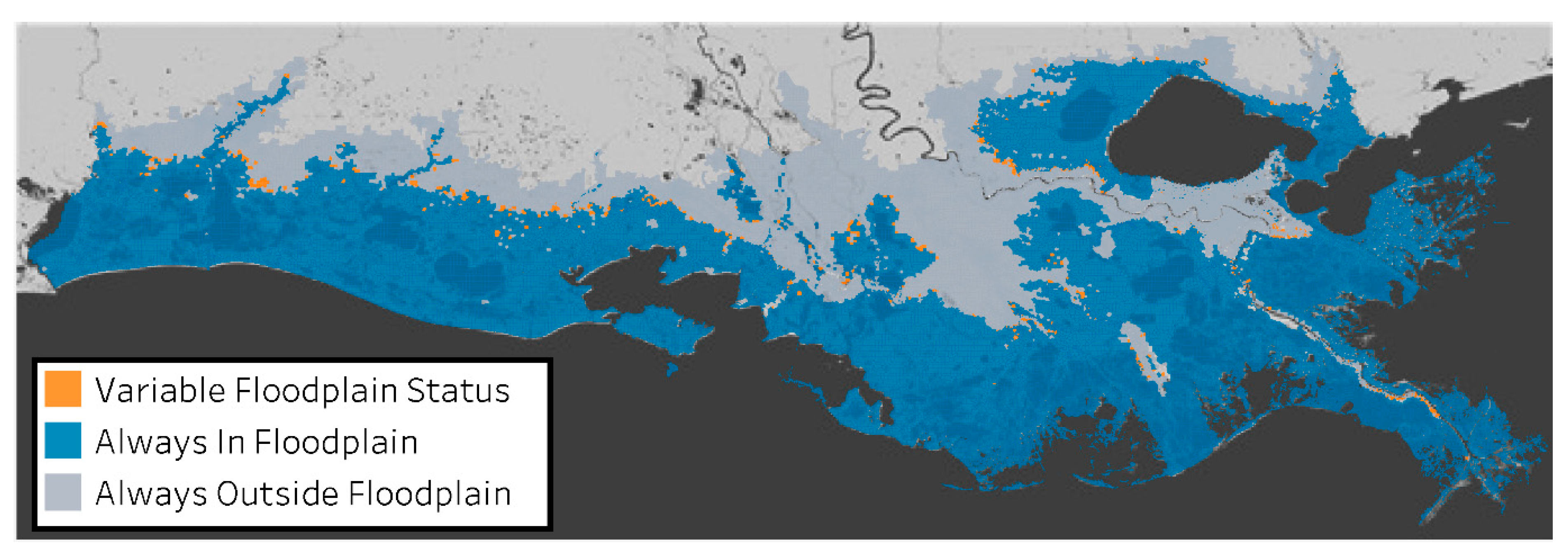
Although we did not uncover clear geospatial or temporal patterns to variation in flood depth exceedances, we can examine more closely how the evolving estimated 100-year floodplain
6 might impact the citizens of coastal Louisiana. After all, individuals who are determined by FEMA or another agency to be living within a 100-year floodplain are often required to purchase flood insurance or face other regulations on construction.
Figure 5 summarizes the estimated 100-year floodplain over each year from 1980 to 2016, showing whether a point is (i) always classified as being inside the floodplain, (ii) always classified as being outside the floodplain, or (iii) is classified as inside and outside of the floodplain in at least one year.
Supplementary Figure S5 shows the same demarcation of variability but at the 500-year return period.
As shown, the vast majority of coastal Louisiana’s land area is either always or never classified as being in the 100-year floodplain. However, for some portions of land in between these regions, their floodplain status varies as more storm data becomes available over time. For people living in this variable region, updating 100-year flood depth estimates more frequently might make a large difference in terms of whether or not they are required to have flood insurance.
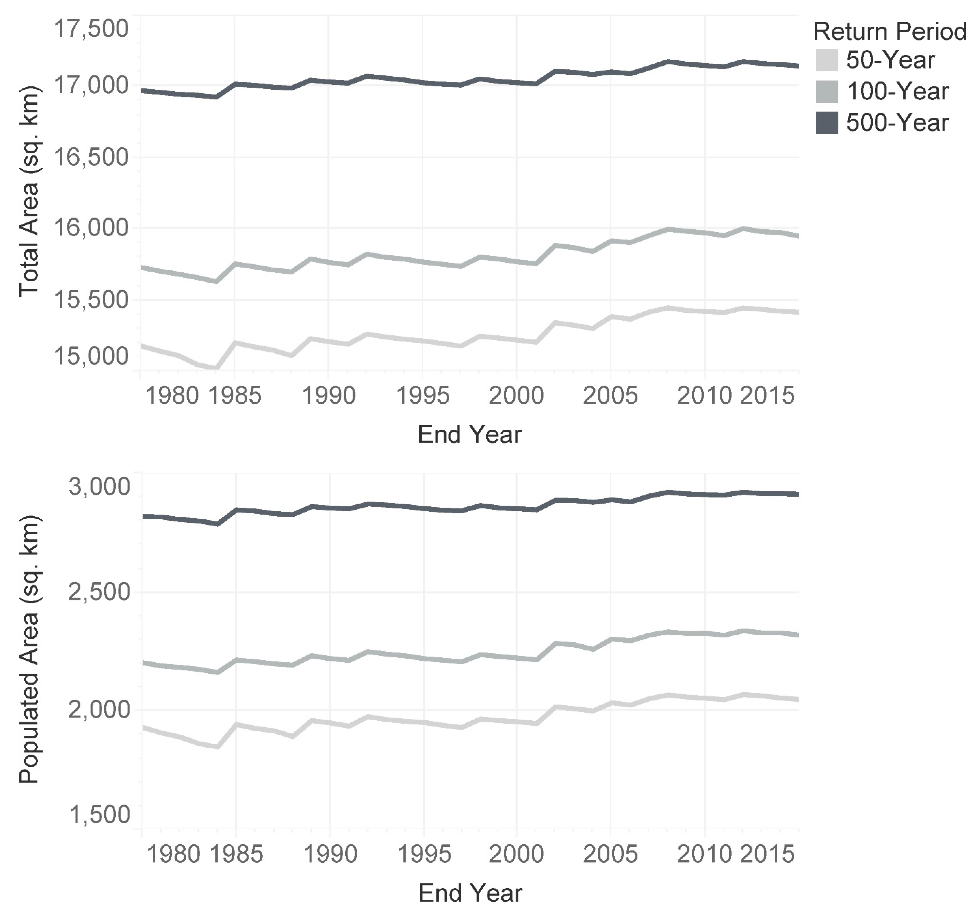
Figure 6 summarizes changes in floodplain extent at the 50-, 100-, and 500-year return periods. The top pane shows the total coastal land area classified as falling within the floodplain, while the lower pane shows the populated area within the floodplain
7. The actual values for each year and return period are provided in tabular format as
supplementary material. We see that some of the increases in floodplain extent correspond to years where storms made landfall, followed by gradual decays throughout subsequent years of quiet hurricane seasons in the Gulf. For example, the peak estimate of the 100- and 500-year floodplain extent occurred in 2012, when Hurricane Isaac hit. This observation is consistent with the finding that risk estimates are sensitive to the mean inter-arrival rate of tropical cyclones. Since 1980, the populated extent of the 50-year floodplain has grown by about 6%, the 100-year floodplain by 5%, and the 500-year floodplain by 3%. Uncertainty in the floodplain extent predicted by CLARA is shown in
supplementary figures that add confidence bounds for the 10th and 90th percentile estimates around the median values portrayed here (
Figure S1 for total land area and
Figure S2 for populated area).
Given the age of many FEMA-defined effective flood insurance rate maps (FIRMs) [
2]
8, this presents major implications for individuals living in these areas. They may have a mistaken impression of safety if misclassified as outside of the 100-year floodplain; alternatively, individuals misclassified as living within the floodplain may bear costs or regulations to which they should not be subject. Setting aside prescriptive questions about flood insurance and other policy mechanisms for risk management, this suggests that existing policies may not be implemented effectively.
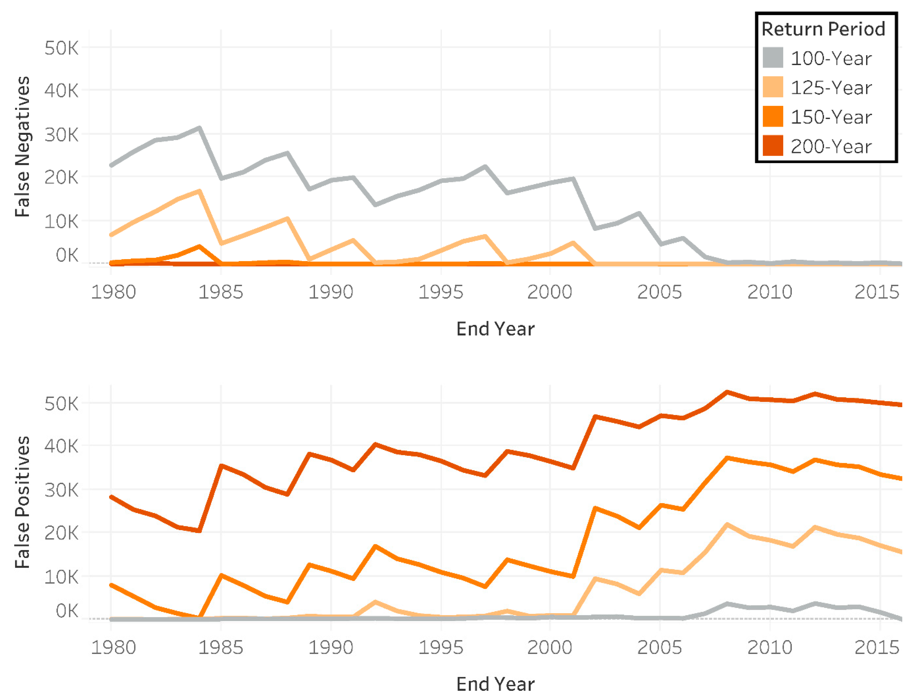
One possible way to address (i) the natural variation in the best-estimates of floodplain extent, (ii) the infrequency of updating estimates, and (iii) the trending growth in floodplain extent would be to use a lower-AEP floodplain to set policy. For example, when faced with an expanding and uncertain true 100-year floodplain, setting flood insurance requirements based on the best-estimate 125-year floodplain might allow for less frequent updates while maintaining the intended level of flood protection further into the future. To investigate this question, we tallied the coastal population that would be misclassified as being within or outside of the 100-year floodplain (relative to the 2016 reference standard) when using floodplains of various return periods based on a truncated time series. The results are shown in
Figure 7.
Two examples illustrating how to interpret this figure are as follows. In the top pane, the top line indicates that a 100-year floodplain defined in 1985 would result in about 20,000 “false negatives” in 2016: people classified as living outside the 100-year floodplain who really are inside a 2016 best-estimate. On the bottom pane, approximately 11,000 individuals who live within the 125-year floodplain, as estimated in 2005, would be classified in 2016 as “false positives,” in that they live outside of the 2016 100-year floodplain. As expected, the number of false negatives converges to zero over time, as all individuals living within the 100-year floodplain are eventually correctly identified with more data. However, as the best-estimate floodplains converge to their reference 2016 floodplains, the number of false positives associated with using less frequent AEPs to represent a future 100-year floodplain increases.
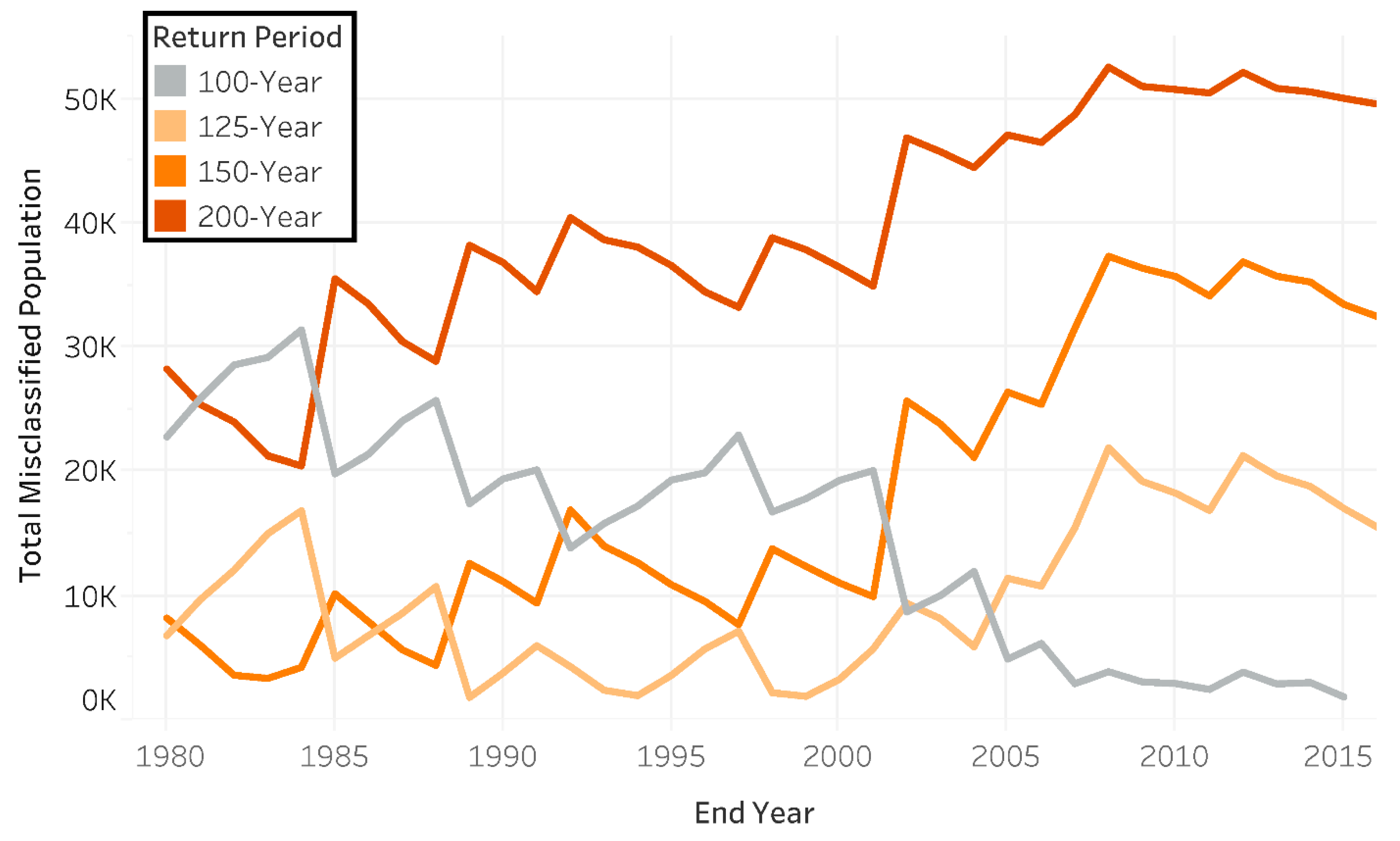
Consequently, as the floodplain grows, more people would be required to carry flood insurance. However, if flood risk estimates are not updated frequently, expansion of the floodplain might not be realized with enough time to ensure that these individuals are accurately informed of their risk. While false positives indicate that some homeowners are paying for flood insurance unnecessarily, houses incorrectly classified as being outside of the 100-year floodplain are at greater risk of experiencing flood damage without insurance. The total misclassified population is shown in
Figure 8.
Our analysis suggests that estimates of the 100-year floodplain may only minimize misclassifications for a duration of about 10 years, compared to floodplains defined by 125-year or less frequent return periods. This supports the existing guidance from the National Flood Insurance Reform Act of 1994 to “assess the need to revise and update all floodplain areas and flood risk zones” every five years [
45]. Decision makers with different preferences for avoiding false positives or false negatives, or those faced with another frequency of risk updates, may prefer to adopt a different strategy.

