Article

Real-Time Chronological Hazard Impact Modeling

1
Rhode Island School of Design, Providence, RI 02903, USA
2
Graduate School of Oceanography, University of Rhode Island, Kingston, RI 02881, USA
3
Department of Marine Affairs, University of Rhode Island, Kingston, RI 02881, USA
*
Author to whom correspondence should be addressed.
J. Mar. Sci. Eng. 2018, 6(4), 134; https://doi.org/10.3390/jmse6040134
Submission received: 7 October 2018 / Revised: 3 November 2018 / Accepted: 3 November 2018 / Published: 10 November 2018
(This article belongs to the Special Issue Coastal Hazards Related to Water)

Abstract

:
The potential of using ADvanced CIRCulation model (ADCIRC) to assess the time incremented progression of hazard impacts on individual critical facilities has long been recognized but is not well described. As ADCIRC is applied to create granular impact models, the lack of transparency in the methods is problematic. It becomes difficult to evaluate the entire system in situations where modeling integrates different types of data (e.g., hydrodynamic and existing geospatial point data) and involves multiple disciplines and stakeholders. When considering increased interest in combining hydrodynamic models, existing geospatial information, and advanced visualizations it is necessary to increase transparency and identify the pitfalls that arise out of this integration (e.g., the inadequacy of data to support the resolution of proposed outputs). This paper thus describes an all numerical method to accomplish this integration. It provides an overview of the generation of the hydrodynamic model, describes the all numerical method utilized to model hazard impacts, identifies pitfalls that arise from the integration of existing geospatial data with the hydrodynamic model, and describes an approach to developing a credible basis for determining impacts at a granular scale. The paper concludes by reflecting on the implementation of these methods as part of a Federal Emergency Management Agency (FEMA) Integrated Emergency Management Training Course (IEMC) and identifies the need to further study the effects of integrated models and visualizations on risk perception.

Graphical Abstract

1. Introduction

Hurricanes place critical facilities, such as hospitals, electrical systems, and transportation links, at risk [1]. The potential of ADvanced CIRCulation model (ADCIRC) as a tool to analyze vulnerabilities of specific geographic points has long been recognized [2]. This includes the potential for real time analysis of impacts and showing the chronological effects of a storm surge [2]. In this case, “real-time” refers to the ability to generate reports of hazard impacts (e.g., effects of the surge at an individual geographic point) as the underlying ADCIRC simulation is run or immediately after. “Chronological effects” refers to the ability to calculate hazard impacts for each time increment of the underlying ADCIRC model. Achieving a reliable real-time method to evaluate chronological hazard impacts at specific points may provide a new way to assess potential hazard impacts in the days and hours preceding landfall to adjust and improve preparation and response [2,3]. Researchers are also calling for improved methods for the integration of qualitative data into time incremented hazard impact models [4].
Methods to achieve the real-time connection of hazard impact models to ADCIRC are generally not elaborated in the literature. Methods for hazard impact modeling that have been elaborated largely rely on GIS software (e.g., ArcMap), and the effects are typically aggregated to show maximum possible impacts [2,5,6,7]. There is a recognition more generally that as modeling of phenomena, such as sea level rise, improves, that hazard impact models will need to be similarly improved to realize planning benefits for coastal communities [4,8]. There is also increased interest in integrating hazard impact models with visualizations that may display impacts to specific facilities (Figure 1) [9], and interactive 3D models for use in stakeholder engagement and on the web [10,11,12]. These integrations are distinct from methods that display inundation in such platforms as Google Earth, because they allow for highly individualized control of 3D assets (representations of structures, debris) [13].
This integration of different scales of data, disciplinary bases, and stakeholder concerns requires that systems be elaborated such that representational and modeling decisions may be scrutinized from multiple points of view (e.g., end user, ocean scientist) [14,15]. In the absence of such transparency, the relationship between the depicted hazard impact and the underlying technical information is unclear [16]. The process may be perceived as a black box and undermine confidence in the legitimacy of the outputs [17]. Describing methods by which time incremented granular hazard impact models are created thus becomes a necessary first step in developing rigorous, consistent, and transparent methods [14].
One means to create time incremented hazard impact models is to use an all numerical approach. This can be accomplished by using recording points that are built into the ADCIRC model, allowing for the interpolation of data at pre-selected locations [18]. This can also be accomplished with outputs of ADCIRC models (e.g., netCDF files) by indexing individual geographic points (e.g., representing an object or facility) to grid nodes of the ADCIRC model. In both cases, elevation data, such as ground elevation, inheres with the geographic point in a table with other necessary information to perform the analysis. This all numerical method makes it possible to program the hazard impact model in multiple programming languages that can be integrated with the ADCIRC model [18]. This allows for the hazard impact model to be run on the same platform as the ocean model, eliminating the “air gap” between processes. It further has the potential to eliminate errors of resolution that can result from transformations of data necessary to move ocean model data into geographic information systems (GIS).
The use of a method to evaluate individual points also raises questions. Hazard impact modeling often aggregates damages in terms of economic loss [4], or uses point data that was originally generated for other purposes (e.g., databases used by emergency responders such as e911 in the USA) [9]. While the application of these methods is appropriate over wider geographic regions to produce comprehensive and aggregated reports or risk maps [4,7], the application of statistically aggregated methods to derive outcomes for individual localized points becomes questionable [19]. Issues include the use of data of different types (e.g., point vs. areal) or derived at different scales [20]. This is in addition to problems that are associated with the imperfection of geographic data, or the impossibility of obtaining sufficient data for the intended purposes [21].
A point located at the centroid of a land parcel, for instance, may not reflect a specific vulnerability and could thus yield a false positive or negative (e.g., the facility in question is at lower or higher elevation than the point). To the extent that highly specific outcomes are predicted and potentially visualized using data made for other purposes, there is a danger that the certainty of outcomes is overstated and misleading [19,20,22]. The implementation of this approach thus requires careful attention to issues of data quality and the representation of outcomes.
This paper further elaborates the all numerical method for hazard impact modeling and approaches to contend with the questions it raises. It includes:
(1)
Overview of the storm surge modeling system, including: generation of the meteorological forcing, the hydrodynamic simulation model, and steps taken to validate the model using a historic storm (Hurricane Carol, 1954) and tide gauge data.
(2)
Architecture of the all numerical method, including steps taken to avoid errors of interpolation, or that might otherwise be introduced in more conventional processes by downscaling or the translation of data between data types (e.g., point, raster and polygon) [5,20,23].
(3)
Quality of spatial data, including issues such as positioning of geographic points to coincide with specific vulnerabilities to minimize errors resulting from use of data created for different purposes (e.g., e911) [19,20].
(4)
Participant input, including eliciting facility level vulnerability information as a credible non-aggregated basis for modeling specific impacts [7]. Developing highly specific granular data (e.g., the wind velocity at which a communication tower may be compromised) requires the engagement of stakeholders [4]. Incorporation of stakeholder input has been shown to increase the transparency of processes as well as enhancing trust and perceived legitimacy of model outputs [17,24].
The methods described were recently tested as part of developing time incremented hazard impact reports and visualizations to support a Federal Emergency Management Agency, Community Specific Integrated Emergency Management Course (IEMC) conducted by the Emergency Management Institute (EMI) and the Rhode Island Emergency Management Agency (RIEMA) in June of 2017. Where appropriate, examples that are used in this paper are drawn from this work. After expanding the four points above, this paper concludes with a reflection on the benefits of this work to the IEMC exercise and hazard impact modeling more generally.

2. Overview of the Storm Surge Modeling System

2.1. Generation of the Meteorological Forcing

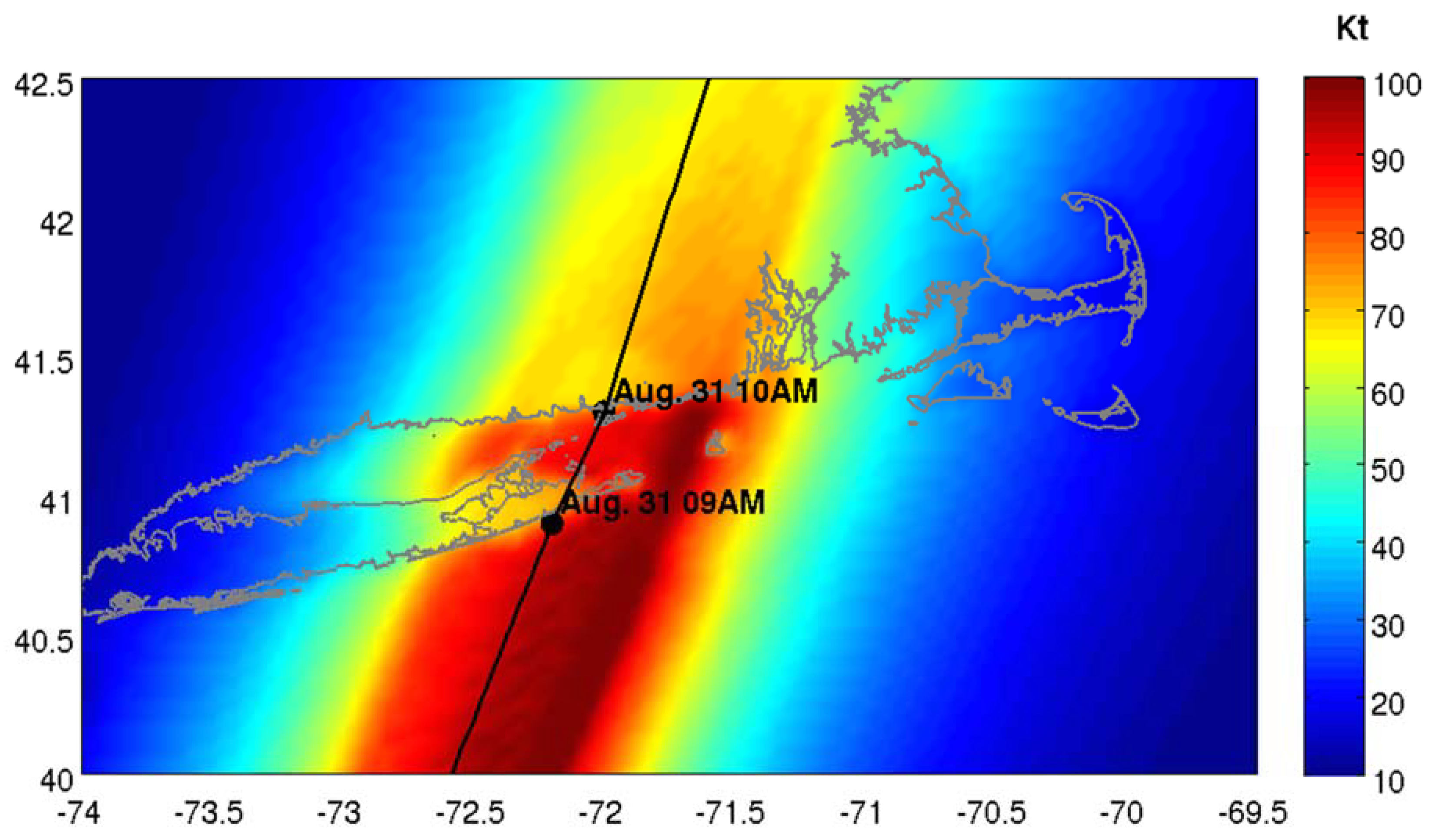
This study used a newly developed high-resolution hurricane boundary layer (HBL) model to provide physics-based simulations of surface winds during hurricane landfall. At landfall, the hurricane usually encounters a rougher surface with increased friction. The roughness length of the sea is of the order of a few millimeters, while land roughness lengths are typically several centimeters for open fields, and are greater for forested or urban areas. This change in the surface friction affects the near-surface wind structure. The hurricane boundary layer model, originally designed for open ocean hurricane studies [25,26], has been adopted for landfalling storms as part of the coastal resilience project at University of Rhode Island (URI) funded by the U.S. Department of Homeland Security (hereafter URI HBL). It is based on a dynamical approach that utilizes the physical balances in the dynamic equations to determine how a hurricane responds to local variability in the surface conditions (primarily topography and surface roughness). Figure 2 depicts an example of the coastal wind swath (maximum sustained wind experienced during the storm passage) that is produced by the URI HBL model for Hurricane Carol (1954), the most destructive hurricane to strike southern New England since the Great New England Hurricane of 1938. The National Weather Service in Warwick, Rhode Island recorded sustained winds of 90 mph, with a peak gust of 105 mph.
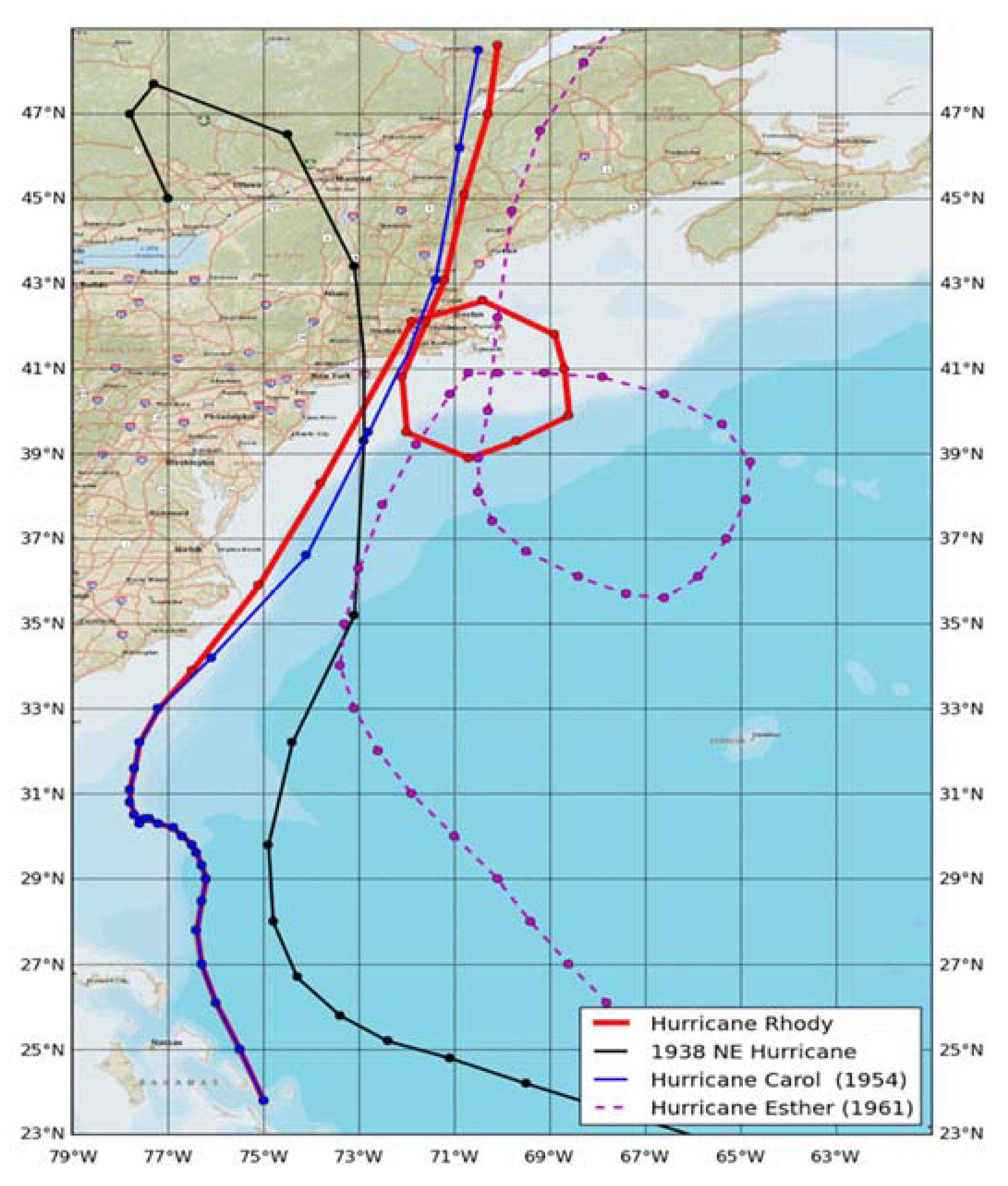
A hypothetical yet plausible hurricane scenario was created to simulate the effect of a high-impact storm in Rhode Island named “Hurricane Rhody” (Figure 3). This scenario involves a major hurricane that starts near the Bahamas and propagates northward close to the U.S. East Coast. While staying close to the coast (like Hurricane Carol in 1954), it moves much more quickly (like the Great New England Hurricane of 1938). Ultimately, the storm makes landfall in central Long Island and then in Connecticut (like the hurricanes of 1938 and Carol), as a strong Cat 3 hurricane with peak winds of 132 mph causing a huge storm surge in Narragansett Bay and along the south shore of Rhode Island. Then, shortly after its landfall near Old Saybrook, Connecticut, the storm slows down, stalls, and loops over Southern New England, which is somewhat similar to Hurricane Esther in 1961. Rhody makes the second landfall as a Category 2 hurricane in Rhode Island, producing strong winds and heavy rainfall. The total rainfall reaches more than 25 cm in some areas, causing massive river flooding, similar to Hurricane Diane (1955) and the Rhode Island March 2010 floods.

2.2. Hydrodynamic Simulation Model

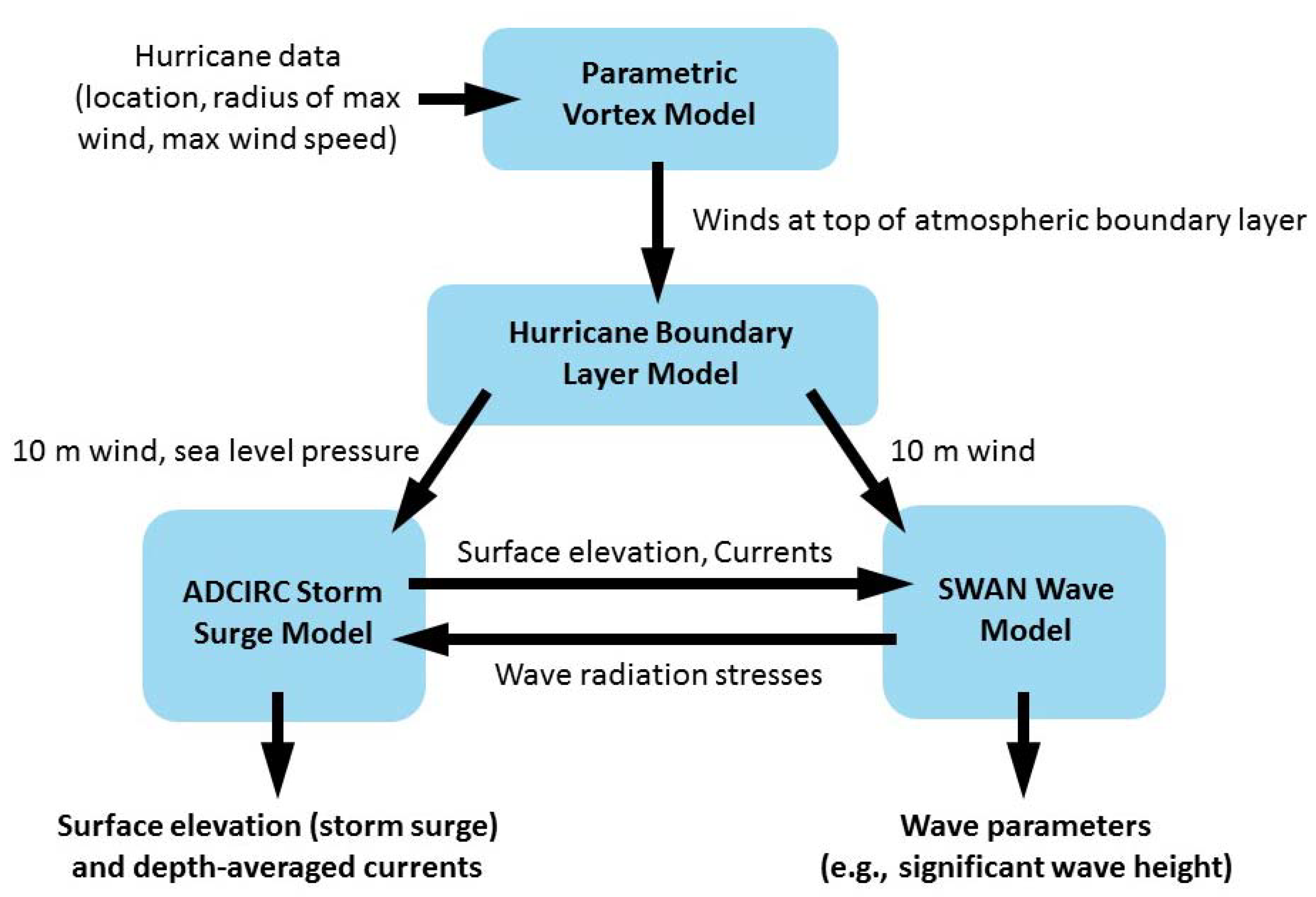
Storm surge response to the modeled hurricane wind and atmospheric pressure fields was computed using the ADCIRC model coupled with the Simulating Waves Nearshore (SWAN) model (Figure 4). ADCIRC is a finite element model that, in the 2-dimensional mode employed here, solves for water level using the generalized wave continuity equation (GWCE) and depth-averaged current using the shallow water momentum equations [18]. SWAN is a third-generation, phase-averaged wave model for simulating wind waves in coastal and open ocean regions [27]. ADCIRC and SWAN are coupled by passing the wave radiation stress computed from the SWAN wavefield to ADCIRC and passing the water levels, currents, and frictional parameters from ADCIRC to SWAN [28]. Both models are run on the same unstructured mesh using triangular elements. Further details of the storm surge simulation model are described in Dietrich 2011 [28].
The unstructured model mesh covers the northwest Atlantic, the Caribbean Sea, and the Gulf of Mexico with an open boundary at the 60° W meridian. It provides highest spatial resolution in key areas of interest and lower resolution in other areas, with triangular elements of the order of 50–100 km in size over deep ocean areas, decreasing to the kilometer scale over the continental shelf. The mesh is highly refined in the region of interest (southern New England), where element sizes decrease further to 30 m along the coastline. The mesh extends inland of the coastline, to the 10 m elevation contour, in order to enable the simulation of overland inundation. The Fox Point Hurricane Barrier, constructed in Providence after devastating flooding during the 1938 hurricane and Hurricane Carol in 1954, was represented in the model mesh as a weir (dam) with a height of 7 m. The height of 7 m and alignment of the barrier was verified using LiDAR elevation data.
A key input to any storm surge model is the bathymetry/topography of the region to be simulated. The bathymetry/topography of the Rhode Island region was interpolated from a digital elevation model (DEM) of the area that was provided by the Rhode Island Geographic Information System (RIGIS) with the vertical reference datum converted from NAVD88 to mean sea level (MSL), which is the natural datum of an ocean model. This adjustment, based on the NAVD88-MSL difference at the National Ocean Service tide gauge at Newport RI (NOS station 8452660), was 0.093 m.
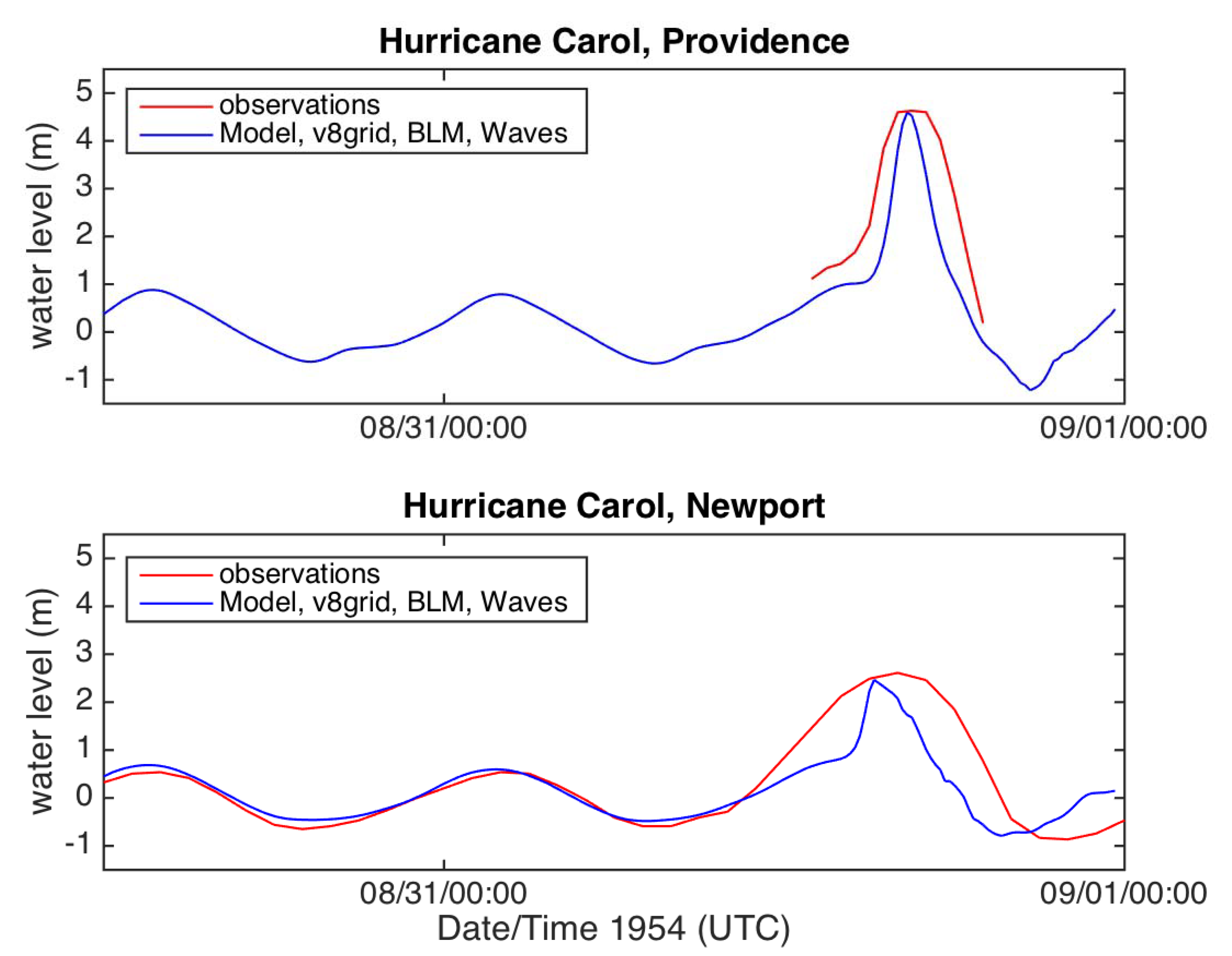
The coupled ADCIRC/SWAN modeling system was verified in the Rhode Island region with a simulation of Hurricane Carol, which impacted the area in the late summer of 1954. The water level time series from this simulation, which was performed using a mesh lacking the Hurricane Barrier that was not present at the time, were compared to observed water levels at Providence and Newport (Figure 5). The results indicate that the model accurately simulates the maximum water level during the storm surge, but that the duration of the model surge is too short relative to the observed storm surge. The reason for this is likely imperfect model wind forcing at the edges of the hurricane where the interaction of the hurricane and the mesoscale meteorology are not captured.

3. Architecture of the All Numerical Method

3.1. Overview

Parallel of the HBL wind model and hydrodynamic simulations, the URI Department of Marine Affairs (MAF) has been developing hazard impact modeling and visualization methods that are based on the previously described all numerical method for connection to underlying models. Although this paper focuses primarily on connection to ocean models, such as ADCIRC, the fundamental architecture can be applied to wind models or other simulations. Using these methods, geographic points representing specific pieces of infrastructure are indexed directly to multiple nodes of the simulation [13].
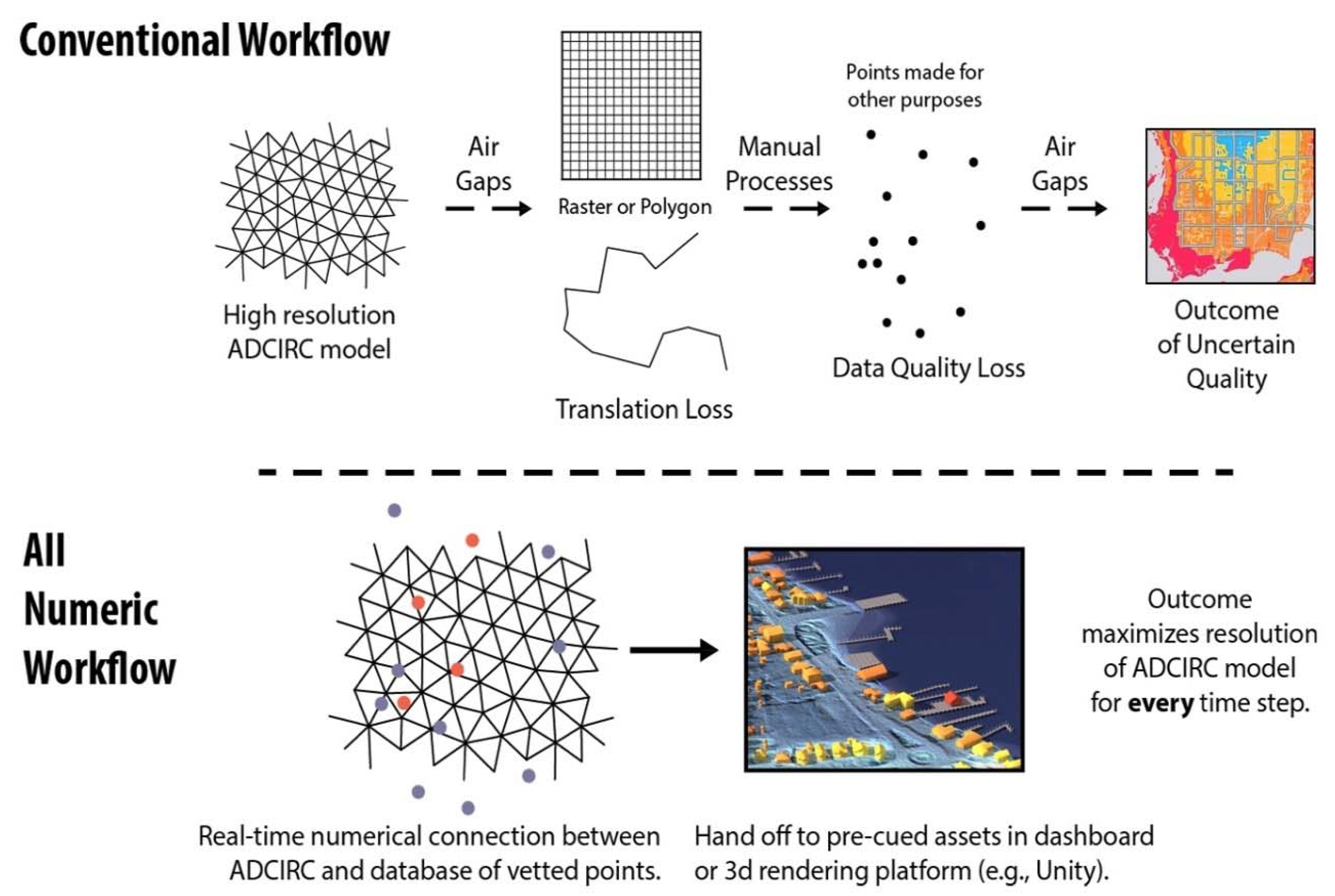
Traditional GIS workflows typically involve transforming outputs of the ADCIRC or other model into raster maps or polygons that can be compared to geographic points using ArcMap or other applications (Figure 6). Depending on how this is accomplished, such procedures may involve multiple manual steps for each timestep tested, or the compilation of maximum values. By contrast, the all numerical method pre-indexes each geographic point to nodes of the ADCIRC model (methods for interpolation are discussed in the next section). This indexing allows for the values from the ADCIRC model to be associated with the geographic point, and for operations (calculating inundation depth at the point for instance) to be carried out continuously for each point for every time step without manual intervention.
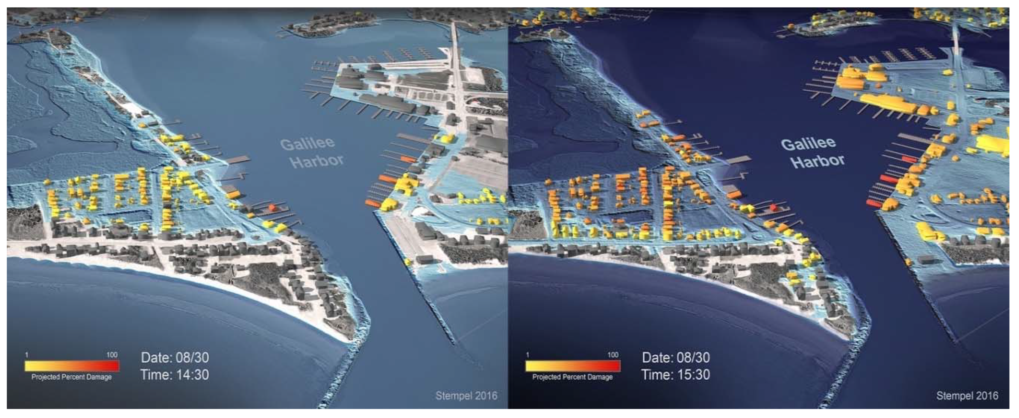
The initial implementation of the all numerical method tested structures in the area around Galilee, Rhode Island, USA, and implemented damage functions developed by the U.S. Army Corps. of Engineers as part of the North Atlantic Coast Comprehensive Study [29]. Once indexed to the unstructured grid, the structures and visualizations of those structures could be automatically updated based on adjustments to the model run, or tested against other storms (e.g., Hurricane Bob) that was run on the same grid (Figure 7). In addition to cataloging attributes of structures, extensive data was gathered for testing of debris objects and infrastructure, such as electrical transmission poles.
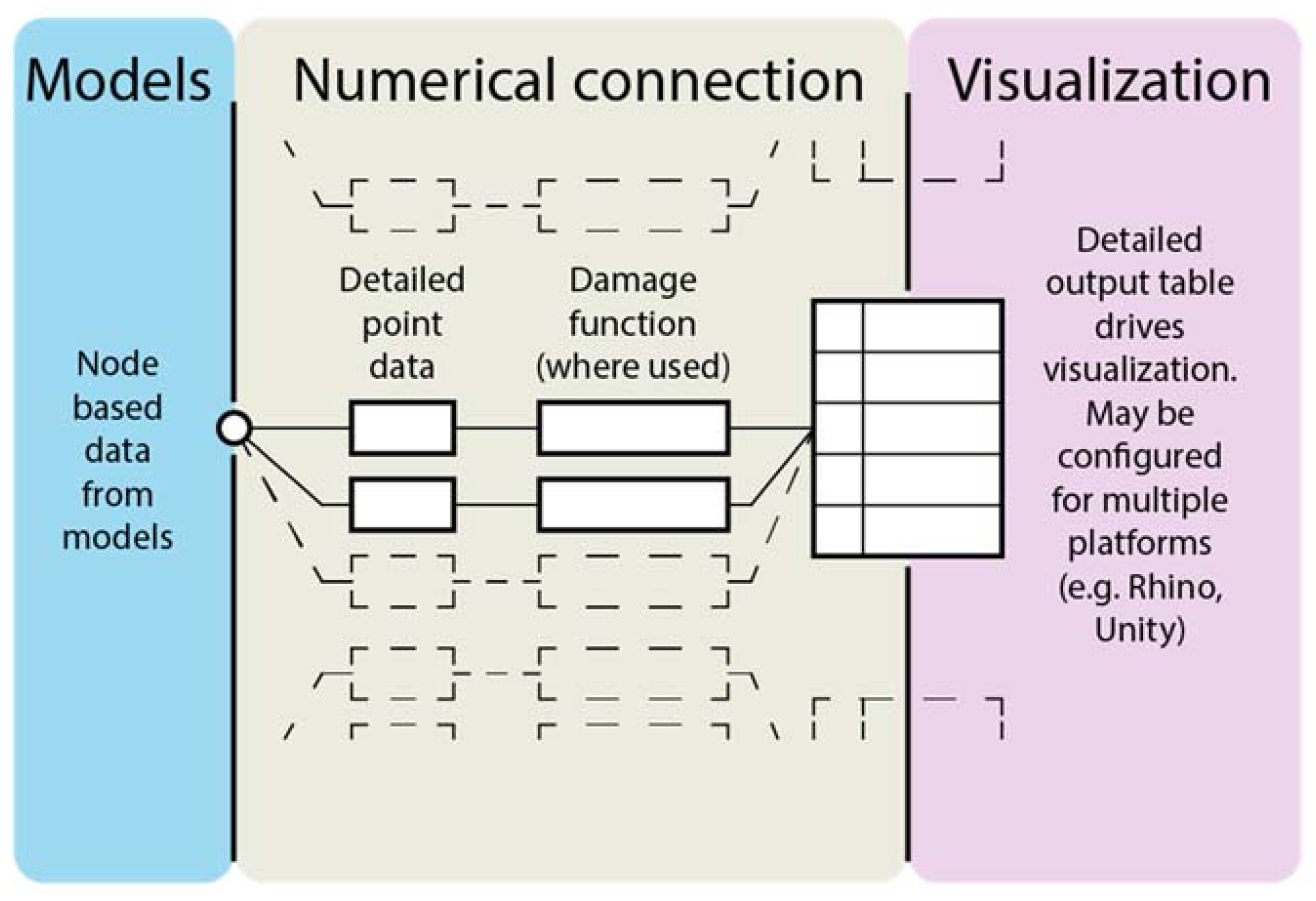
The fundamental architecture used to depict Galilee, Rhode Island USA, formed the conceptual basis for developing the all numerical method into a rapidly updatable method for hazard impact modeling. Outputs from the hazard impact models are formatted to drive visualization and rendering platforms, such that outputs may control the pre-established 3D model content. This approach is suitable for any platform that allows script-based placement and or control of 3D Assets. Examples of rendering platforms include Rhino 5 (McNeel and Associates, USA) and Unity (Unity Technologies USA). Simpler outputs may include dashboards, or, in the case of the IEMC, time incremented tabular impact reports (Figure 8). A key improvement of this method to drive visualizations over past methods is that the determination of outcomes is a transparent part of the modeling process, allowing for output tables to be scrutinized apart from the visualization (rather than being embedded in the technically complex and opaque visualization processes) [19,30].

3.2. Interpolation

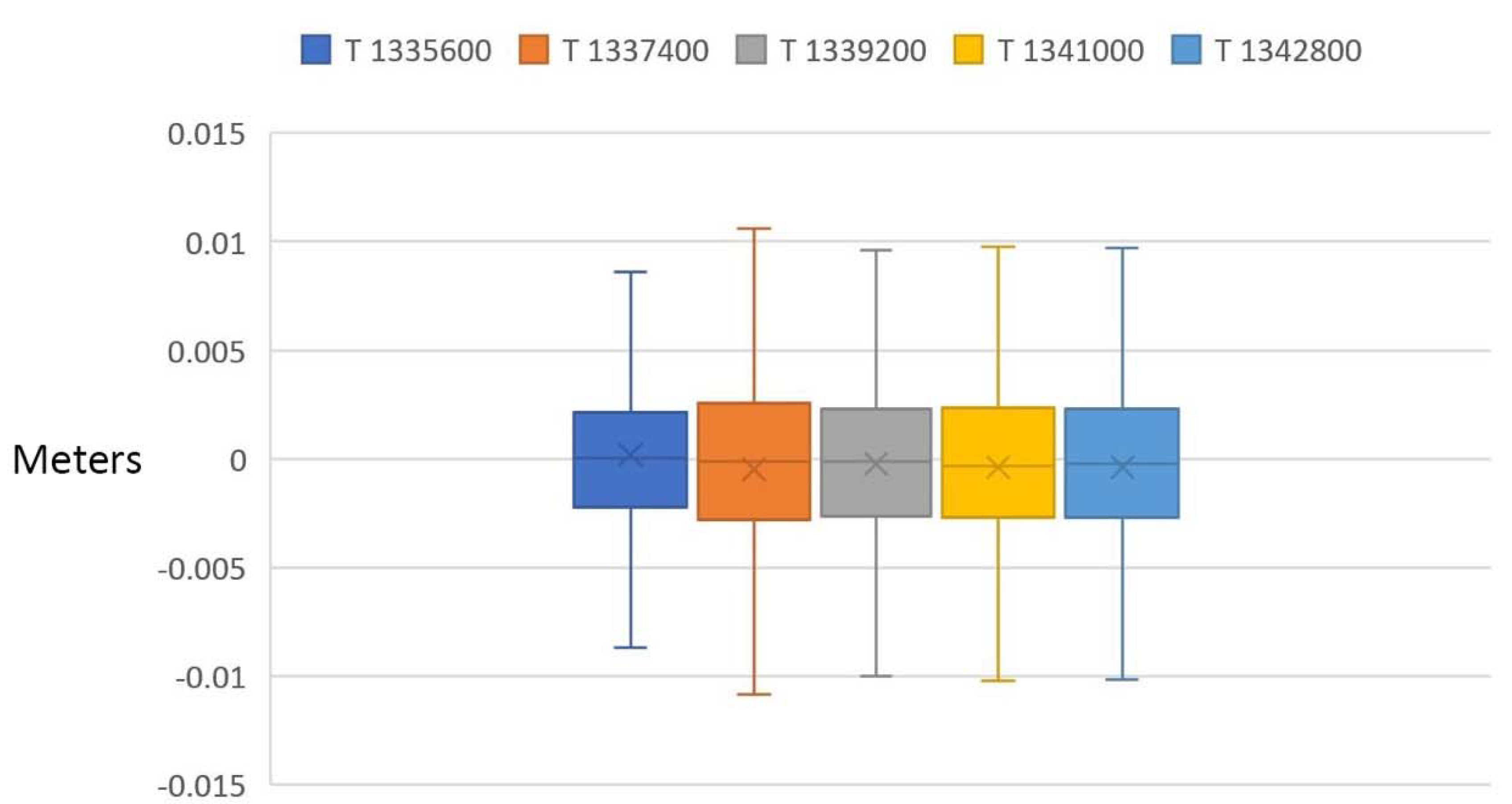
The fundamental innovation of the all numeric method is relating the geographic point and its attributes directly to the sea surface, as described by the unstructured grid. ADCIRC contains an inbuilt function to interpolate sea surface elevation at preset recording points [18]. When this is accomplished using outputs of the ADCIRC model (as opposed to direct integration), interpolation may not be necessary. The advantage of not using interpolation is speed of analysis over multiple timesteps on a laptop or desktop computer. As an example, a sensitivity test was performed in an area of concern in analyses, the Fields Point area of the Port of Providence. This analysis entailed testing the first, second, and third nearest neighbors of 12,176 nodes. The horizontal distance ranged between 22.8 m apart and 73.9 m. The variation reflects the optimization of the unstructured grid to fit the topography (e.g., greater node separation where less detail is required).
Most adjacent nodes vary by less than 0.003 m. The maximum variation between adjacent nodes in the sample set is 0.015 m (Figure 9). Given the small variation between relevant nodes, interpolation is not required. Similar tests in other sites yielded similar results. The maximum variation between the nearest nodes across the State of Rhode Island for these timesteps is 2.47 m, reflecting adjacent nodes in Block Island Sound.
Interpolation, where necessary, may be accomplished by indexing the geographic points to multiple adjacent nodes and using geometric interpolation. The indexing and associated interpolation or extraction methods include:
(1)
Geographic point with three adjacent wet nodes (nodes which are reported to be inundated by the ADCIRC model): interpolate sea surface elevation, water direction, and velocity based on the geometric relationship of the point to the planar surface described by the three points.
(2)
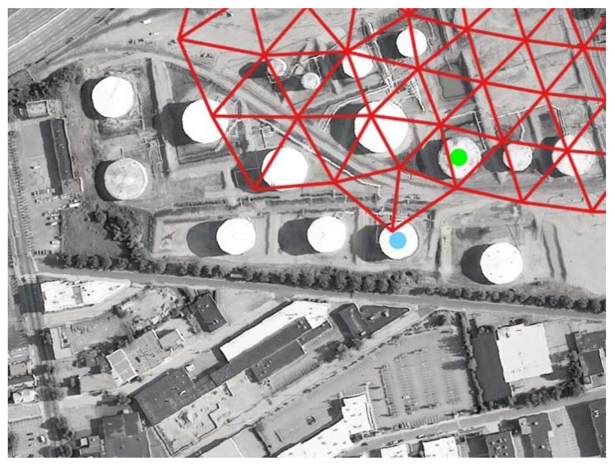
Geographic point beyond the last wet node: use nearest adjacent node without interpolation (Figure 10).
This interpolation method presumes that sea surface is described by the z of each node as a Delaunay triangulation. This is the optimal triangulation for the unstructured grid and is thus identical to the ocean model grid with the exception of reflecting z elevation of the water surface [31]. The interpolated value is understood to be measured where it intersects with the plane described by the three points. Interpolation between node points is thus optimized for each geographic point based on the available data [32]. The evaluation of points beyond the model grid accounts for situations where small-scale topographic conditions would cause inundation to extend beyond the last wet point of the ADCIRC model. All points are constrained by a basin analysis, such that points outside of the basin are not included. Vertical data, such as LiDAR derived ground elevation, inheres with the geographic point. Registration is accomplished by referencing a common datum, in this case, NAVD88 with a correction for the previously described discrepancy between MSL and NAVD88.
The use of this method avoids compromises in speed and resolution associated with the translation of node-based data into raster maps. It allows for outcomes for multiple timesteps to be easily determined and updated and preserves the elevation of the sea surface. Determining whether points are inundated based on transforming the wet portions of an ADCIRC model into a polygon defining inundation extent, by contrast, effectively transforms the middle areas of the simulation into a bathtub model (geographic points wet or not wet), even if the edges of the polygon capture elevation variation (e.g., if the polygon is determined through the comparison of two raster maps). In locations where there is significant change of geography, such as the narrowing of a river, the elevation of sea surface can vary by measurable amounts, even in small geographic areas (Figure 11).
Additional data, such as finish floor elevation of a structure, freeboard (clearance to vulnerable portions of a structure) details of its construction, or the presence and elevation of protective barriers, such as flood walls, inheres with the geographic point so that all calculations that are relevant to its involvement may be accomplished in a single process. Hazard impact assessments that are made with this method may thus combine a high degree of intricacy with speed, and potential improvements in resolution associated with interpolation.

4. Quality of Spatial Data

The improvements to resolution and intricacy referenced above are highly dependent on the quality of underlying data. A fractional improvement to methodology is meaningless if there are gross errors in underlying points. The resolution of data often depends upon the purpose for which it was created [20,21]. Developing highly specific predictions based on generalized data that has not been vetted for that purpose is thus problematic, and it can create misleading results that imply a level of precision that is not supported [19,20]. Ground truthing of geographic points, a process of determining whether point data is sufficiently detailed or accurate, is thus essential if highly specific predictions are to be made.
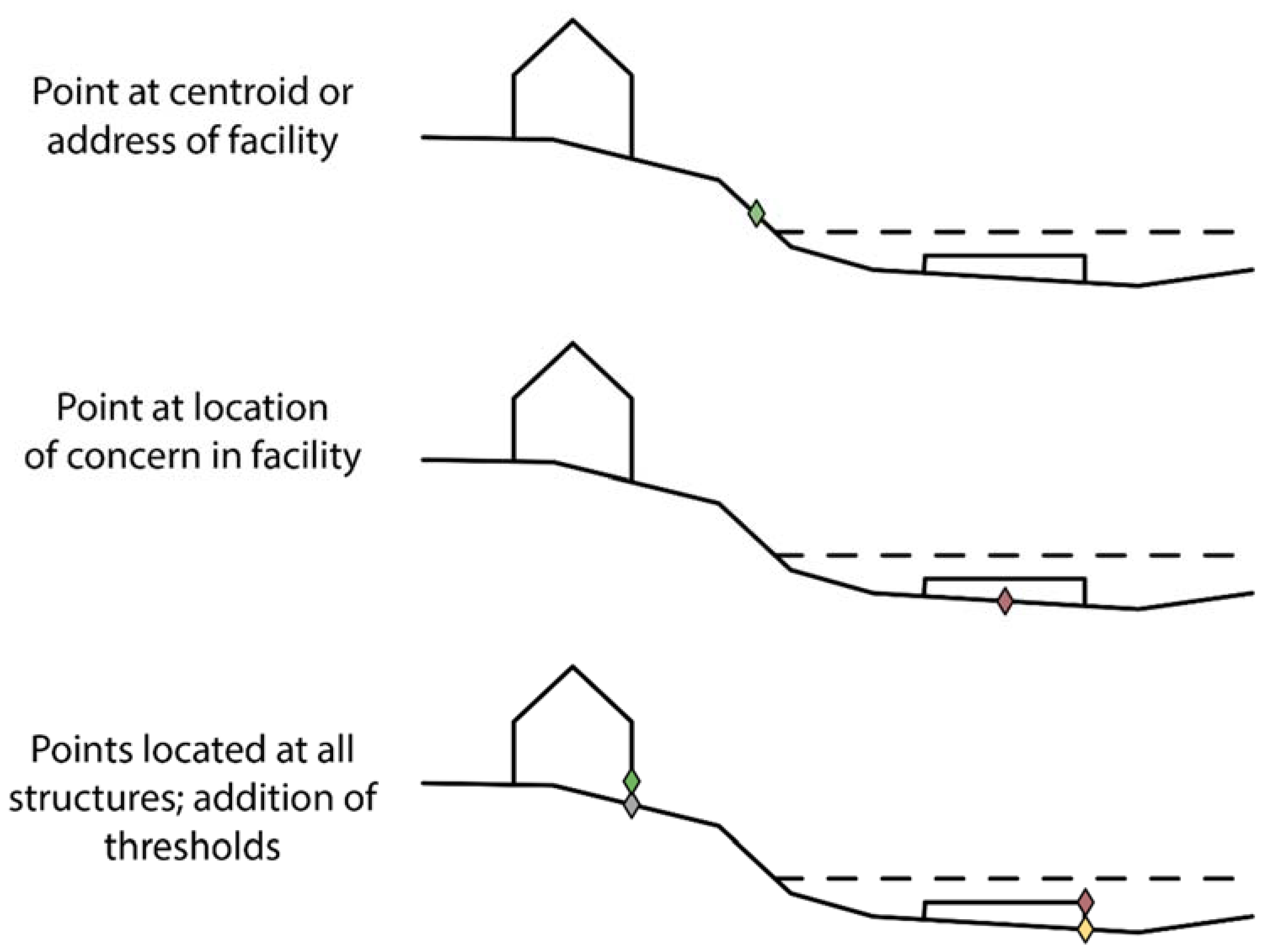
Points that are associated with databases made for other purposes, such as e-911 databases, while sufficiently accurate at geographic scales, might have limited utility at granular impact modeling scales. A single point representing a wastewater treatment facility, for instance, may be located arbitrarily or at the centroid of the land parcel that the facility occupies. The elevation of this point may be at a significantly different elevation than vulnerable portions of the facility. Moreover, facilities may include multiple vulnerabilities with distinctly different hazard exposures (e.g., inundation vs. wind). For this reason, individual points in here to individual structures within a facility, or minimally, are located based on vulnerability (Figure 12).
A sensitivity test comparing elevations of existing point data (obtained from Rhode Island GIS, e911, and Department of Homeland Security Office of Cyber and Information Security) was performed to compare the existing points used in analyses (e.g., points marking structures or the centroid of the property) with the elevation of the vulnerability (e.g., a clarifier that will be damaged if water exceeds an elevation). This analysis revealed the difference between the lowest existing point and the lowest point of vulnerability had a mean of 2.33 m. In the analysis, the least elevated points for each site were compared with least elevated vulnerabilities, and most elevated points were compared with the most elevated vulnerabilities (Table 1). Thus, this assumes that, when existing points are used in an analysis, that the “worst case” is utilized. Had highest been compared to lowest, the variations would have been more extreme. Waste water treatment facilities, which employ gravity as part of processes, often feature elevation changes on site, and are therefore acute examples, however they are not unique.
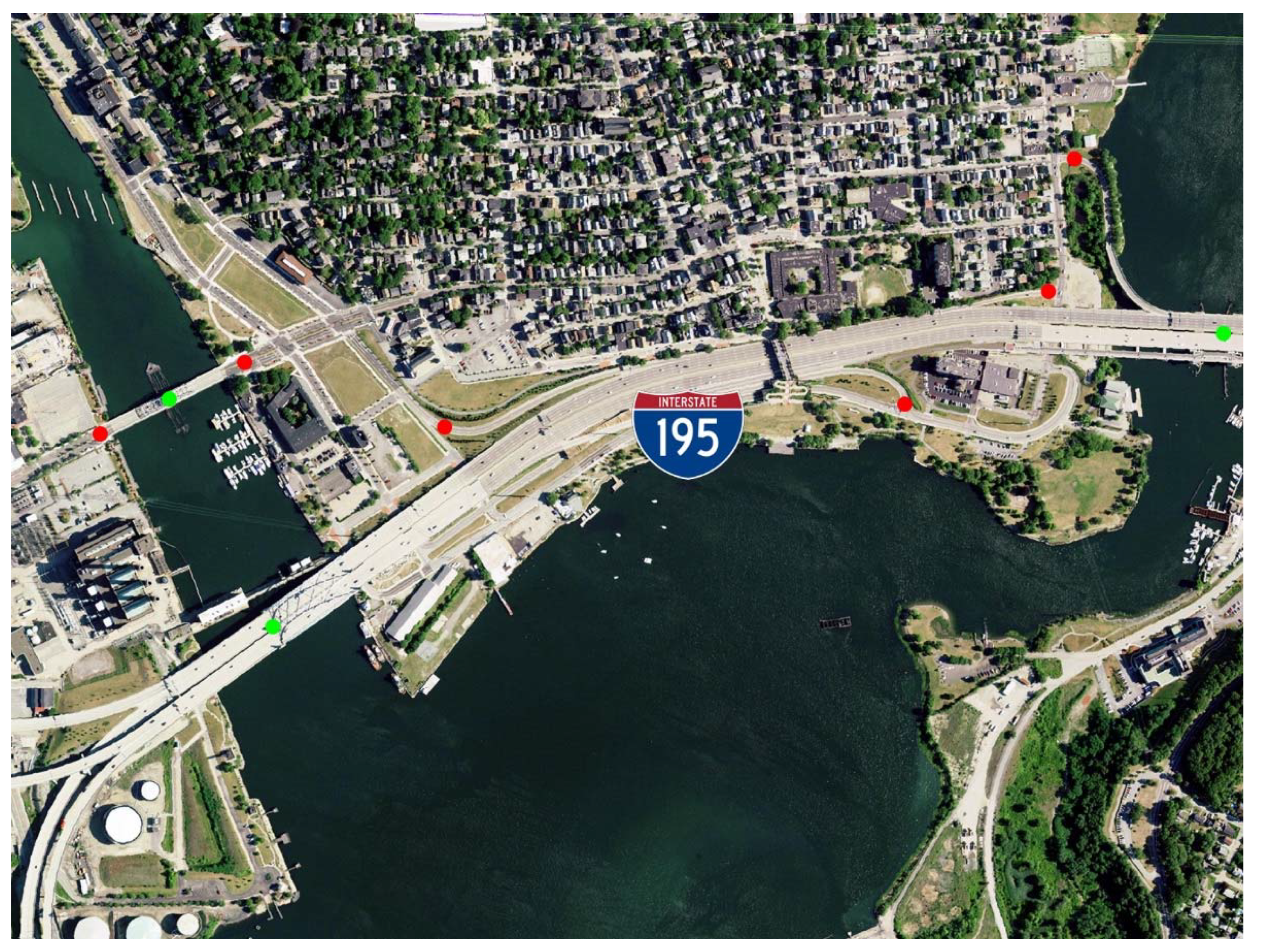
Bridges similarly create complex analytical problems, as they are subject to multiple forces (e.g., scour, shear) [32,33], and they often involve structures at multiple elevations. Representing a bridge as a single point is therefore problematic. In addition to the question of structural damage, there is a larger question of the role that the bridge plays in emergencies in providing access. For this reason, special attention was paid to the elevation of highway access points in analyzing data for the IEMC (Figure 13). These access points play a significant role in the transportation to and from a major hospital.
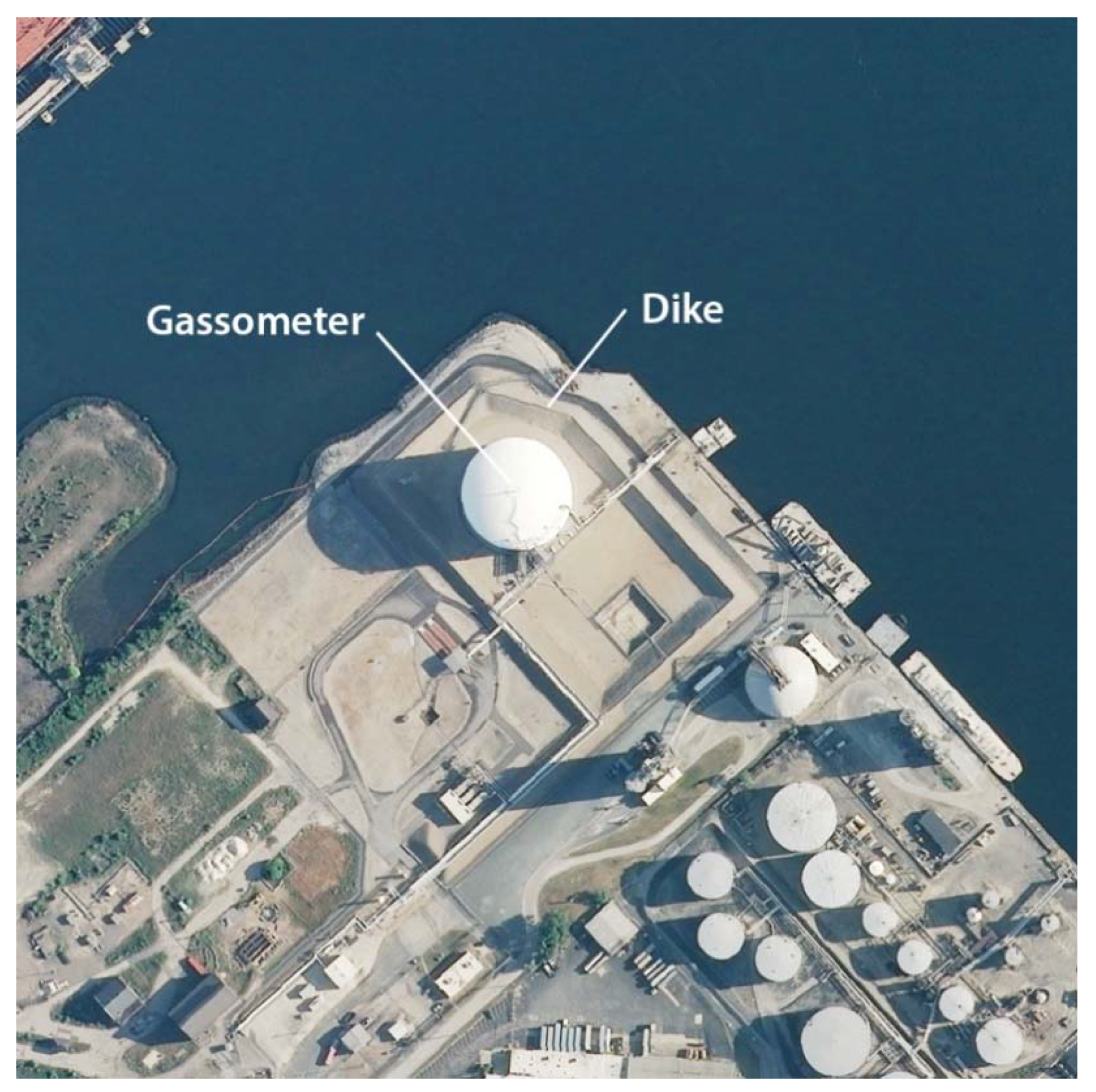
Ground truthing is also necessary where micro-topographical conditions are invisible to the ocean model. Such is the case with armored concrete reinforced protective dikes that surround liquified natural gas storage tanks in the Port of Providence (Figure 14). These types of conditions have necessitated the development of special attributes within databases that were developed for the IEMC and other projects. The presence of these dikes, including the threshold at which they are overtopped, is included in the point data representing the tank. Although wind damage to petroleum storage tanks was not specifically modeled for IEMC, these facilities serve as a primary example of points that can have multiple damage modes (e.g., buoyancy, wind damage) [34], and thus may require data for multiple analyses.
Beyond obvious issues of accuracy that are associated with using granular data, attention to observed conditions likely plays a significant role in the perceived credibility of visualization outputs [35,36,37]. To the extent that abstract simulations like ocean models are treated as equivalent to reality without sufficiently accounting for these conditions there is a danger that inconsistencies between the model outputs and observed reality undermine the credibility of the models when they do not agree with observed reality [38].

5. Participant Input

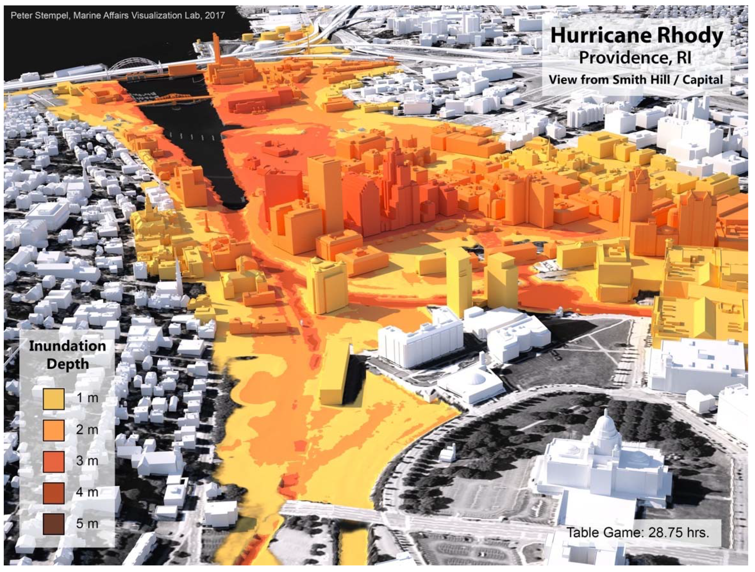
Issues of data quality point to larger concerns that are raised by detailed hazard impact modeling and especially visualizations. Namely, such models do not account for the compounding of uncertainties (e.g., natural and physical interactions and human responses that are not modeled) [22]. Moreover, the production of highly realistic visualizations crystalizes outcomes and implies higher degrees of knowledge and certainty than models may support (Figure 15) [22]. It is thus necessary to consider these effects in the application of visualizations, so as not to mislead audiences. In this case use of hazard impact modeling and visualizations were limited to the IEMC and participating experts [22].
The role of experts in developing and using hazard impact models for disaster risk reduction is widely recognized. Their contributory role is specifically cited in the recommended methods for developing impact models beyond basic models as part of the Hazards US model (HAZUS) [7,39]. As previously argued however, there are logical questions regarding the application of generalized statistically derived damage curves to highly specific structures. Even in situations where appropriate ground truthing has taken place regarding the geometry of a vulnerability, the application of a generalized curve may not be appropriate. The description of highly specific outcomes that are based on vague data, for instance, can make highly uncertain outcomes appear certain [22]. This issue was particularly concerning as it pertained to the IEMC because of the need for highly specific outcomes (e.g., disruption of a generator or communication tower) to be reported as prompts used during the exercise.
To address this, a process to engage emergency managers was initiated at the outset of the process in collaboration with RIEMA. This process enlisted local emergency managers in the development of model inputs that would be used in generating the hazard impact models. These inputs primarily included the development of a “thresholds database” that included specific facilities of concern and quantifiable thresholds at which described outcomes could be expected.
The concept of using thresholds or triggers to define inter-related impacts of storm events is drawn from approaches to planning that seek to organize responses to uncertain future conditions and interdependencies [40,41,42]. In these planning processes, thresholds are identified for different levels of future hazards to assess future vulnerability [40,41]. As it pertains to the methods that were used by URI, quantifiable triggers related to measurable effects of wind, rain, and inundation were collected to be used as model inputs to be tested against storm scenarios and incorporated into databases tested against the relevant models. Where multiple factors contributed to a specific impact (e.g., the combination of wind and ground saturation from rainfall), connection between models was made manually. In future iterations, it is conceivable that such hand offs could be made automatically between parallel models referencing a common point database.
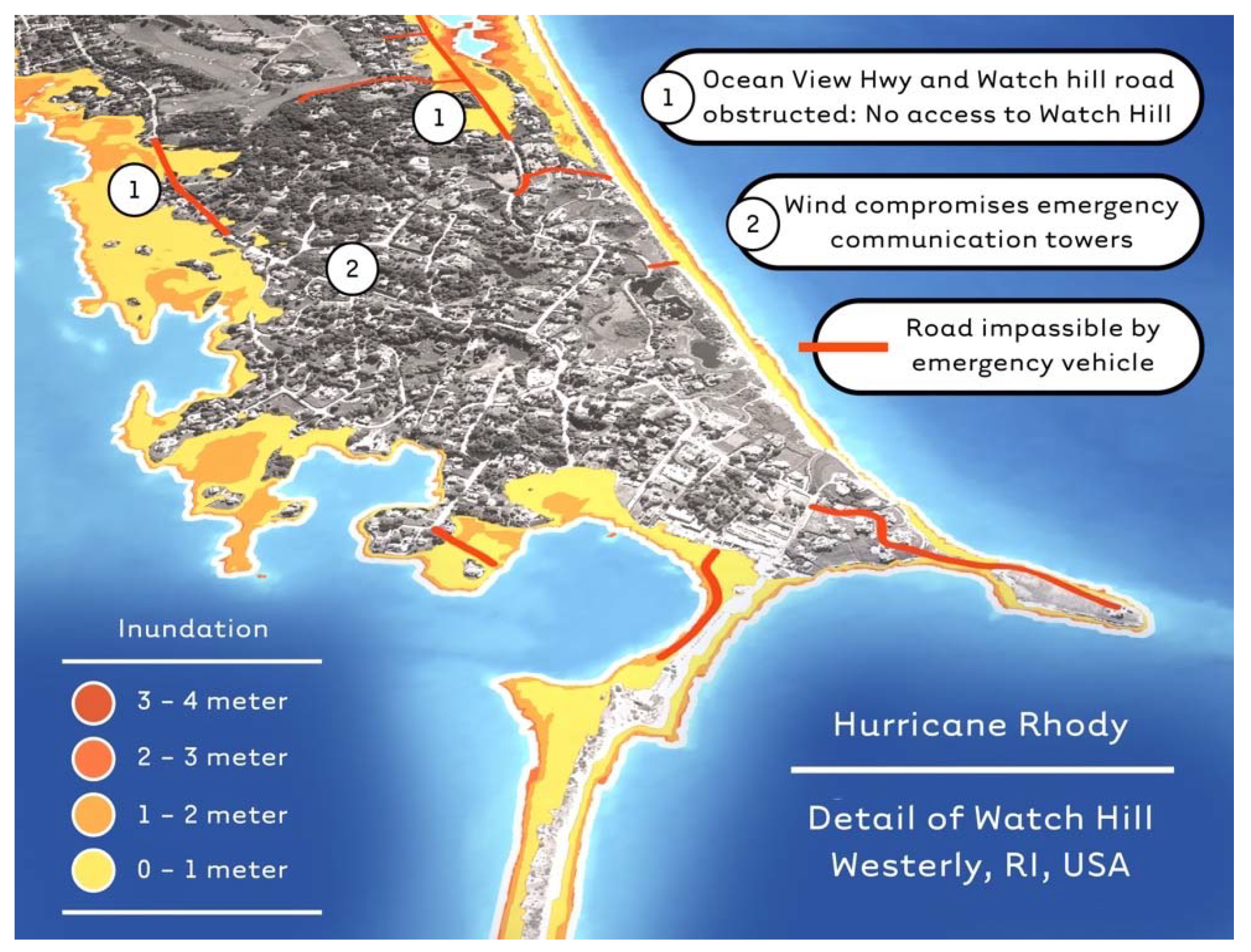
The adaptation of these methods made it possible to extend impact modeling to facilities for which there were not existing damage functions (e.g., communications towers compromised by wind or inundation, or cascading effects of communications outages) (Figure 16). It further provided a credible basis for including areas of concern that are not conventionally captured by point based analysis (e.g., needed evacuation of a trailer park based on ground saturation and wind, creating a treefall hazard).
It also provided an opportunity for local emergency managers and emergency managers overseeing the process to participate in the development of the hazard impact modeling, such that outcomes tested in the models reflected ongoing stakeholder input. This involvement of participants has the potential to increase transparency and make the technical aspects of the process less of a “black box” [17]. This participation may serve to enhance the perceived legitimacy of the outputs and build faith in the process [24]. The further development of these methods thus not only expands the range of impacts that can be credibly modeled at a granular scale, it may be critical to the perceived credibility of the underlying processes [24].

6. Next Steps

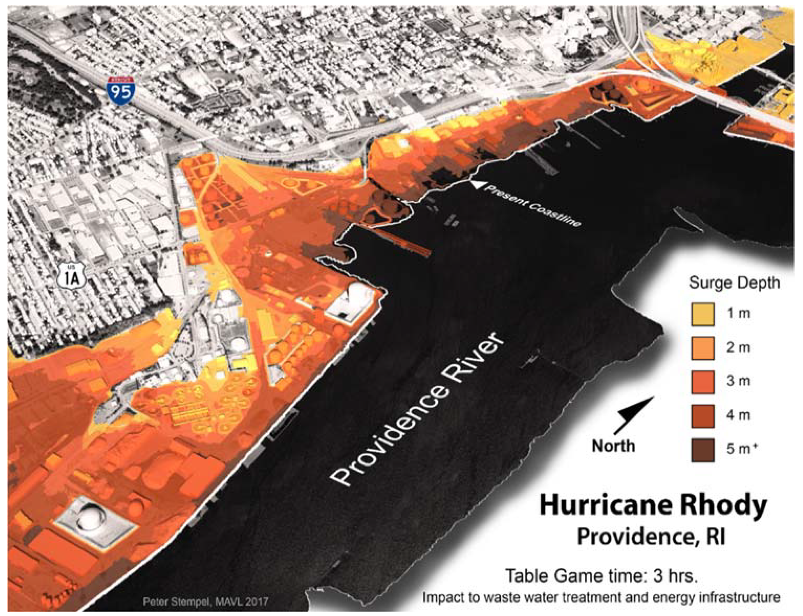
The all numerical method for hazard impact modeling has been developed as part of a larger effort to connect high resolution ocean models to detailed 3D visualizations. This is accomplished by indexing 3D model assets of structures and objects such as buildings, bridges, telephone poles, and debris objects to the previously described geographic points. In the context of the IEMC, the use of these visualizations was confined to depicting inundation (Figure 17) for two reasons:
(1)
While the potential of 3D visualizations to make it difficult to imagine impacts seem more tangible is widely acknowledged [43,44], the effects of such visualizations on perceptions of risk, however, is less clear [22,45]. There are concerns that highly detailed depictions of impacts may make uncertain outcomes appear more certain than they are by virtue of contextualizing less detailed information in highly specific contexts [22]. Further research is needed to better understand the effects of these visualizations on risk perception. The development of the thresholds database, and the implementation of iterative processes involving end users is based in part on practices that are intended to contextualize and support the use of visualizations [46]. These practices will be further developed and refined based on the outcome of this work.
(2)
At the time of the IEMC, databases had only been developed for a limited number of sites and facilities. Representations that mix structures for which there is highly detailed information available with structures for which there is no data may create misleading impressions due to the absence of reported effects. To the extent that specific vulnerability information is gathered from multiple emergency managers, there is also a concern regarding the consistency of the reported data for modeling purposes. This requires further development of consistent methodologies to elicit vulnerability data. The implementation of the databases as part of the IEMC has led to an ongoing collaboration between RIEMA and URI to develop more comprehensive databases for critical facilities in the state.

7. Conclusions

This work integrated advanced hydrodynamic modeling using ADCIRC and SWAN with purpose made geographic information using an all numerical method. Geographic databases were verified against real conditions and were developed in close collaboration with RIEMA and local facility managers to ensure suitability. The implementation of these methods as part of the IEMC suggested that there was merit in the use of time incremented impact analysis to better understand the progression of storm impacts. For instance, impacts of the 1938 Long Island Express Hurricane that is often referenced by citizens and emergency managers in Rhode Island unfolded with particular swiftness for much of the state [47,48]. The simulated storm used for the IEMC, by contrast, combined rapid storm surges and lingering rain and wind effects over multiple days. The effects of the volume of rainfall generated by the storm was more similar to Hurricane Harvey, which made landfall two months after the exercise, than it was to the Long Island Express [47,49]. The catastrophic effects of rainfall of Hurricane Harvey are a stark reminder that hurricanes may do damage through means that are not anticipated by the public or emergency managers [49], and that may be very different from previously experienced storms. This may be especially important at a time when, through the use of high-resolution modeling, we can anticipate the possibility of highly unlikely but catastrophic events [50].
The use of time incremented hazard impact modeling also raises questions regarding the compression of events in training exercises. Damage modeling provided by the Department of Homeland Security Office of Cyber and Infrastructure Analysis that was also used in the exercise indicated wind caused power outage for 80–100% of the state 24 h before the first storm surge made landfall. This placed substantial impacts prior to the bulk of the exercise, which was centered on the first of two storm surges. Furthermore, maximum rainfall occurred in the days following the first surge, prior to a second lesser surge making landfall. This points to what may be a larger issue to be aware of during training: the compression and the potential mis-ordering of anticipated effects. To the extent that storm impacts can vary widely, chronological impact assessment may be a valuable tool to better anticipate and train for the impacts of hurricanes. These experiences, although limited in scope, suggest that further development of these methods is warranted to improve the capacity to predict and depict the impacts of modeled storms.

Author Contributions

Conceptualization, P.S.; Formal analysis, P.S., I.G. and D.U.; Funding acquisition, I.G. and A.B.; Investigation, P.S., A.B. and R.W.; Visualization, P.S.; Writing–original draft, P.S.; Writing–review & editing, P.S., I.G., D.U. and A.B.

Funding

This work has been supported by Rhode Island Sea Grant; The Coastal Institute-University of Rhode Island; the USDA National Institute of Food and Agriculture, Hatch project 1014166; and by the U.S. Department of Homeland Security under Grant Award Number 2015-ST-061-ND0001-01. The views and conclusions contained in this document are those of the authors and should not be interpreted as necessarily representing the official policies, either expressed or implied, of the U.S Department of Homeland Security.

Acknowledgments

Peter Stempel was previously affiliated with the University of Rhode Island, Department of Marine Affairs (2014–2018) where significant portions of this work were conducted. This work would not have been possible without the cooperation of the Rhode Island Emergency Management Agency, The Federal Emergency Management Agency Emergency Management Institute, and the Department of Homeland Security Office of Cyber and Infrastructure Analysis. Thank you to Megan Layman for assistance with compiling GIS point data in preparation for sensitivity tests.

Conflicts of Interest

The authors declare no conflict of interest. The funders had no role in the design of the study; in the collection, analyses, or interpretation of data; in the writing of the manuscript, or in the decision to publish the results.

References

  1. Haraguchi, M.; Kim, S. Critical infrastructure interdependence in New York City during Hurricane Sandy. Int. J. Disaster Resil. Built Environ. 2016, 7, 133–143. [Google Scholar] [CrossRef]
  2. Brecht, H. Geo-technologies in hurricane research. Cartogr. Geogr. Inf. Sci. 2007, 34, 153–154. [Google Scholar] [CrossRef]
  3. Ginis, I.; Kincaid, C.; Hara, T.; Rothstein, L.; Ullman, D.S.; Huang, W.; Rosa, K.; Chen, X.; Zhou, X.; Rubinoff, P.; et al. Modeling the Combined Coastal and Inland Hazards from High-Impact Hypothetical Hurricanes. Appendix to the Annual Project Performance Report Prepared for the DHS Coastal Resilience Center; University of Rhode Island: South Kingstown, RI, USA, 2017. [Google Scholar]
  4. Aerts, J.C.J.H.; Botzen, W.J.; Clarke, K.C.; Cutter, S.L.; Hall, J.W.; Merz, B.; Michel-Kerjan, E.; Mysiak, J.; Surminski, S.; Kunreuther, H. Integrating human behaviour dynamics into flood disaster risk assessment. Nat. Clim. Chang. 2018, 8, 193–199. [Google Scholar] [CrossRef] [Green Version]
  5. Allen, T.R.; McLeod, G.; Sanchagrin, S. Visualization for Hurricane Storm Surge Risk Awareness and Emergency Communication; INTECH Open Access Publisher: London, UK, 2013. [Google Scholar]
  6. Allen, T.; Sanchagrin, S.; Lee, N. Geovisualization Strategies to Analyze and Communicate Inundation Risk from Storm Surges. In Proceedings of the Coastal Society’s 22nd International Conference, Wilmington, NC, USA, 13–16 June 2010; pp. 1–5. [Google Scholar]
  7. Vickery, P.J.; Skerlj, P.F.; Lin, J.; Twisdale, L.A., Jr.; Young, M.A.; Lavelle, F.M. HAZUS-MH hurricane model methodology. II: Damage and loss estimation. Nat. Hazards Rev. 2006, 7, 94–103. [Google Scholar] [CrossRef]
  8. Kopp, R.E.; Horton, R.M.; Little, C.M.; Mitrovica, J.X.; Oppenheimer, M.; Rasmussen, D.; Strauss, B.H.; Tebaldi, C. Probabilistic 21st and 22nd century sea-level projections at a global network of tide-gauge sites. Earth’s Future 2014, 2, 383–406. [Google Scholar] [CrossRef] [Green Version]
  9. Spaulding, L.M.; Grilli, A.; Damon, C.; Crean, T.; Fugate, G.; Oakley, A.B.; Stempel, P. STORMTOOLS: Coastal Environmental Risk Index (CERI). J. Mar. Sci. Eng. 2016, 4, 54. [Google Scholar] [CrossRef]
  10. Fenech, A.; Chen, A.; Clark, A.; Hedley, N. Building an adaptation tool for visualizing the coastal impacts of climate change on Prince Edward Island, Canada. In Climate Change Adaptation in North America; Springer: Cham, Switzerland, 2017; pp. 225–238. [Google Scholar] [CrossRef]
  11. Sneath, S. Predicting flood locations, depths, is aim of new computer simulation. In NOLA.com | The Times Picayune; NOLA Media Group: New Orleans, LA, USA, 2017. [Google Scholar]
  12. Becker, A. Using boundary objects to stimulate transformational thinking: storm resilience for the Port of Providence, Rhode Island (USA). Sustain. Sci. 2017, 12, 477–501. [Google Scholar] [CrossRef]
  13. Stempel, P.; Becker, A. Data Driven Visualization. In Proceedings of the Estuarine and Coastal Modeling Conference, South Kingstown, RI, USA, 14–15 June 2016. [Google Scholar]
  14. Laniak, G.F.; Olchin, G.; Goodall, J.; Voinov, A.; Hill, M.; Glynn, P.; Whelan, G.; Geller, G.; Quinn, N.; Blind, M. Integrated environmental modeling: a vision and roadmap for the future. Environ. Model. Softw. 2013, 39, 3–23. [Google Scholar] [CrossRef] [Green Version]
  15. Kelly, R.A.; Jakeman, A.J.; Barreteau, O.; Borsuk, M.E.; ElSawah, S.; Hamilton, S.H.; Henriksen, H.J.; Kuikka, S.; Maier, H.R.; Rizzoli, A.E. Selecting among five common modelling approaches for integrated environmental assessment and management. Environ. Model. Softw. 2013, 47, 159–181. [Google Scholar] [CrossRef]
  16. Biljecki, F.; Stoter, J.; Ledoux, H.; Zlatanova, S.; Çöltekin, A. Applications of 3D city models: State of the art review. ISPRS Int. J. Geo-Inf. 2015, 4, 2842–2889. [Google Scholar] [CrossRef] [Green Version]
  17. Schroth, O.; Pond, E.; Sheppard, S.R. Integration of spatial outputs from mathematical models in climate change visioning tools for community-decision making on the landscape scale. In Peer Reviewed Proceedings Digital Landscape Architecture 2011: Teaching & Learning with Digital Methods & Tools, Anhalt University of Applied Sciences; Buhmann, E., Ervin, S., Tomlin, D., Pietsch, M., Eds.; Wichmann: Berlin, Germany, 2011; pp. 246–255. [Google Scholar]
  18. Luettich, R.A., Jr.; Westerink, J.J.; Scheffner, N.W. ADCIRC: An Advanced Three-Dimensional Circulation Model for Shelves, Coasts, and Estuaries. Report 1. Theory and Methodology of ADCIRC-2DDI and ADCIRC-3DL; Coastal Engineering Research Center: Vicksburg, MS, USA, 1992. [Google Scholar]
  19. Sheppard, S.R.; Cizek, P. The ethics of Google Earth: Crossing thresholds from spatial data to landscape visualisation. J. Environ. Manag. 2009, 90, 2102–2117. [Google Scholar] [CrossRef] [PubMed]
  20. Liu, S.B.; Palen, L. The new cartographers: Crisis map mashups and the emergence of neogeographic practice. Cartogr. Geogr. Inf. Sci. 2010, 37, 69–90. [Google Scholar] [CrossRef]
  21. Couclelis, H. The certainty of uncertainty: GIS and the limits of geographic knowledge. Trans. GIS 2003, 7, 165–175. [Google Scholar] [CrossRef]
  22. Kostelnick, J.C.; McDermott, D.; Rowley, R.J.; Bunnyfield, N. A cartographic framework for visualizing risk. Cartogr. Int. J. Geogr. Inf. Geovis. 2013, 48, 200–224. [Google Scholar] [CrossRef]
  23. Gesch, D.B. Analysis of lidar elevation data for improved identification and delineation of lands vulnerable to sea-level rise. J. Coast. Res. 2009, 49–58. [Google Scholar] [CrossRef]
  24. White, D.D.; Wutich, A.; Larson, K.L.; Gober, P.; Lant, T.; Senneville, C. Credibility, salience, and legitimacy of boundary objects: water managers’ assessment of a simulation model in an immersive decision theater. Sci. Public Policy 2010, 37, 219–232. [Google Scholar] [CrossRef]
  25. Gao, K.; Ginis, I. On the equilibrium-state roll vortices and their effects in the hurricane boundary layer. J. Atmos. Sci. 2016, 73, 1205–1222. [Google Scholar] [CrossRef]
  26. Gao, K.; Ginis, I. On the Characteristics of Linear-Phase Roll Vortices under a Moving Hurricane Boundary Layer. J. Atmos. Sci. 2018, 75, 2589–2598. [Google Scholar] [CrossRef]
  27. Booij, N.; Ris, R.C.; Holthuijsen, L.H. A third-generation wave model for coastal regions: 1. Model description and validation. J. Geophys. Res. Oceans 1999, 104, 7649–7666. [Google Scholar] [CrossRef] [Green Version]
  28. Dietrich, J.C.; Zijlema, M.; Westerink, J.J.; Holthuijsen, L.H.; Dawson, C.; Luettich, R.A.; Jensen, R.E.; Smith, J.M.; Stelling, G.S.; Stone, G.W. Modeling hurricane waves and storm surge using integrally-coupled, scalable computations. Coast. Eng. 2011, 58, 45–65. [Google Scholar] [CrossRef]
  29. Coulbourne, B.; Headen, F.L.; Jones, C.; Kennedy, A.; Pagano, M.; Ramanathan, K.; Rogers, S.; Soucy, J.; Young, J. North Atlantic Coast Comprehensive Study: Resilient Adaptation to Increasing Risk; Physical Damage Function Summary Report; United States Army Corps of Engineers: Washington, DC, USA, 2015. [Google Scholar]
  30. Sheppard, S.R.; Shaw, A.; Flanders, D.; Burch, S. Can visualization save the world? Lessons for landscape architects from visualizing local climate change. In Peer Reviewed Proceedings Digital Landscape Architecture 2008: Introduction, Anhalt University of Applied Sciences; Buhmann, E., Heins, M., Pietsch, M., Eds.; Wichmann: Berlin, Germany, 2008; pp. 2–21. [Google Scholar]
  31. Chen, L.; Xu, J.-C. Optimal delaunay triangulations. J. Comput. Math. 2004, 22, 299–308. [Google Scholar]
  32. Padgett, J.; DesRoches, R.; Nielson, B.; Yashinsky, M.; Kwon, O.S.; Burdette, N.; Tavera, E. Bridge damage and repair costs from Hurricane Katrina. J. Bridg. Eng. 2008, 13, 6–14. [Google Scholar] [CrossRef]
  33. Robertson, I.N.; Riggs, H.R.; Yim, S.C.; Young, Y.L. Lessons from Hurricane Katrina storm surge on bridges and buildings. J. Waterw. Port Coast. Ocean Eng. 2007, 133, 463–483. [Google Scholar] [CrossRef]
  34. Chang, J.I.; Lin, C.-C. A study of storage tank accidents. J. Loss Prev. Process Ind. 2006, 19, 51–59. [Google Scholar] [CrossRef]
  35. Lange, E. The limits of realism: perceptions of virtual landscapes. Landsc. Urban Plan. 2001, 54, 163–182. [Google Scholar] [CrossRef]
  36. Schroth, O.; Hayek, U.W.; Lange, E.; Sheppard, S.R.; Schmid, W.A. Multiple-case study of landscape visualizations as a tool in transdisciplinary planning workshops. Landsc. J. 2011, 30, 53–71. [Google Scholar] [CrossRef]
  37. Hayek, U.W.; Halatsch, J.; Kunze, A.; Schmitt, G.; Grêt-Regamy, A. Integrating natural resource indicators into procedural visualisation for sustainable urban green space design. Peer Rev. Proc. Digit. Landsc. Archit. 2010, 361–369. [Google Scholar]
  38. Wynne, B. Sheep farming after Chernobyl: A case study in communicating scientific information. When Science Meets the Public; American Association for Advancement in Science: Washington, DC, USA, 1992; pp. 43–68. [Google Scholar] [CrossRef]
  39. Schneider, P.J.; Schauer, B.A. HAZUS—Its development and its future. Nat. Hazards Rev. 2006, 7, 40–44. [Google Scholar] [CrossRef]
  40. Ranger, N.; Reeder, T.; Lowe, J. Addressing ‘deep’uncertainty over long-term climate in major infrastructure projects: four innovations of the Thames Estuary 2100 Project. EURO J. Decis. Process. 2013, 1, 233–262. [Google Scholar] [CrossRef]
  41. Brown, C.; Werick, W.; Leger, W.; Fay, D. A decision-analytic approach to managing climate risks: Application to the Upper Great Lakes. JAWRA J. Am. Water Resour. Assoc. 2011, 47, 524–534. [Google Scholar] [CrossRef]
  42. Becker, A.; Matson, P.; Fischer, M.; Mastrandrea, M. Towards seaport resilience for climate change adaptation: Stakeholder perceptions of hurricane impacts in Gulfport (MS) and Providence (RI). Prog. Plan. 2014. [Google Scholar] [CrossRef]
  43. Moser, S.C.; Dilling, L. Communicating climate change: closing the science-action gap. In The Oxford Handbook of Climate Change and Society; Oxford University Press: Oxford, UK, 2011; pp. 161–174. [Google Scholar]
  44. Sheppard, S.R. Making climate change visible: A critical role for landscape professionals. Landsc. Urban Plan. 2015, 142, 95–105. [Google Scholar] [CrossRef]
  45. Bostrom, A.; Anselin, L.; Farris, J. Visualizing seismic risk and uncertainty. Ann. N. Y. Acad. Sci. 2008, 1128, 29–40. [Google Scholar] [CrossRef] [PubMed]
  46. Schroth, O. From Information to Participation: Interactive Landscape Visualization as a Tool for Collaborative Planning; vdf Hochschulverlag AG: Zürich, Switzerland, 2010; Volume 6. [Google Scholar]
  47. Allen, E.S. A Wind to Shake the World: The Story of the 1938 Hurricane; Little, Brown: Boston, MA, USA, 1976. [Google Scholar]
  48. Blake, E.S.; Rappaport, E.N.; Jarrell, J.D.; Landsea, C.; Center, T.P. The Deadliest, Costliest, and Most Intense United States Tropical Cyclones from 1851 to 2006 (and Other Frequently Requested Hurricane Facts); NOAA/National Weather Service, National Centers for Environmental Prediction, National Hurricane Center: Miami, FL, USA, 2007.
  49. Pérez-Peña, R.; Chokshi, N.; Fountain, H.; Astor, M.; Turkewitz, J.; Thrush, G.; Hirschfeld-Davis, J. With Death Toll at 30, Storm Makes 2nd Landfall. New York Times, 29 August 2017. [Google Scholar]
  50. Lin, N.; Emanuel, K. Grey swan tropical cyclones. Nat. Clim. Chang. 2016, 6, 106–111. [Google Scholar] [CrossRef]
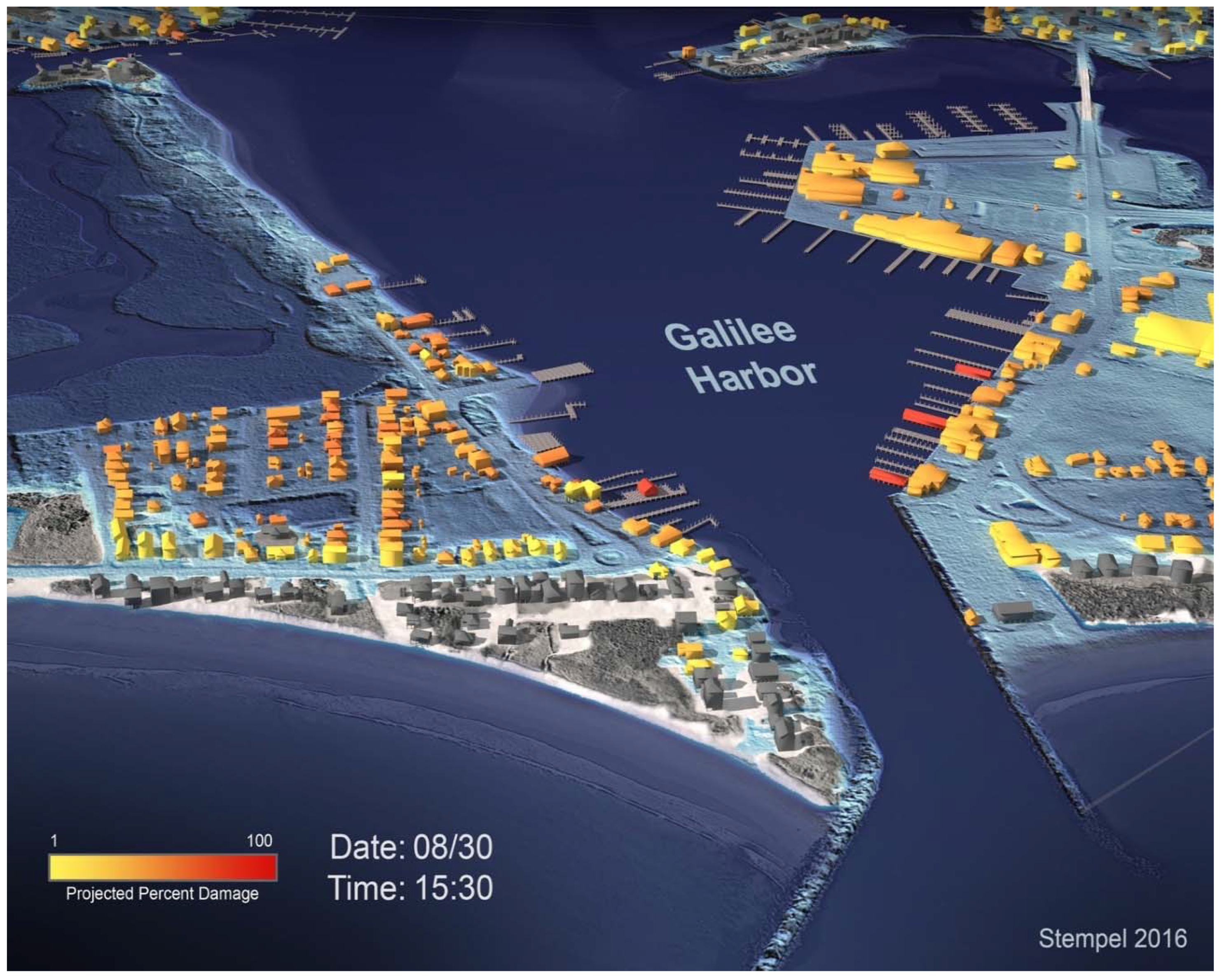
Figure 1. Rendering made during development of the real-time methodology depicting impacts of hurricane Carol (1954) on individual structures in the port of Galilee, RI, USA at current (2016) buildout. Image: Authors.
Jmse 06 00134 g001
Figure 2. Maximum sustained winds (kt) simulated to have occurred during landfall of 1954’s Hurricane Carol, as obtained from the URI HBL model. Image: Authors.
Jmse 06 00134 g002
Figure 3. Hurricane Rhody track. Historical tracks of the 1938 New England Hurricane, Hurricane Carol (1954) and Hurricane Ester (1961) are shown as well. Image: Authors.
Jmse 06 00134 g003
Figure 4. Overview of the hurricane modeling system. Additional modules (e.g., river flooding) may be integrated into this structure. Image: Authors.
Jmse 06 00134 g004
Figure 5. Time series of water level at Providence (top) and Newport (bottom) during Hurricane Carol. Observations are shown in red and model output is denoted by the blue lines. Image: Authors.
Jmse 06 00134 g005
Figure 6. Comparison of conventional workflow and all numeric workflow. Image: Authors.
Jmse 06 00134 g006
Figure 7. Progressive hazard impact model depicting the landfall of hurricane Carol at the port of Galilee, Rhode Island, USA, at present sea level and build out. Hazard impacts for each structure are calculated using the all numerical method and displayed for each timestep (2 shown). Outputs are configured to be directly used by the 3D visualization platform such that damage levels may be displayed for any timestep and updated dynamically. Image: Authors.
Jmse 06 00134 g007
Figure 8. Basic workflow from model(s) to visualization. Output tables may be directly linked to information dashboards or designed to be ingested by visualization platforms such as Unity. Image: Authors.
Jmse 06 00134 g008
Figure 9. Variation in sea surface for nearest adjacent nodes for timesteps during maximum storm surge of Hurricane Rhody in the Fields Point area of the Port of Providence. Where variations are so small, interpolation between nodes may not be necessary. Image: Authors.
Jmse 06 00134 g009
Figure 10. Example of a point with three adjacent nodes (green) and point beyond the nearest wet node (blue). The red lines represent wet portions of the unstructured ADvanced CIRCulation model (ADCIRC) grid. Points tested are both inside and outside of the grid, and constrained by a basin analysis. Image: Authors (Air photo: Rhode Island Geographic Information System (RIGIS)).
Jmse 06 00134 g010
Figure 11. Variation from mean sea surface elevation during a modeled inundation event. Total variation +/− 1 m; total area shown 14 km2. Image: Authors (Air photo: RIGIS).
Jmse 06 00134 g011
Figure 12. Implications of point location. Points used without verifying location in relationship to a vulnerability risk the creation of misleading results. While this may be less of a problem at geographic scales, specific impact assessments require specific data regarding individual vulnerabilities. The concept of “thresholds” is subsequently detailed in this paper. Image: Authors.
Jmse 06 00134 g012
Figure 13. Comparison of points located at highway access ramps and bridge ends (red points) to span centers (green points). Before being corrected, span elevation was recorded as the channel bottom (bathymetry). A more logical way to determine whether a span would be compromised would be to ascertain elevation based on the underside of the span (direct impact/shear failure) or at pier locations (scour) [32,33]. Image: Authors (Air photo: RIGIS).
Jmse 06 00134 g013
Figure 14. Example of micro-topographical condition. The gasometer is protected by an armored concrete dike that is not ‘visible’ to the ocean model. Determining inundation extents without accounting for this dike will lead to misleading results. Image: Authors (Air photo: RIGIS).
Jmse 06 00134 g014
Figure 15. Inundation of downtown Providence by river flooding based on a possible failure of the Fox Point Hurricane Barrier. The realization of this scenario involves multiple uncertainties regarding the performance of infrastructure and human responses. The coloration of the structures reflects flooding at ground level. With adequate facility information, the structures may be separately controlled. This example demonstrates how the capacity to visualize 3D space may exceed the capability of the impact model or our understanding of the underlying uncertainties. Image: Authors.
Jmse 06 00134 g015
Figure 16. A detail of triggered events including analysis of roads for ambulance passage and concerns qualitatively reported by facility and emergency managers. Image: Authors.
Jmse 06 00134 g016
Figure 17. Inundation of waste water treatment and petroleum infrastructure near the height of the first surge of the simulated storm (Hurricane Rhody). Structures depicted in the visualizations are individual 3D models that are linked to hazard impact model output tables. The full capability of the visualization was not utilized due to inconsistent coverage of the data. Note the effects of the protective berms are included. Image: Authors.
Jmse 06 00134 g017
Table 1. Summary of sensitivity test of 14 Waste-water treatment facilities in Rhode Island. “Existing-lowest” refers to the lowest existing point tested minus the lowest elevated vulnerability on site.
RangeExisting-LowestHighest-Existing
Max14.185.420.82
Mean4.542.33−0.92
Median3.341.55−0.73