1. Introduction
For ship propulsion controller development and tuning [
1,
2,
3], or for crew training purposes [
4,
5,
6], it is essential to have reliable simulators that are able to predict in real time the behaviour of all the system components involved (engine, mechanical power transmission, propeller, rudder, hull, etc.). In the last fifteen years, the authors have gained experience in the use of Real Time Hardware in the Loop (RT HIL) simulation for the design of the propulsion control systems of important Italian vessels [
1,
2,
3,
7]. RT HIL simulation consists of an in-test setup where the real hardware controller can exchange data with the ship propulsion models (mainly the engine and propeller) that are simulated in real-time. From a practical point of view, the adoption of this approach required us to face two challenges: running the model in real time mode and interfacing it with the real controller. This was successfully achieved for ship propulsion applications equipped with marine gas turbines [
3].
The main engine is one of the most, if not the most, critical propulsion component to be simulated, requiring good precision and possibly a low computation time. Speed and accuracy are the crucial factors for making a model real-time capable, depending on the technological limits of the current computer processors.
In comparison with a marine gas turbine, a simulation process of a turbocharged diesel engine (the most usual prime mover in marine propulsion systems) presents more difficulties in reproducing chemical and thermodynamic phenomena without significantly increasing the simulation running time.
In the literature, different approaches for marine diesel engine simulation are proposed. To strongly reduce the computation time, the engine behaviour is estimated by performance maps in [
8,
9,
10,
11] or empirical correlations in [
12,
13]. The engine torque or power are determined as a function of a reduced number of input parameters, such as rotational speed and fuel rate, while the engine and relative subsystem (turbocharger) dynamics are taken into account by means of time constants. A little more sophisticated approach is used in [
14,
15,
16], where an ideal dual combustion cycle is considered for in-cylinders phenomena calculations, and simple or more complex performance maps are used for turbocharger compressor and turbine behaviour.
However, the best diesel engine simulation results, in terms of in-cylinders phenomena computation, are obtained by a fully thermodynamic actual cycle simulation approach, where the cylinder thermodynamic processes, including combustion, are calculated as crank angle functions. In these models, a “single-zone” [
17,
18,
19,
20] or a “dual-zone” [
21,
22,
23] combustion scheme is adopted. Further possible approaches involve quasi-dimensional combustion models [
24,
25] or CFD (Computational Fluid Dynamics) analyses [
26], while other specific methodologies can be developed for the engine emissions assessment [
27].
For the turbocharger (TC) system modelling, a thermodynamic approach (based on steady state TC compressor and turbine performance maps, dynamic mass ad energy equations for the manifolds and intercooler simulation) increases the simulation running time very slightly; on the contrary, the same cannot be stated as far as the in-cylinders phenomena assessment. For this engine component, the actual cycle approach requires a complicated step-by-step calculation procedure, based on the crank-angle variation, that strongly increases the computation time.
In this paper, a more simple numerical methodology is proposed for the cylinder performance representation, in order to considerably reduce the running time during the diesel engine transients simulation without affecting the results accuracy in comparison with the actual cycle in-cylinders approach. The basic idea is to replace the traditional thermodynamic equations of the cylinder with appropriate multidimensional numerical maps, in order to simplify the calculation process during the simulation, but still creating a dynamic model for the prediction over time of the main characteristics of the engine. An alternative approach could be represented by the application of an Artificial Neural Network (ANN) [
28,
29] although the training of an ANN, reproducing the engine behaviour over time, requires many samples of engine transients (both in accelerations and deceleration conditions). In this regard, the proposed method, based on numerical tables and physical equations (especially for turbocharger dynamics) can avoid the use of ANN together with its long training procedure. However the article does not want to deal with a certain numerical technique, but it wants to present an alternative structure of a diesel engine model to achieve a faster simulation.
The model has been then used to simulate two twin turbocharged high-speed diesel engines powering a motor yacht equipped with two fixed pitch propellers.
The model validation is based on the comparison with the engine manufacturer steady state data and with the boat acceleration and deceleration manoeuvre simulation results, achieved by an actual cycle “single zone” diesel engine model previously developed by the authors [
23].
As for computation speed, in this paper it will be shown that the running time required by the new simulator is about 1% of the fully thermodynamic one [
23]. This result is essential for the development of a diesel engine real-time simulator, since a fast simulation process can be more easily transformed into a real-time executable application.
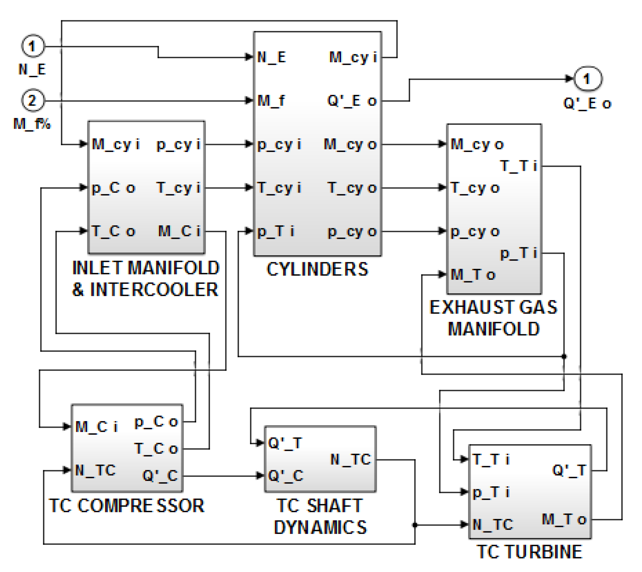
2. Thermodynamic Diesel Engine Simulator
The real-time diesel engine simulator comes from the fully thermodynamic cylinder’s actual cycle model [
23], developed in a Matlab/Simulink environment and consisting of the following modules (
Figure 1):
- -
cylinders;
- -
inlet manifold and intercooler;
- -
exhaust gas manifold;
- -
turbocharger (TC) compressor;
- -
TC turbine;
- -
TC shaft dynamics.
A filling and emptying method is adopted in each simulator module, describing the pertinent subsystem behaviour by means of component performance maps, and algebraic and differential equations. The fluid is modelled as an ideal gas while the specific internal energy and enthalpy are both functions of temperature and fluid composition. A brief description of the engine simulator is reported in the following, however a more detailed explanation can be found in [
23].
2.1. Basic Equations
The fluid is modelled by the ideal gas equation:
where
p is the pressure;
V the volume;
m the fluid mass;
R the gas constant and
T the temperature.
Fluid mass and energy stored in each engine component volume are calculated through the continuity and the energy dynamic equation:
where
ρ is the gas density;
U the gas specific internal energy;
Mi and
Mo the mass flow rate at the inlet and outlet section;
Hi and
Ho the specific enthalpy at the inlet and outlet section;
Mf and
Hf respectively the fuel mass flow rate and lower heating value;
Φ the heat flow and
P the mechanical power.
The turbocharger shaft dynamics equation is:
where
ω is the angular velocity;
J is the total moment of inertia;
Q’T and
Q’C are the turbine and compressor torque, respectively.
2.2. Thermodynamic Cylinder Module
In the thermodynamic module named “cylinders” in
Figure 1, a single zone actual cycle approach is used to assess in-cylinders phenomena. The in-cylinder calculations use the crank angle
θ as an independent variable and start when the inlet valve is open (fresh air charge intake phase) and end at the gas exhaust phase.
The flow through the inlet and exhaust valves is determined by Equation (5) for compressible gas through a flow valve restriction:
In the case of choked flow, the equation used is:
where
pi and
Ti are the pressure and temperature at the inlet section of the cylinder valves;
po is the exhaust manifold pressure;
AR is the valve open area and
k is the ratio of specific heats. The discharging coefficient value
CD is assumed to be equal to 0.7.
The piston displacement from the top dead centre (
x) is determined by the crank angle value through [
30]:
where
r is the crank radius and
l the connecting rod length.
From the x values, it is possible to calculate the in-cylinder volume V of Equations (2) and (3). Using Equation (3), the air compression process is then determined for each crank angle step variation (dθ).
During each calculation step
dθ, the convective gas–cylinder wall heat transfer (
Φ in Equation (3)) is determined as reported in [
31].
The fuel ignition crank angle (
θign) is given by:
where
θinj is the crank angle corresponding to fuel injection starting.
The ignition delay angle
θid, is estimated by the following relationship:
where
Kid is the delay constant;
n is the engine rotational speed;
pcy and
Tcy are the in-cylinder pressure and temperature at the fuel injection beginning; and
CN is the fuel cetane number.
At each calculation step
dθ, the heat
dQf released in the combustion process is determined by:
where
Hf is the fuel lower heating value and
dmb is the fuel mass burned. The latter is obtained through:
with
mf being the total fuel mass injected per cycle. The fuel fraction burned
dxb in Equation (11), during the calculation step
dθ, is determined by the Wiebe equation [
22]:
where
Ka and
Km are numerical constants;
θign is the crank angle corresponding to fuel ignition and Δ
θ is the total combustion angle length.
In each calculation step
dθ, the work done onto the piston (
dW) is calculated by:
where
pc is the in-cylinder pressure during the cycle computation and
dV is the cylinder volume change. The cylinder pressure
pcy is found through the ideal gas equation (Equation 1), once the fluid temperature from the energy equation (Equation 3) is known.
The brake mean effective pressure (
b.m.e.p). is determined by:
where
i.m.e.p is the gross indicate mean effective pressure;
p.m.e.p. is the pumping mean effective pressure and
f.m.e.p. is the mechanical friction mean effective pressure. The latter is evaluated on the basis of test data provided by the engine manufacturer by means of the procedure described in [
15]. Finally, the engine delivered brake torque (
Q’E) can be calculated by:
2.3. Inlet Manifold and Intercooler Module
As shown in
Figure 1, these two components of the engine are simulated through a single module.
The mass and energy accumulation in the considered control volume are determined by means of the pertinent dynamic equations (Equations (2) and (3), respectively).
The air cooling effect is assessed by a heat exchanger efficiency equation. The overall set pressure drop is determined as a function of the inlet pressure and mass flow rate.
2.4. Exhaust Gas Manifold Module
This block, located between the “cylinders” and “TC turbine” modules of the engine simulator of
Figure 1, works in a very similar mode to the intercooler and air receiver modules, by using the dynamic continuity equation (Equation (2)) and the energy equation (Equation (3)). The exhaust manifold temperature
Tex (i.e., the TC turbine inlet gas temperature
T_Ti in
Figure 1) is calculated considering the blow-down effect through the exhaust valve [
31], as follows:
where
Ti and
pi are the in-cylinder temperature and pressure during the unloading phase and
po is the exhaust gas manifold pressure.
2.5. Turbocharger Compressor and Turbine Modules
The compressor behaviour is simulated by a numerical table extrapolated from the manufacturer’s datasheet. It reports the pressure ratio and isentropic efficiency values, both depending on the corrected volume flow rate (
V’Cc) and the corrected rotational speed (
nCc):
where
V’C is the volumetric flow rate;
Ta and
Tref are the ambient and reference temperature respectively and
nTC is the TC rotational speed.
From the compressor pressure ratio and efficiency, it is possible to assess the outlet air pressure and adsorbed torque.
The turbine simulation approach is very similar to the compressor one, since the turbine gas flow rate and efficiency (needed for the delivered torque computation) are estimated by a steady state map depending on the pressure expansion ratio and the kinematic ratio (i.e., the ratio between the rotor speed and the isentropic expansion velocity).
2.6. Turbocharger Shaft Module
The basic Equation (4) is used to calculate the TC shaft angular speed (
N_TC) in the “TC shaft dynamics” engine simulator module in
Figure 1.
2.7. Overall Engine Simulator Input–Output Variables
With reference to
Figure 1, the input variables needed by the engine simulator are the engine speed (
N_E) and the fuel mass flow rate in percentage (
M_f %), referred to as the maximum continuous rating fuel flow consumption. The main simulation output of the engine model is the shaft torque (
Q’_E o).
3. Simplified Cylinder Model
The “cylinders” module of the thermodynamic simulator (
Figure 1) is mainly responsible for the long running time. To speed up the computation time, it was decided to substitute the actual cycle calculation procedure with a simpler methodology. In the new approach, the output results of the “cylinders” module are estimated by five five-dimensional (5-D) matrices, one for each of the following output data:
- (1)
cylinder inlet air flow rate;
- (2)
engine delivered torque;
- (3)
outlet exhaust gas flow rate;
- (4)
outlet exhaust gas temperature;
- (5)
outlet exhaust gas pressure
Figure 2 shows the five input values of a single 5-D table for a faster computation of one of the five considered output data.
In the whole new “cylinders” module, each table evaluates a sampled representation of a function in five variables: inputs are mapped to an output value by looking up or interpolating a table of numerical values, defined in the 5-D matrix.
The input values of every 5-D table are obviously the same as the thermodynamic “cylinders” module of
Figure 1, i.e.: engine speed (
N_E), percent fuel mass flow (
M_f %), cylinder inlet pressure (
p_cy i), temperature (
T_cy i), and exhaust gas outlet pressure (
p_Ti).
The data reported in each of the 5-D matrices are evaluated by running the engine simulator, in the “cylinders” actual cycle configuration, for a large range of engine revolutions. In particular, in order to cover the entire engine working area, the engine speed N_E is considered in a range between 45% and 110% of the engine design value (considering 5% as an incremental step), while the fuel mass flow rate M_f % is tested in the range of 10–110% (10% as an incremental step).
4. Engine Models Application and Validation
The described thermodynamic model (characterised by the actual cycle “cylinders” module [
31]) was recently applied to the performance simulation of two marine engines by Rolls Royce: the diesel engine RR C25:33L6P and the natural gas fed engine RR C26:33L8PG (where in the latter, the “cylinders” module is adapted for the natural gas combustion simulation [
32]). These two engines are characterized by a maximum continuous rating (MCR) power of 2 MW and 2.16 MW respectively, at the same rotational speed (1000 rpm). The comparison between reference and simulation data, reported in [
32], showed a good simulator accuracy: the errors are generally less than 2% in the MCR engine load conditions, and less than 5% in the other examined working conditions of the engines.
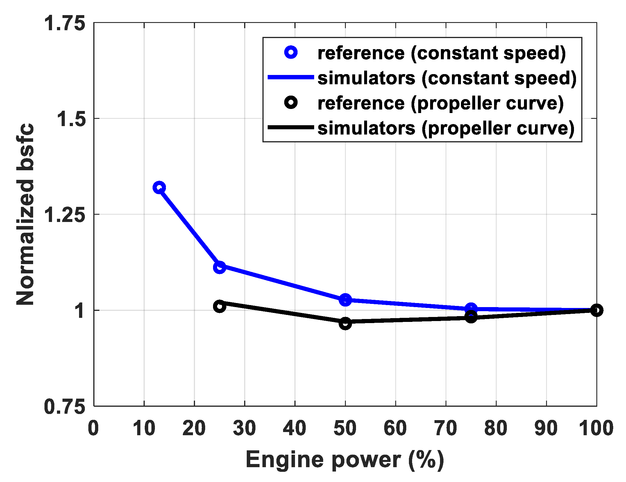
The two engine models described in this paper (i.e., cylinder actual cycle and simplified one) are applied to the simulation of the General Electric (GE) marine 12V 228 four stroke diesel engine, whose main characteristics are reported in
Table 1. The comparison between brake specific fuel consumption (bsfc) reference data and simulation results is reported in
Figure 3. In particular, engine working conditions at propeller and maximum continuous speeds are considered. The simulation accuracy between the actual cycle cylinders module and the 5-D matrices approach is so good that the results appear coincident.
For the sake of completeness, the actual cycle approach was validated in a different application [
22] by comparing simulation results and experimental data about: gross indicated mean effective pressure, the in-cylinder pressure, cylinder wall temperature and heat release rate. The comparison was carried out for three different engine working conditions (brake mean effective pressure equal to 100%, 75% and 50% of MCR) at the rated speed. Only for the cylinder heat release rate, the error between simulation and test data exceeds 1.5% but is still less than 3.5% (further details can be found in [
22]). Unfortunately, for the engine considered in the present work, only brake specific fuel consumption data are available for the simulation validation process.
5. Yacht Propulsion Plant Simulator
In order to verify the performance of the above described diesel engine models in transient conditions and to compare the respective simulation accuracy and computation time, both approaches are used in a motor-yacht propulsion simulator again developed in a Matlab/Simulink environment.
Table 2 shows the main ship characteristics, whose propulsion system is equipped with two fixed pitch propellers, each one driven through a gearbox by a GE marine 12V 228 four stroke diesel engine.
The numerical simulation techniques to assess the ship performance were already described and validated in [
33]. However, a brief description of the yacht propulsion plant simulator is repeated hereinafter. The open water propeller data (Wageningen series) have been adopted for the propeller modelling. By equations:
where the propeller thrust
Tp and torque
Q’p are functions of the thrust
Kt and torque
KQ coefficients (both depending on the propeller advance coefficient), the propeller diameter
D and rotational speed
Np;
ρsw is the sea water density.
Once propeller torque is calculated, the propeller speed
Np is determined by the shaft dynamics equation:
where
Jpolar is the total inertia polar moment of the all rotational masses (engine, gearbox and propeller plus added water mass);
Q’E is the main engine brake torque;
Q’p is the open water propeller torque;
ηr is the propeller shaft efficiency and
Q’f represents the gear frictional losses (considered as a percentage of the engine delivered torque).
The gearbox is modelled by the gear ratio, mechanical efficiency and inertia.
Ship dynamics are evaluated in one degree of freedom, taking into account only the hull surge motion. Ship speed
Vs is calculated by solving the differential equation:
where
ms and
mad are the ship mass and added water mass;
z is the number of the working propellers and
Tp the single propeller thrust;
tp is the thrust deduction factor and
Rt the hull total resistance, depending on
Vs.
In this application, the engine throttle valve is controlled by a proportional and integral action of the governor. The bridge lever position requires the propeller speed, that is compared with the effective one. The speed error is then the input data of the engine governor, whose output is the fuel mass flow rate (
M_f % in
Figure 1). The fuel pump and injection system delays are modelled by a time constant.
6. Yacht Manoeuvre Simulation
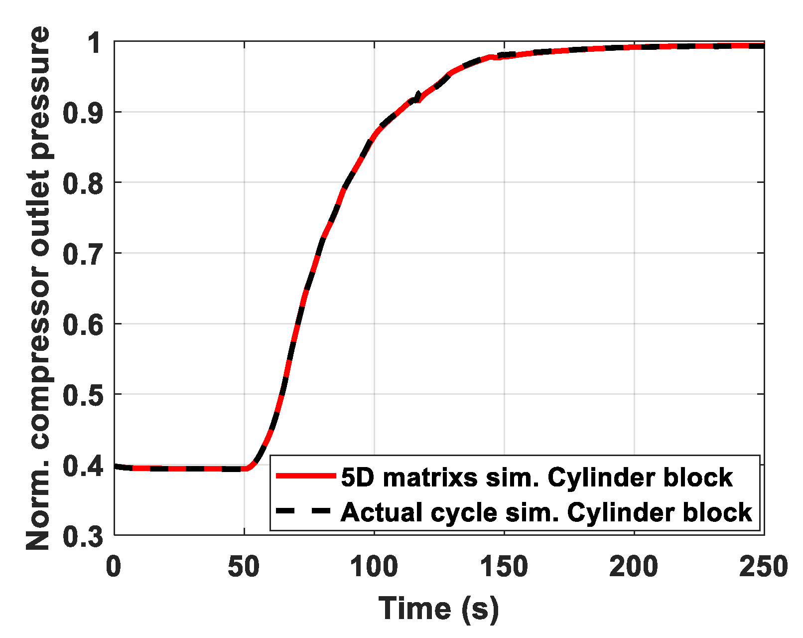
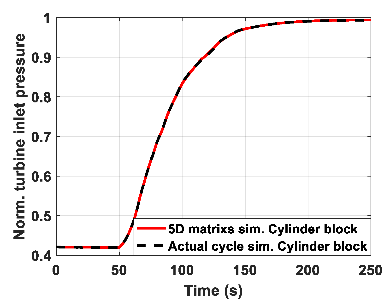
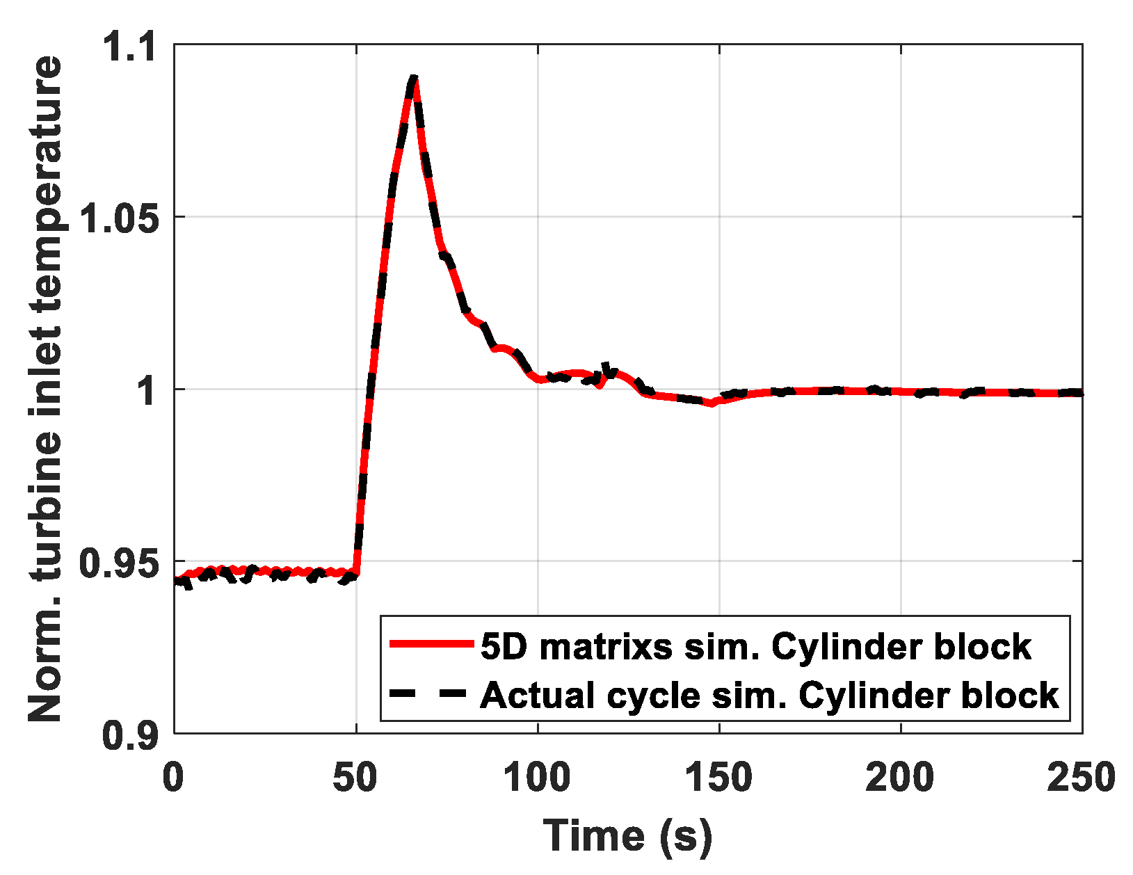
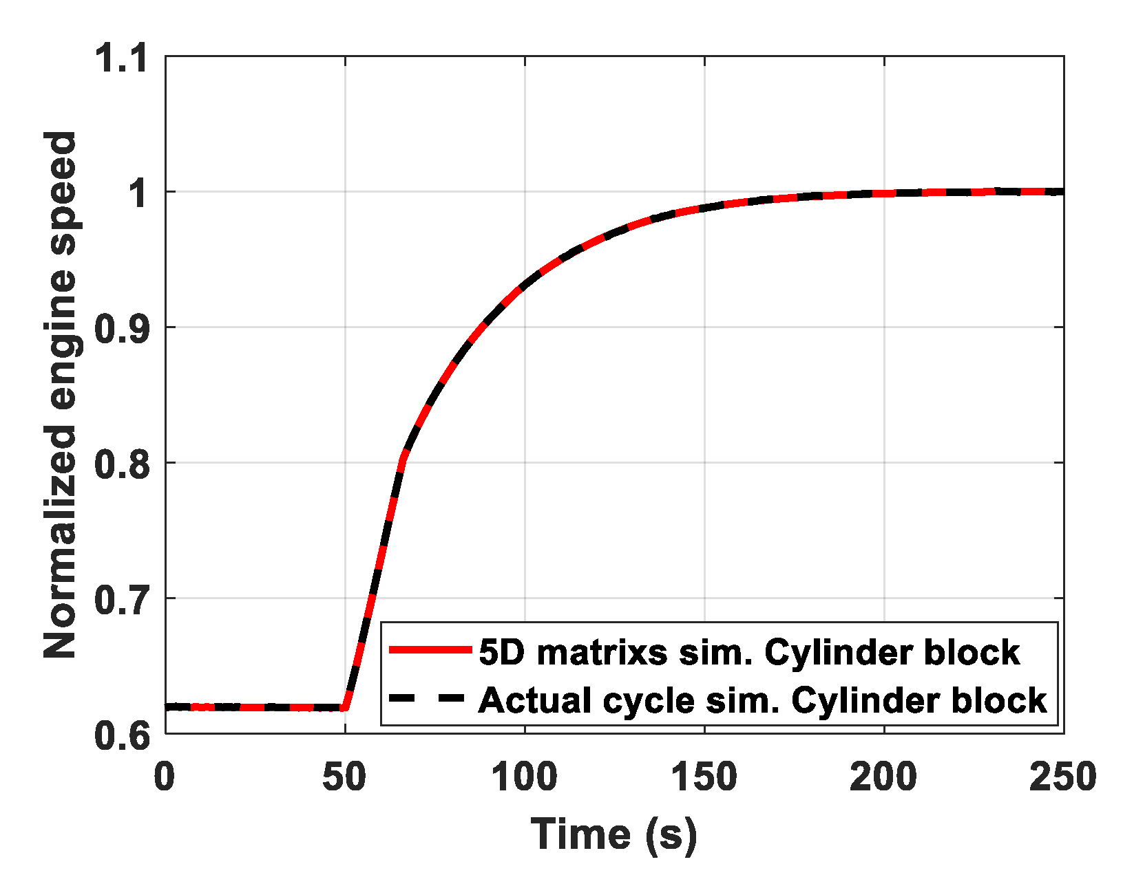
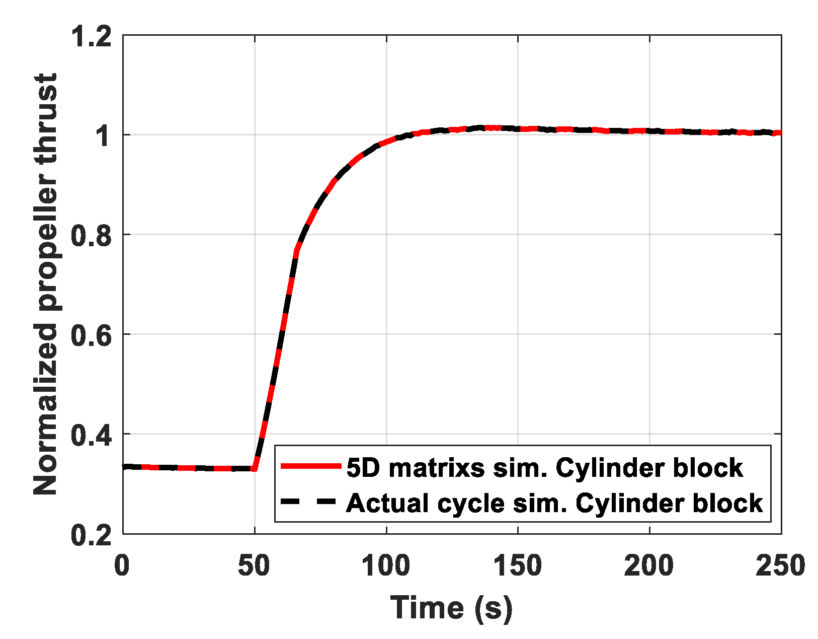
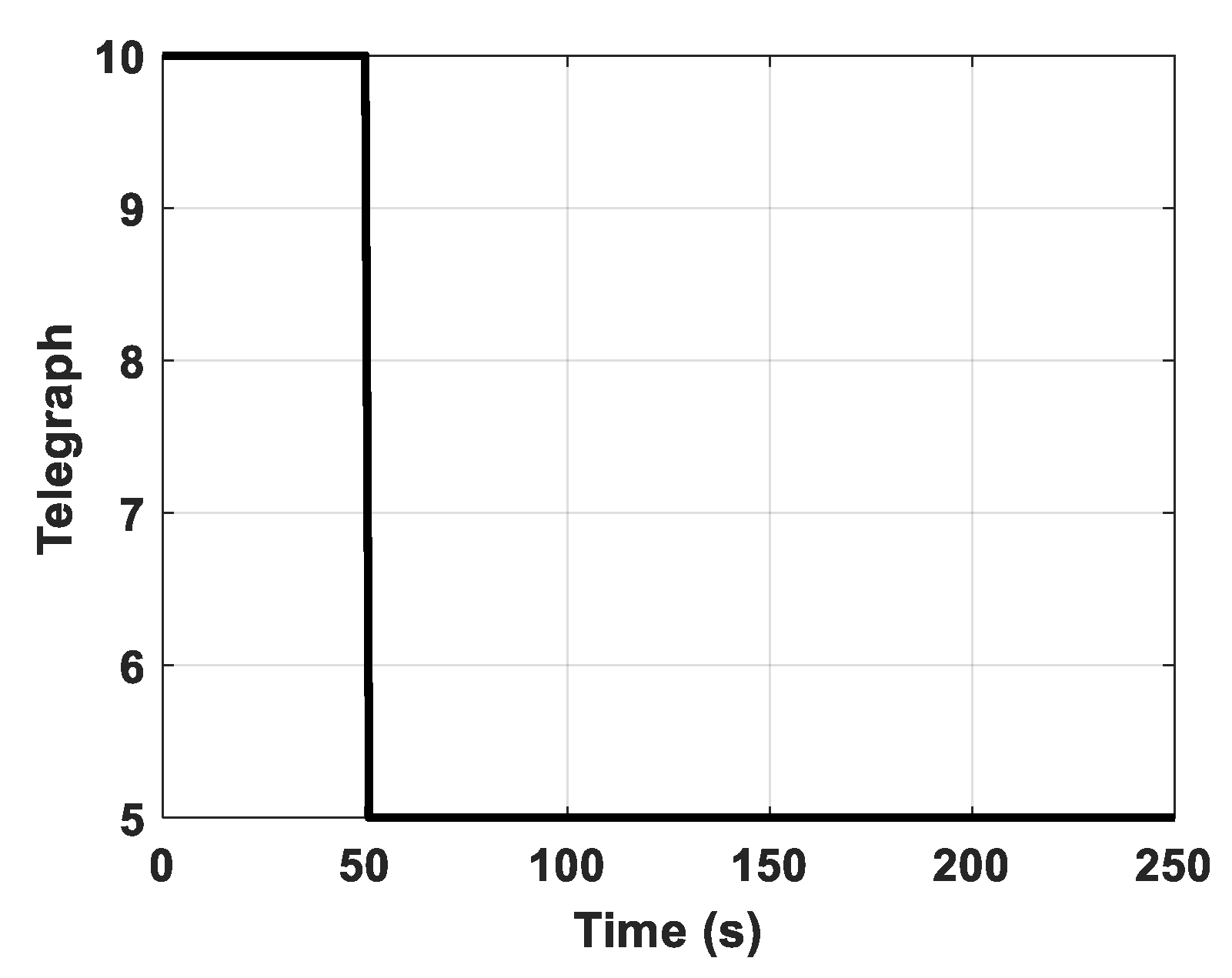
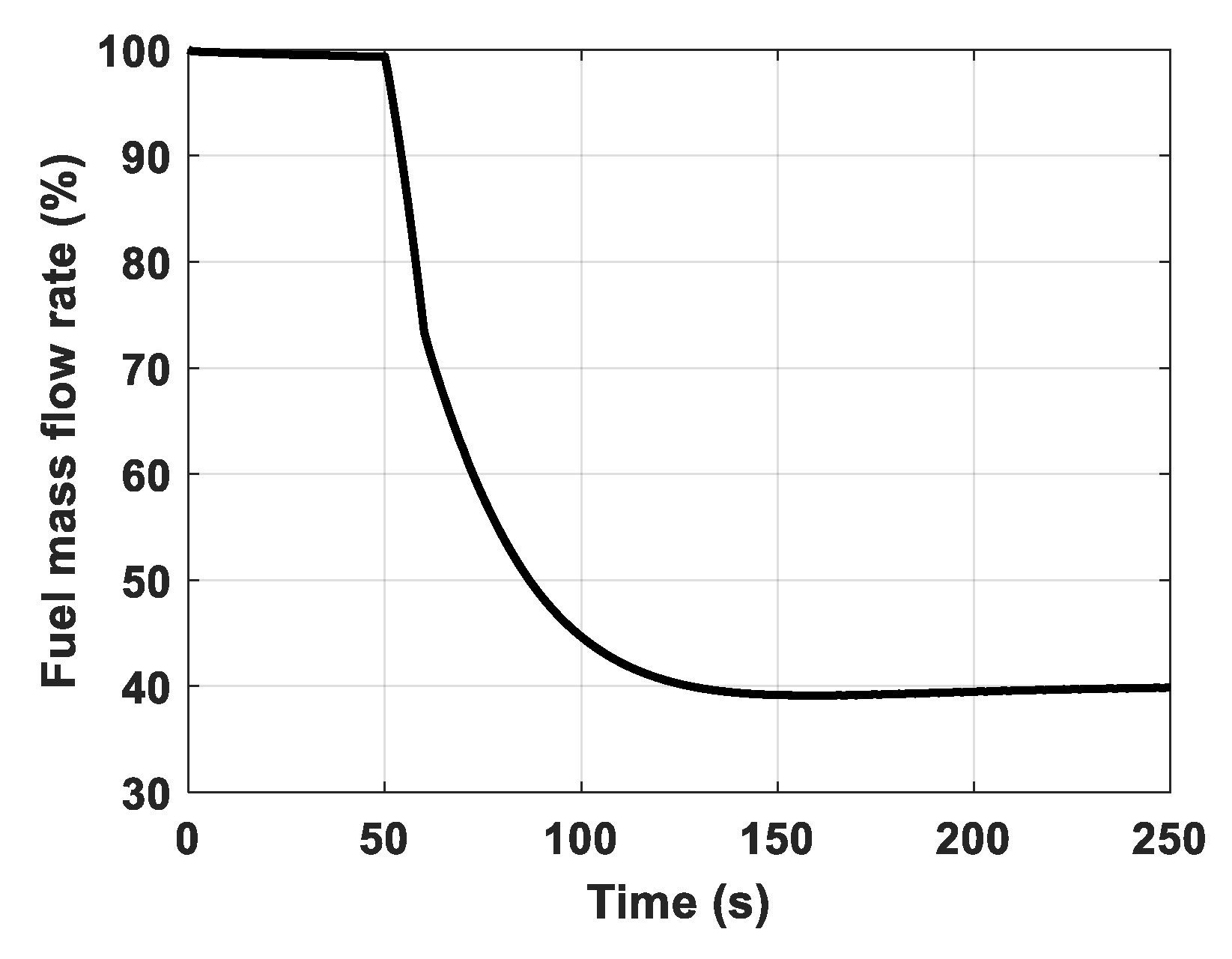
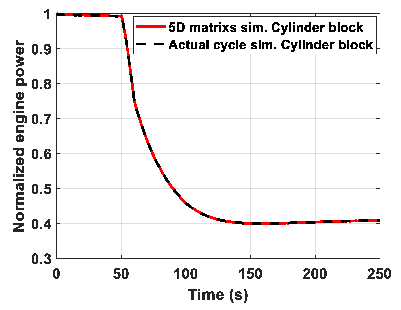
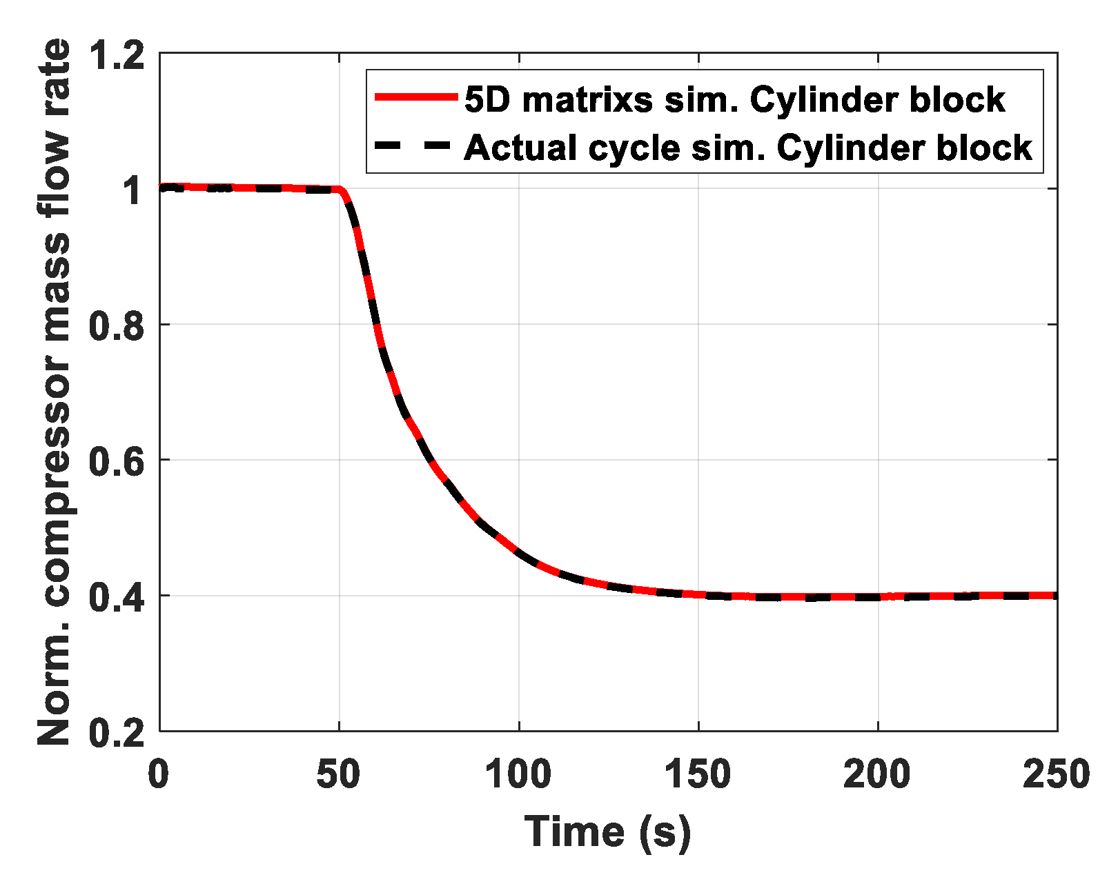
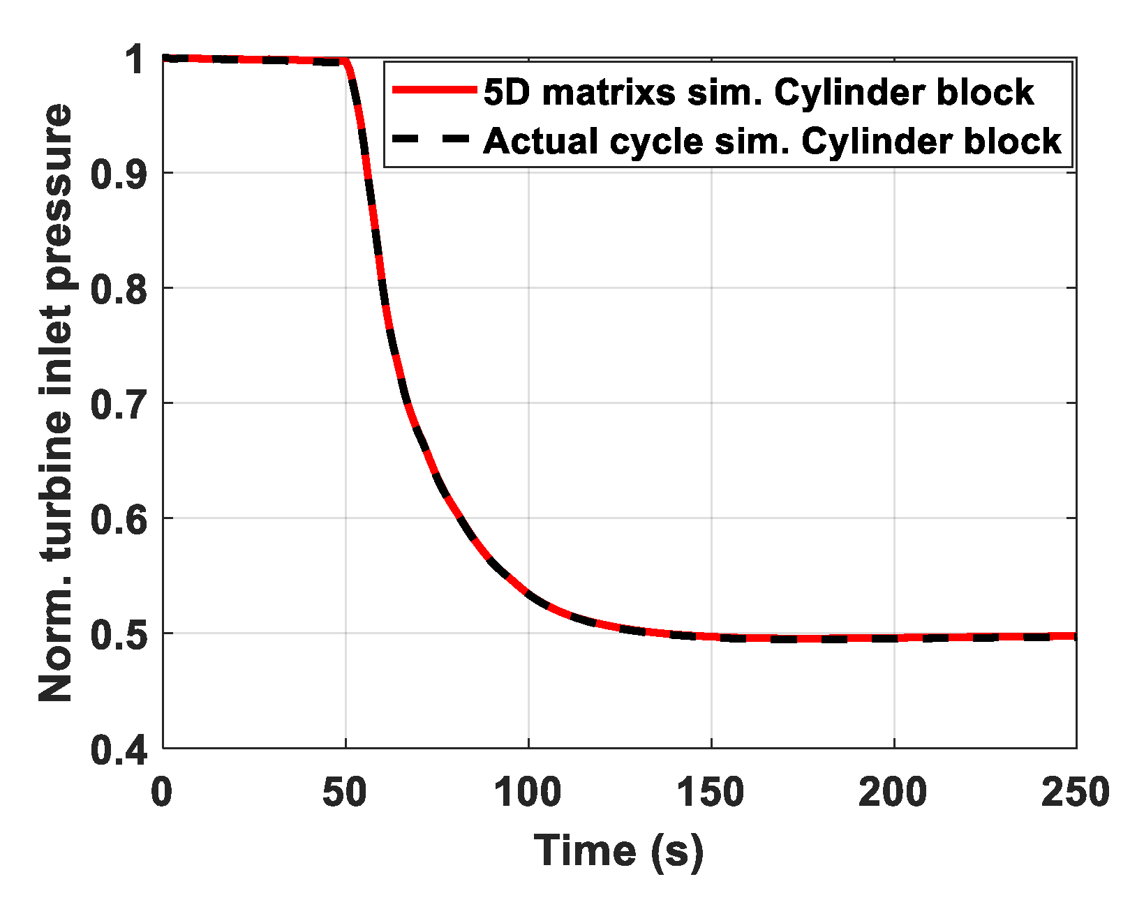
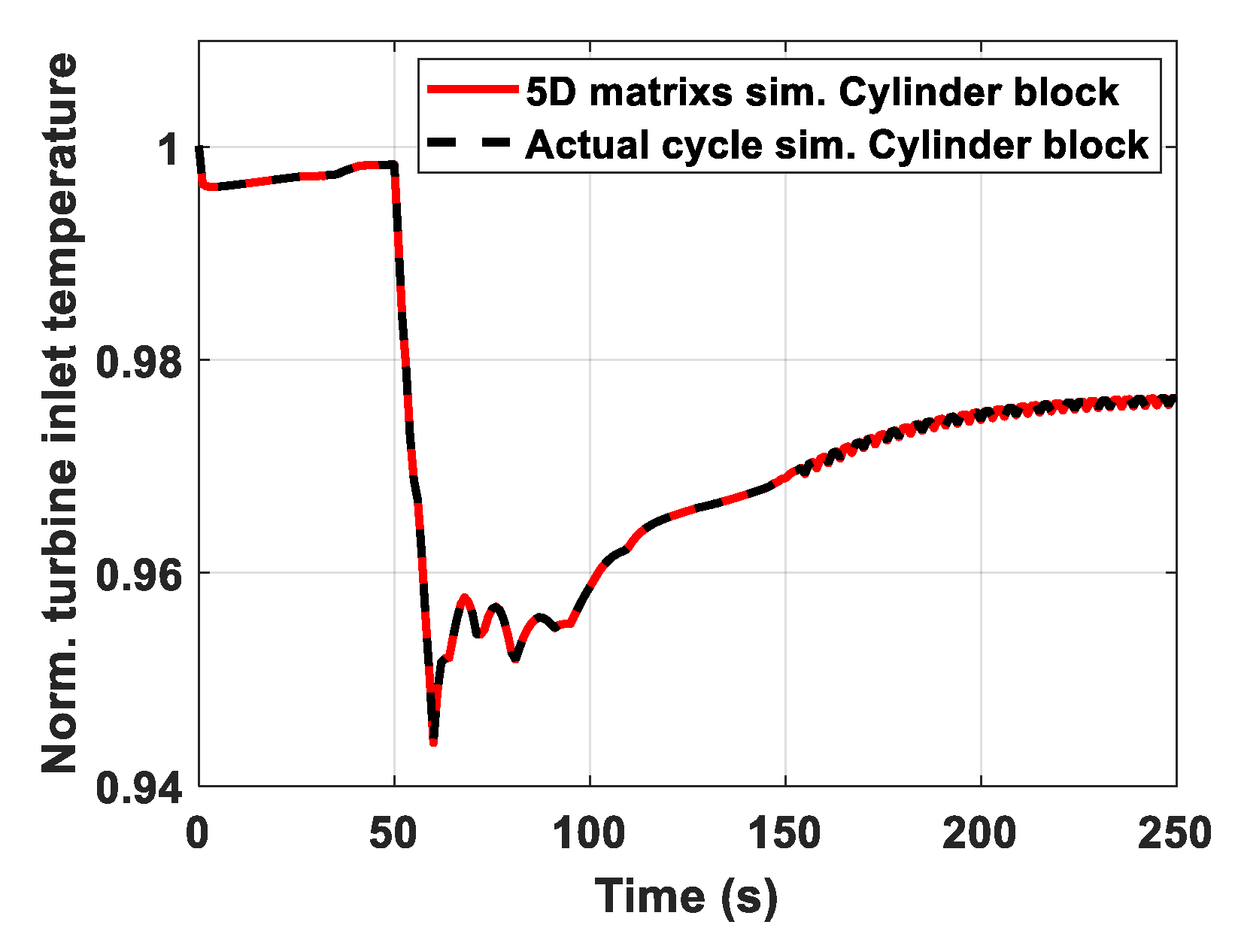
Boat acceleration and deceleration manoeuvres are simulated to compare behaviour and computation time of the actual cycle “cylinders” method with the 5-D matrices approach. Many simulation values reported in the following figures are normalized on the basis of the MCR engine running conditions.
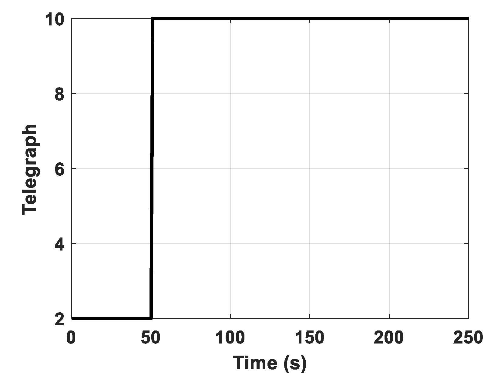
The first transient considered for the engine simulators comparison is yacht acceleration due to the lever step increase from two up to 10, as visualized in
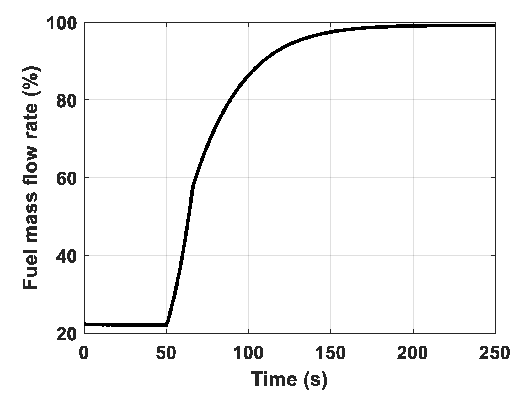
Figure 4. The fuel mass flow rate percentage managed by the engine governor increases over time, as shown in
Figure 5.
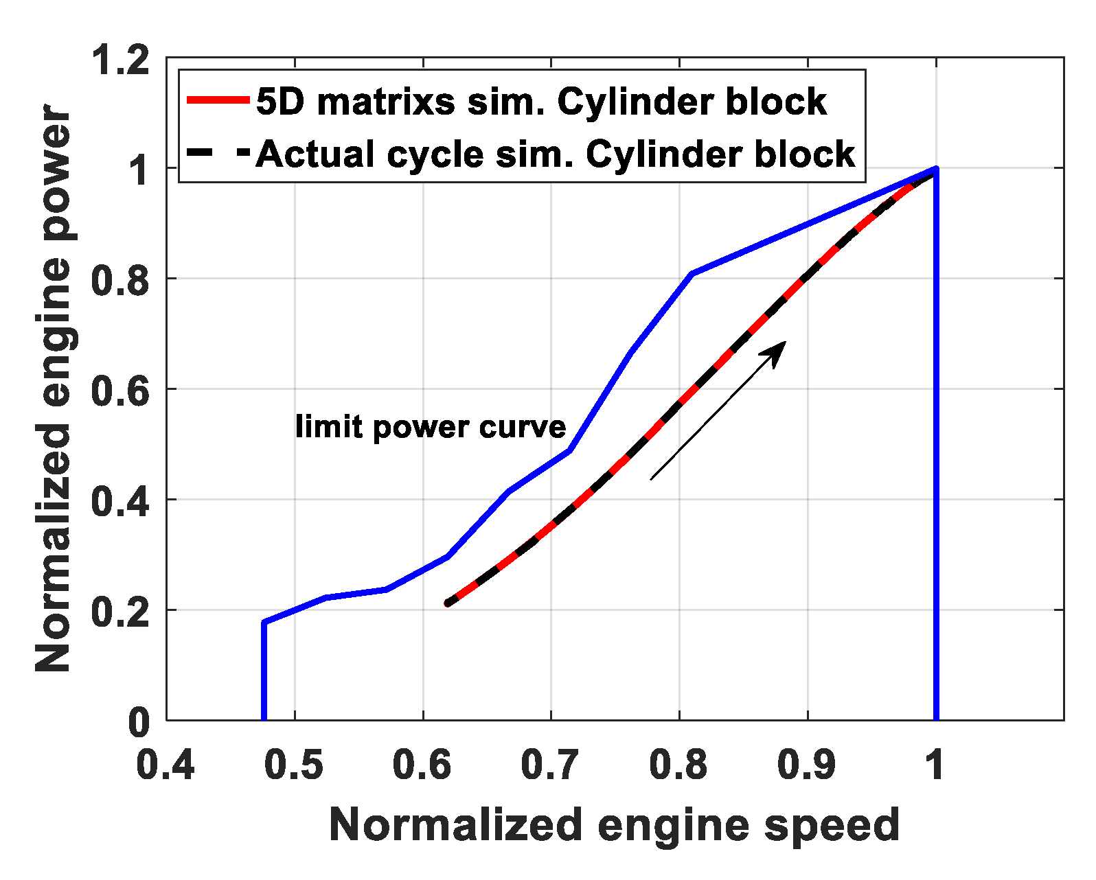
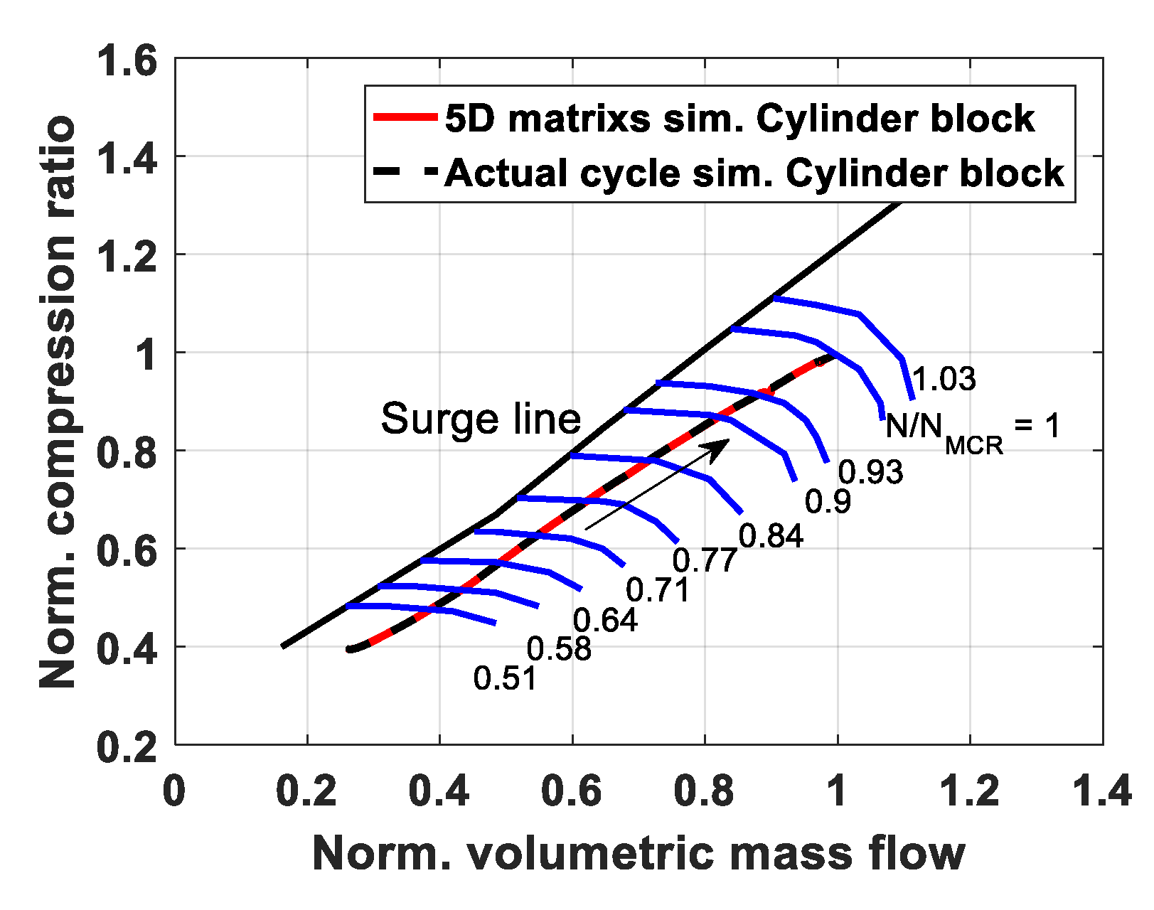
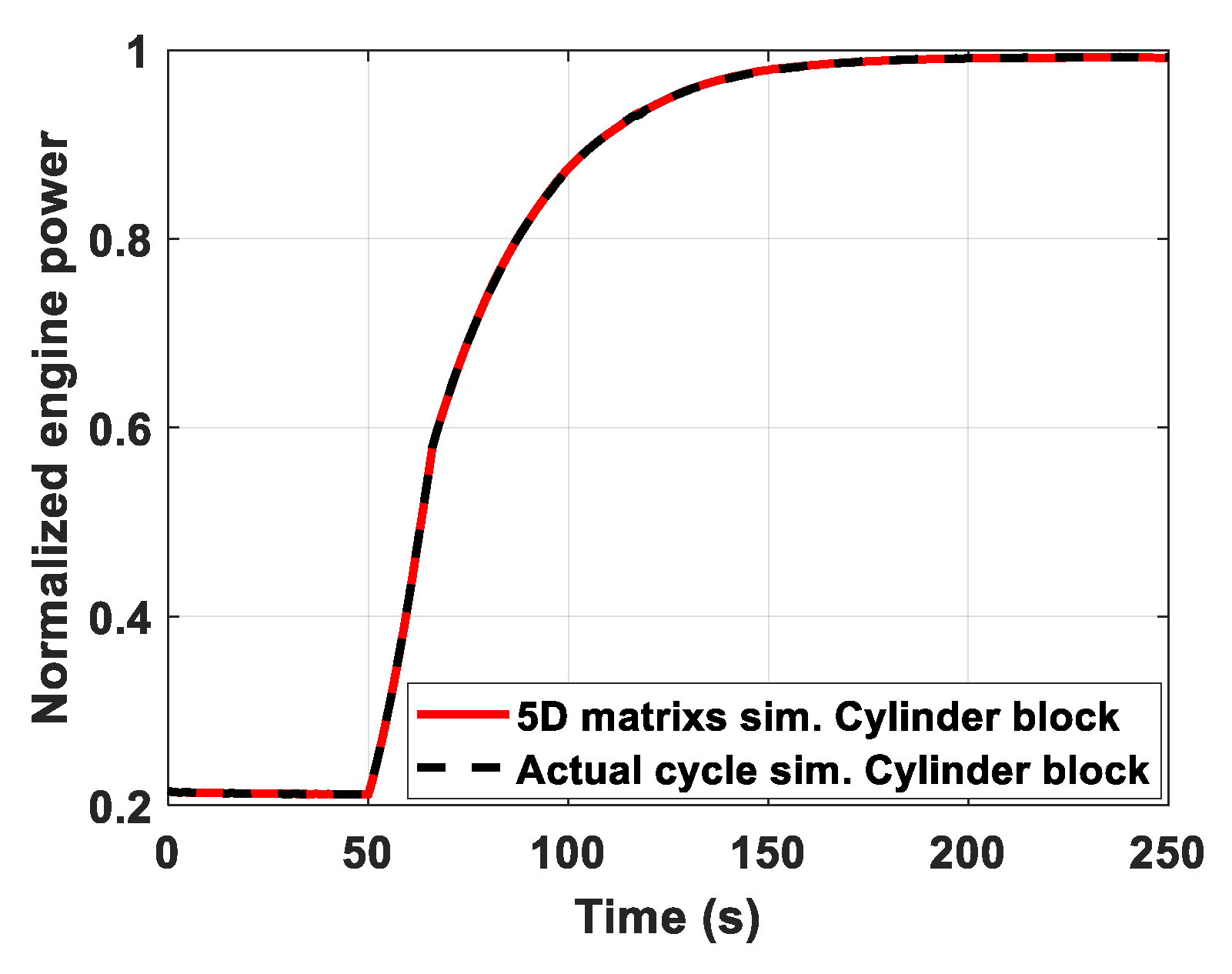
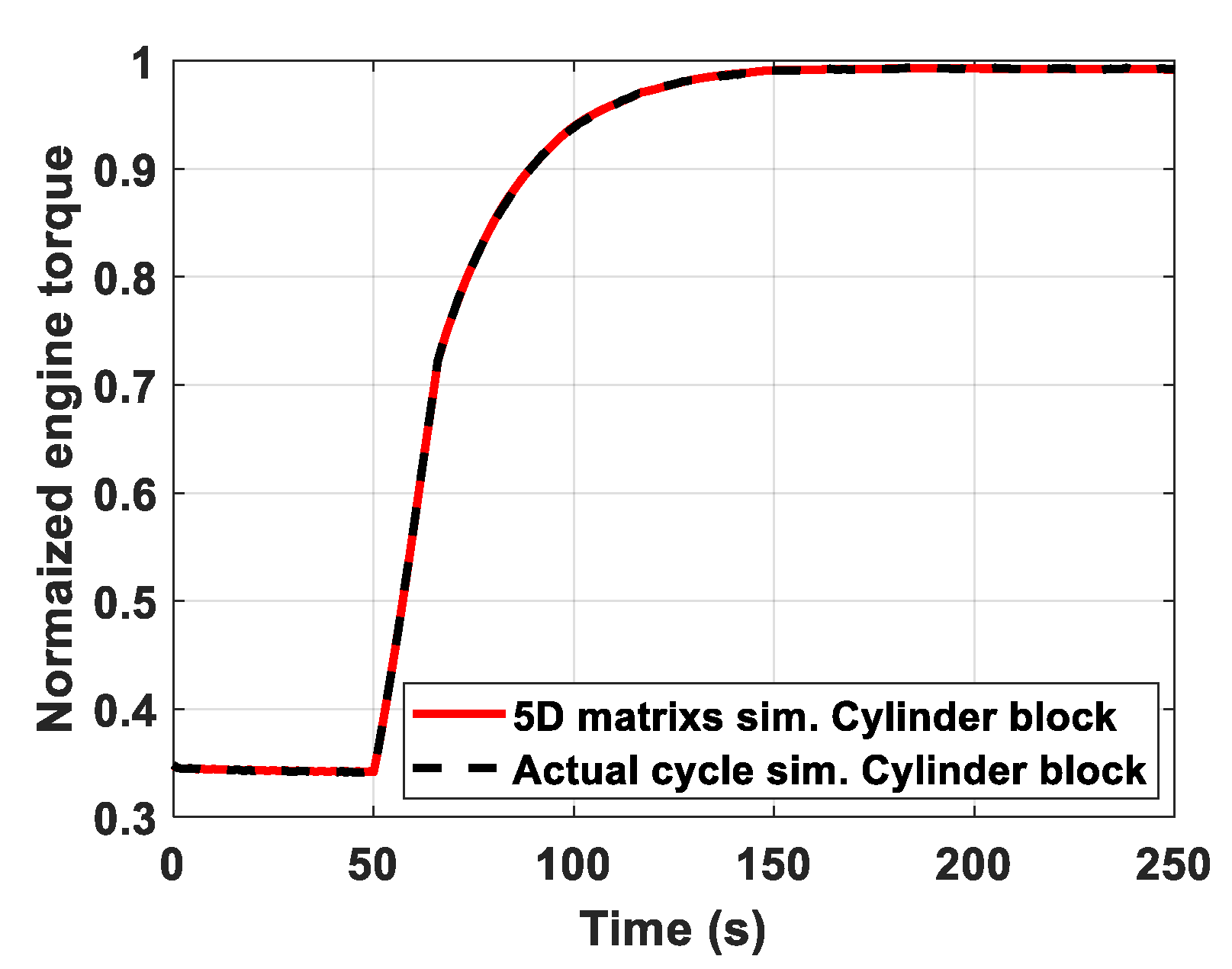
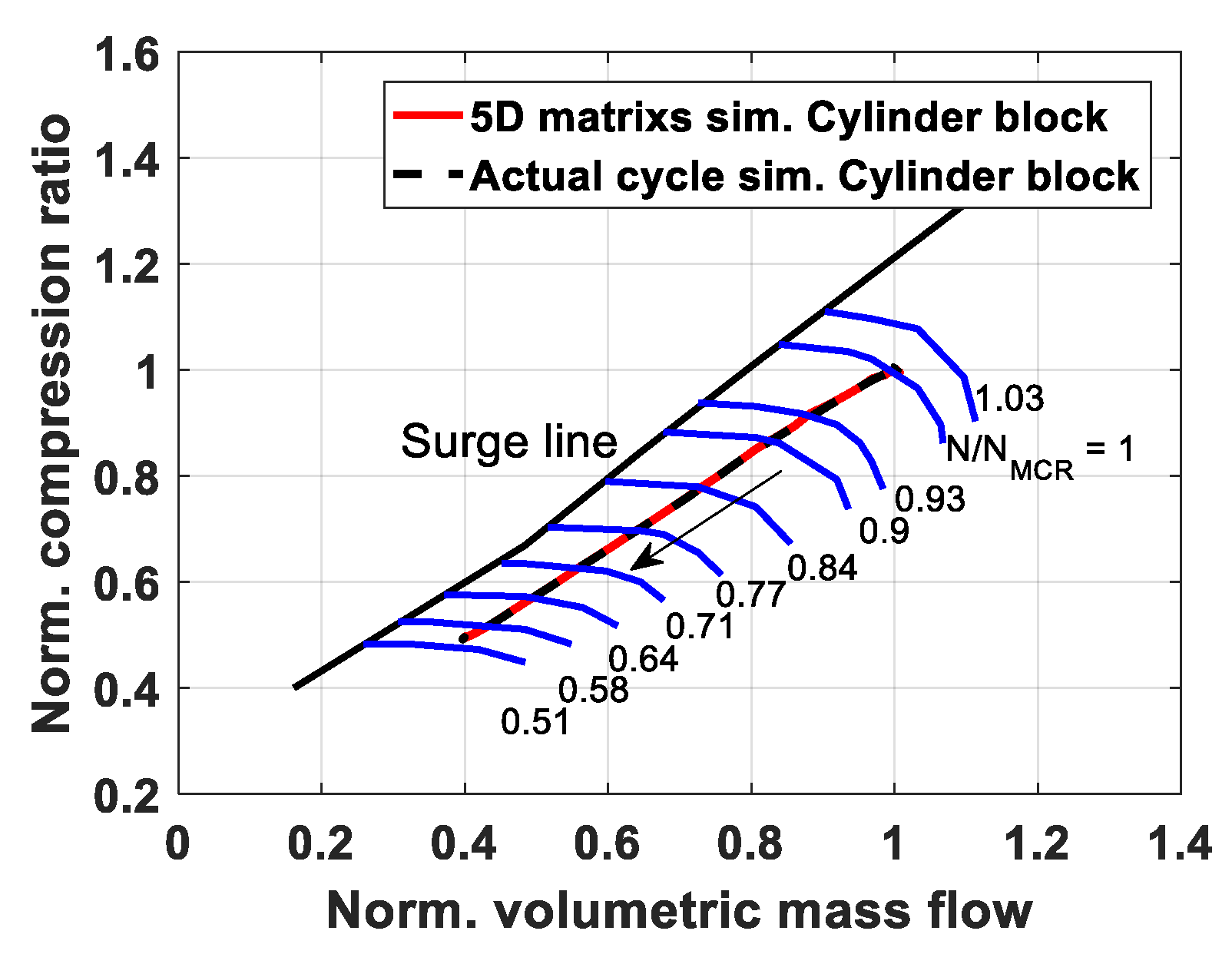
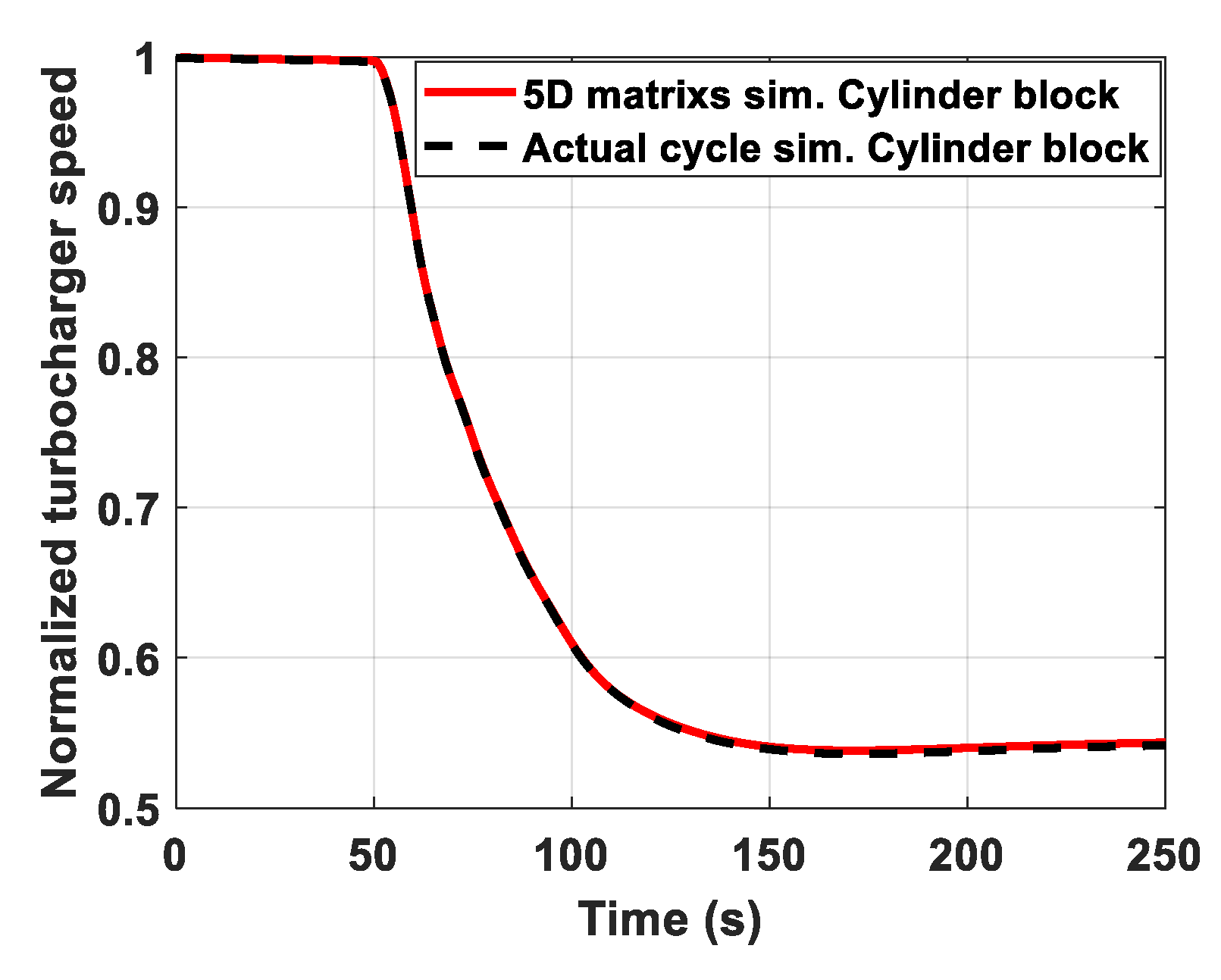
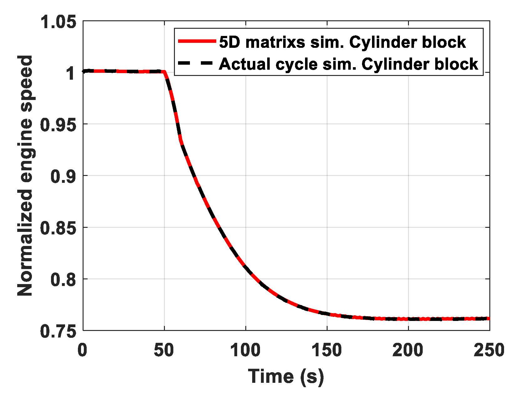
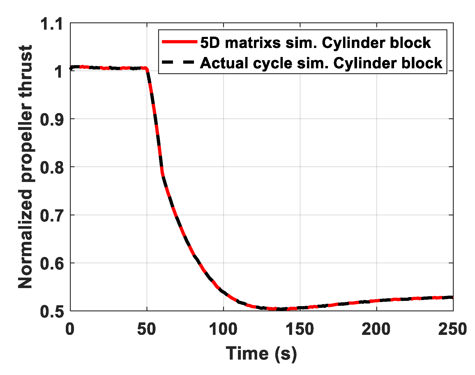
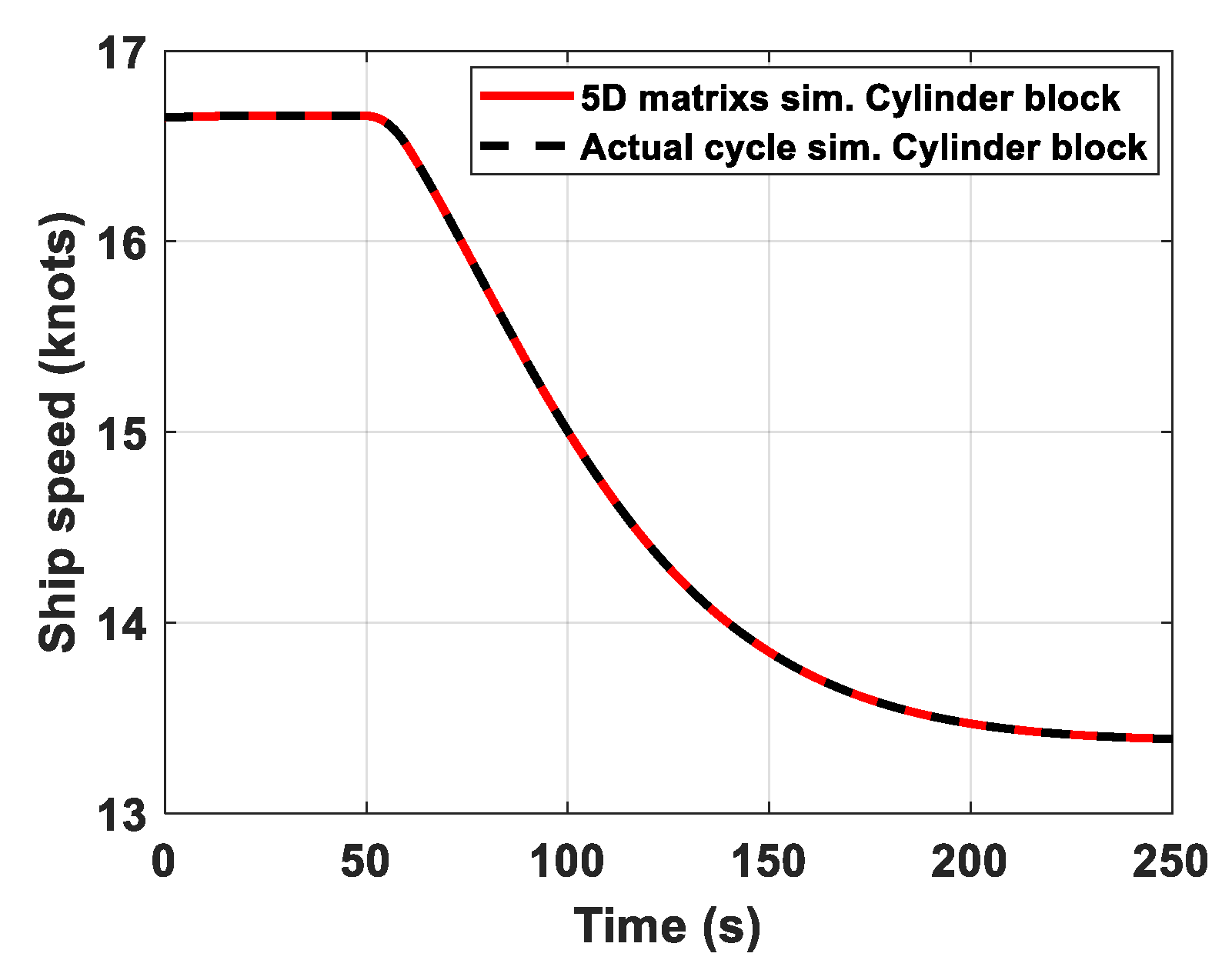
Figure 6 and
Figure 7 show simulation results in the engine working area and TC compressor map. The transient trajectories determined by the engine actual cycle cylinders model (dashed black lines) and 5-D matrices method (continuous red lines) are practically coincident. The same consideration can be substantially stated for the other engine and ship characteristics illustrated in
Figure 8,
Figure 9,
Figure 10,
Figure 11,
Figure 12,
Figure 13,
Figure 14,
Figure 15,
Figure 16 and
Figure 17. In detail, the two simulation approaches show larger differences in compression ratio (around 0.8%), air flow rate (around 0.5%), turbine inlet temperature (around 1%) and turbocharger rotational speed (0.6%).
A second transient example, considered for the two-engine simulator comparison, is a yacht deceleration due to the telegraph decrease from step 10 to four, as represented in
Figure 18.
Figure 19 shows the pertinent fuel mass flow rate percentage time variation.
In addition, from the point of view of the simulation running time, 250 s of the yacht acceleration manoeuvre are simulated in a MATLAB computation time of 206.95 s by the actual cycle “cylinders” engine model, versus the 2.04 s of the 5-D matrices approach. The ship deceleration needs to be performed by the simulation in 234.17 s and 2.06 s respectively for the two methods; similar results are found for other yacht propulsion manoeuvres. These speed data obviously depend on the particular computer processor power; therefore, the real noteworthy result is that the new simulation approach for the engine, in comparison with a traditional thermodynamic model, makes the whole ship simulator about one hundred times faster.
7. Conclusions
A methodology to simulate diesel engine dynamics is proposed in order to strongly reduce the simulation running time. The study stems from the need to use marine propulsion simulators in real time, specifically developed for control system design or training purposes. Thermodynamic equations, representing in-cylinder phenomena, are usually responsible for a high computation time, making the development of complex ship propulsion simulators in real time technically impossible. Hence the proposed approach is based on the steady state representation of the cylinder behaviour, through the introduction of 5-D matrices, each specifically built for the assessment of inlet air flow rate, engine torque, exhaust gas flow rate, pressure and temperature. By this method, the whole engine dynamics are mainly due to the turbocharger dynamics; in this regard, the simulation analysis carried out to reproduce the propulsion behaviour of a motor-yacht shows the validity of this assumption (turbocharger performance data show differences lower than 1% between the two simulation approaches). For the main result, the running time of the whole propulsion simulator is reduced by about 99% if the new approach for the engine dynamics description is adopted instead of the traditional one (based on the actual cycle in-cylinders calculation model). This faster computation speed allows to transform more easily the whole ship simulator into a real-time executable application, even if the complex aspects related to the representation of the vessel motions are considered. At the same time, the model is able to perform reliable engine dynamics in ship propulsion applications, providing also in-cylinder thermodynamic data.
In addition, the physical structure of the model allows to simulate similar diesel engines (characterized for example by a different number of cylinders) simply updating some geometrical data of turbocharger and manifolds. This kind of design option would be much more complicated to obtain in the case of using other numerical techniques such as neural networks (being essentially “black boxes” to be re-trained every time something is changed).
On the other hand, the method cannot disregard the availability of a fully thermodynamic model, necessary to numerically generate the five 5-D tables of the simplified approach. Moreover the ambient conditions effects (e.g., inlet air temperature) on the diesel engine performance can be more difficulty estimated without a complete thermodynamic model.
Therefore, although some drawbacks still exist in using this method, this research represents an effective answer to an important technical problem linked to the development of ship simulators in real-time.


