Storm Waves at the Shoreline: When and Where Are Infragravity Waves Important?

Abstract

Infragravity waves (frequency, f = 0.005–0.05 Hz) are known to dominate hydrodynamic and sediment transport processes close to the shoreline on low-sloping sandy beaches, especially when incident waves are large. However, in storm wave conditions, how their importance varies on different beach types, and with different mixes of swell and wind-waves is largely unknown. Here, a new dataset, comprising shoreline video observations from five contrasting sites (one low-sloping sandy beach, two steep gravel beaches, and two compound/mixed sand and gravel beaches), under storm wave conditions (deep water wave height, H₀ up to 6.6 m, and peak period, T_p up to 18.2 s), was used to assess: how the importance and dominance of infragravity waves varies at the shoreline? In this previously unstudied combination of wave and morphological conditions, significant infragravity swash heights (S_ig) at the shoreline in excess of 0.5 m were consistently observed on all five contrasting beaches. The largest infragravity swash heights were observed on a steep gravel beach, followed by the low-sloping sandy beach, and lowest on the compound/mixed sites. Due to contrasting short wave breaking and dissipation processes, infragravity frequencies were observed to be most dominant over gravity frequencies on the low-sloping sandy beach, occasionally dominant on the gravel beaches, and rarely dominant on the compound/mixed beaches. Existing empirical predictive relationships were shown to parameterize S_ig skillfully on the sand and gravel beaches separately. Deep water wave power was found to accurately predict S_ig on both the sand and gravel beaches, demonstrating that, under storm wave conditions, the wave heights and periods are the main drivers of infragravity oscillations at the shoreline, with the beach morphology playing a secondary role. The exception to this was the compound/mixed beach sites where shoreline infragravity energy remained low.

1. Introduction

1.1. Background and Literature

Infragravity (IG) waves (frequency f = 0.005–0.05 Hz) are known to play a crucial role in storm impacts such as overwashing and inundation [1], dune erosion and barrier breaching [2] and beach face erosion [3], becoming increasingly dominant toward the shoreline [4,5]. As such, gaining an understanding of their influence on hydrodynamics [6,7,8] and sediment transport is vitally important to sustaining coastal infrastructure.

In particular, the importance of IG waves in runup (the maximum vertical extent of wave uprush on the beach) was established on low-sloping sandy beaches [9]. Defined as the elevation of the shoreline above still water level, runup comprises a mean (set-up) and oscillatory component (swash) [10]. The swash transfers energy from the waves to the shore, playing a key role in sediment transport, and can drive significant erosion during storms [11]. Swash is often separated into infragravity and gravity (f = 0.05–1 Hz) frequency bands and quantified as significant swash height, S, equal to 4σ, where σ² is the vertical runup variance in each band. While infragravity swash was previously studied on a range of sandy beaches, how its importance varies on different beach types, and with different mixes of swell and wind-waves is currently unknown. Environmental conditions and significant infragravity swash height (S_ig), observed during 13 prominent experiments which underpin much of the understanding of infragravity swash processes on sandy beaches, are presented in

Table 1. Summary (range and mean) of environmental parameters and significant infragravity swash height (S_ig) sampled during previous research^.1. Subscript 0 indicates parameters calculated using deep water values, linearly deshoaled to 80 m water depth. N = number of observations; NC = North Carolina; CA = California; OR = Oregon; USA = United States of America.

Map No	Site/Experiment	Date	H0 (m)	Tp (s)	Tan β	D50 (mm)	ξ0	N	Sig (m)
1	Duck, NC (USA) Duck82	5–25 October 1982	0.7–4.1 1.71	6.3–16.5 11.9	0.09–0.16 0.12	0.75	0.68–2.38 1.44	36	0.4–2.4 1.2
2	Scripps, CA (USA)	26–29 June 1989	0.5–0.8 0.69	10–10 10	0.03–0.06 0.04	0.20	0.4–0.92 0.6	41	0.3–0.7 0.33
1	Duck, NC (USA) Duck90–Delilah	6–19 October 1990	0.5–2.5 1.40	4.7–14.8 9.3	0.03–0.14 0.09	0.36	0.44–1.70 0.90	138	0.4–1.7 0.91
4	San Onofre, CA (USA)	16–20 October 1993	0.5–1.1 0.8	13–17 14.9	0.07–0.13 0.1	-	1.6–2.62 2.2	59	0.5–1.8 0.96
3	Gleneden, OR (USA)	26–28 February 1994	1.8–2.2 2.1	10.5–16 12.4	0.03–0.11 0.08	-	0.26–1.2 0.9	42	0.9–1.9 1.4
5	Tersheling (Netherlands)	2–22 April 1994 1–21 October 1994	0.5–3.9 1.9	4.8–10.6 8.3	0.01–0.03 0.02	0.22	0.07–0.22 0.1	14	0.2–0.9 0.54
1	Duck, NC (USA) Duck94	3–21 October 1994	0.7–4.1 1.5	3.8–14.8 10.5	0.06–0.1 0.08	0.20–2.5	0.33–1.43 0.81	52	0.5–2.2 0.81
6	Agate, OR (USA)	11–17 February 1996	1.8–3.1 2.5	7.1–14.3 11.9	0.01–0.02 0.02	0.20	0.1–0.19 0.15	14	0.7–1.5 1.1
1	Duck, NC (USA) Duck97–SandyDuck	3–30 October 1997	0.4–3.6 1.3	3.7–15.4 9.5	0.05–0.14 0.09	0.90–1.66	0.34–3.22 1.1	95	0.3–1.8 0.88
7	Truc Vert (France)	3 March–13 April 2008	1.1–6.4 2.4	11.2–16.4 13.7	0.05–0.08 0.06	0.35	0.49–0.9 0.68	88	0.63–2.37 1.3
8	Tairua (New Zealand)	15–17 July 2008	0.7–1.0 -	9.9–12.5 11.0	0.09–0.13 -	0.4	1.4–2.25 -	25	0.6–0.95 0.75
9	Ngarunui (New Zealand)	8–9 November 2010	0.6–1.3 -	8.1–12.4 9.0	0.01–0.03 -	0.29	0.13–0.42 -	32	0.24–0.90 0.60
10	Somo (Spain)	4 May 2016	0.3–0.7 0.31	11.0–13.0 12.0	0.04–0.1 0.06	0.28–0.35	0.9–2.5 1.5	12	0.28–0.90 0.57

^1. Further information and datasets are available for sites 1–6: https://pubs.usgs.gov/ds/602/#intro; site 7 [6]; site 8 [14]; site 9 [15]; and site 10: https://data.mendeley.com/datasets/6yh2b327gd/4.

, and their locations and relative exposure are provided in Figure 1. Mean values were obtained from Reference [12] and ranges from Reference [13]. Further information and reference to published works relating to the data in Table 1 can also be found in Reference [10].

Table 1 and Figure 1 highlight the combined importance of incident wave height and period to infragravity response at the shoreline. The four experiments where mean values of S_ig exceeded 1 m were exposed, including open ocean sites, where both wave height and period were large (Duck82, Glenderon, Agate (Figure 1b), and Truc Vert (Figure 1c)). In contrast, despite large wave heights (H₀ up to 3.9 m), short wave periods (mean T_p 8.3 s), typical of the fetch limited Tersheling (Figure 1c), resulted in a low mean S_ig of 0.54 m.

In an attempt to understand the conditions which result in infragravity frequencies becoming important in the swash, much of the sandy beach data presented in Table 1 were used to try and establish empirical relationships between S_ig, wave statistics, and beach gradient. One of the first attempts to parameterize S_ig in this way was that of Reference [16], which demonstrated that monochromatic wave runup scaled well with the Iribarren number.

ξ = tan β/(H₀L₀)^1/2,

(1)

where tan β is the beach gradient, and H₀ and L₀ are the deep water (offshore) significant wave height and wavelength, respectively. The Iribarren number represents a dynamic beach steepness comparing beach slope to wave steepness, with the application of Equation (1) to natural datasets facilitating the examination of runup in a morphodynamic parameter space [17]. As such, the terms in Equation (1) form the basis of many runup and (more specifically) swash predictors.

The pioneering work of Reference [18] demonstrated a contrasting relationship between H₀ and horizontal swash in the gravity and infragravity band, whereby swash was seen to be saturated in the gravity band but increased linearly with H₀ in the infragravity band. Other researchers since reported a similar linear relationship between vertical significant infragravity swash height (S_ig) and H₀, with a range of constants of proportionality [6,19,20].

Attempting to find a universal parameterization of S_ig, applicable to a range of sandy beaches, Reference [10] found that including a wavelength term, (H₀L₀)^1/2, improved predictions of S_ig, a result corroborated under high energy conditions observed at a single site by Reference [6]. While effective at parameterizing infragravity energy in the swash, Reference [8] found that, at an exposed sandy site, a stronger correlation existed between infragravity wave height in the surf zone and H₀²T, citing its proportionality to deep water wave power as more physically correct than Stockdon’s (H₀L₀)^1/2.

While observations focusing specifically on infragravity swash are almost entirely limited to sandy environments, an example of similar research on gravel beaches is that of Reference [17], which, without focusing specifically on infragravity frequencies, assessed runup elevation under extreme conditions, on a range of gravel beaches. The authors found that existing runup predictors developed on sandy beaches, including that of Stockdon, under-predicted runup elevation on gravel beaches, instead finding that (tan β^1/2H₀T_p) provided a more accurate estimate.

Observations of infragravity swash under storm wave conditions are limited to a small number of experiments carried out on sandy beaches, as discussed in Section 1.1 and presented in Table 1. Furthermore, infragravity swash behavior is yet to be compared on sand, gravel, and mixed sediment beaches.

1.2. Scope of Research

The present research stands in contrast to previous contributions by observing infragravity waves in a wide range of high-energy swell and wind-wave conditions across a range of beach morphologies and grain sizes not previously explored. Here, video observations of the shoreline under storm wave conditions (H₀ up to 6.6 m and T_p up to 18.2 s) were collected at four contrasting beaches in the south of the United Kingdom (UK). These were complemented by previously published data from one additional site, to produce a unique and novel dataset comprising observations of storm waves on one sandy beach, two gravel beaches, and two compound/mixed sand and gravel beaches.

The present work aims to assess how the importance and dominance of infragravity waves varies at the shoreline by doing the following:

• Compiling a dataset comprising observations in previously unrecorded combinations of wave and morphological conditions;
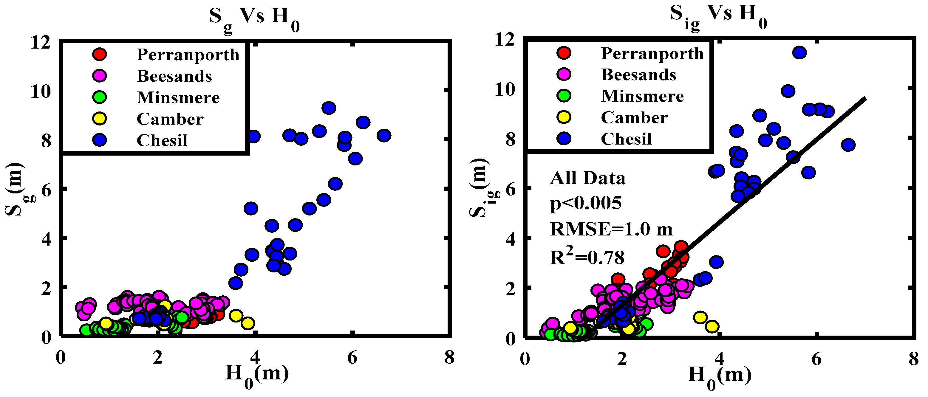
• Assessing how swash height in the gravity (S_g) and infragravity bands (S_ig) relates to offshore wave height (H₀);
• Examining how accurately previous parameterizations of S_ig, developed over a limited range of wave and morphological conditions, can be used to predict S_ig across the range of morphologies in the new dataset, and whether an improved parameter can be obtained;
• Developing a conceptual model to illustrate the importance of infragravity swash at the shoreline on a wide variety of beach morphologies under a wide range of high-energy swell and wind-wave combinations.

2. Materials and Methods

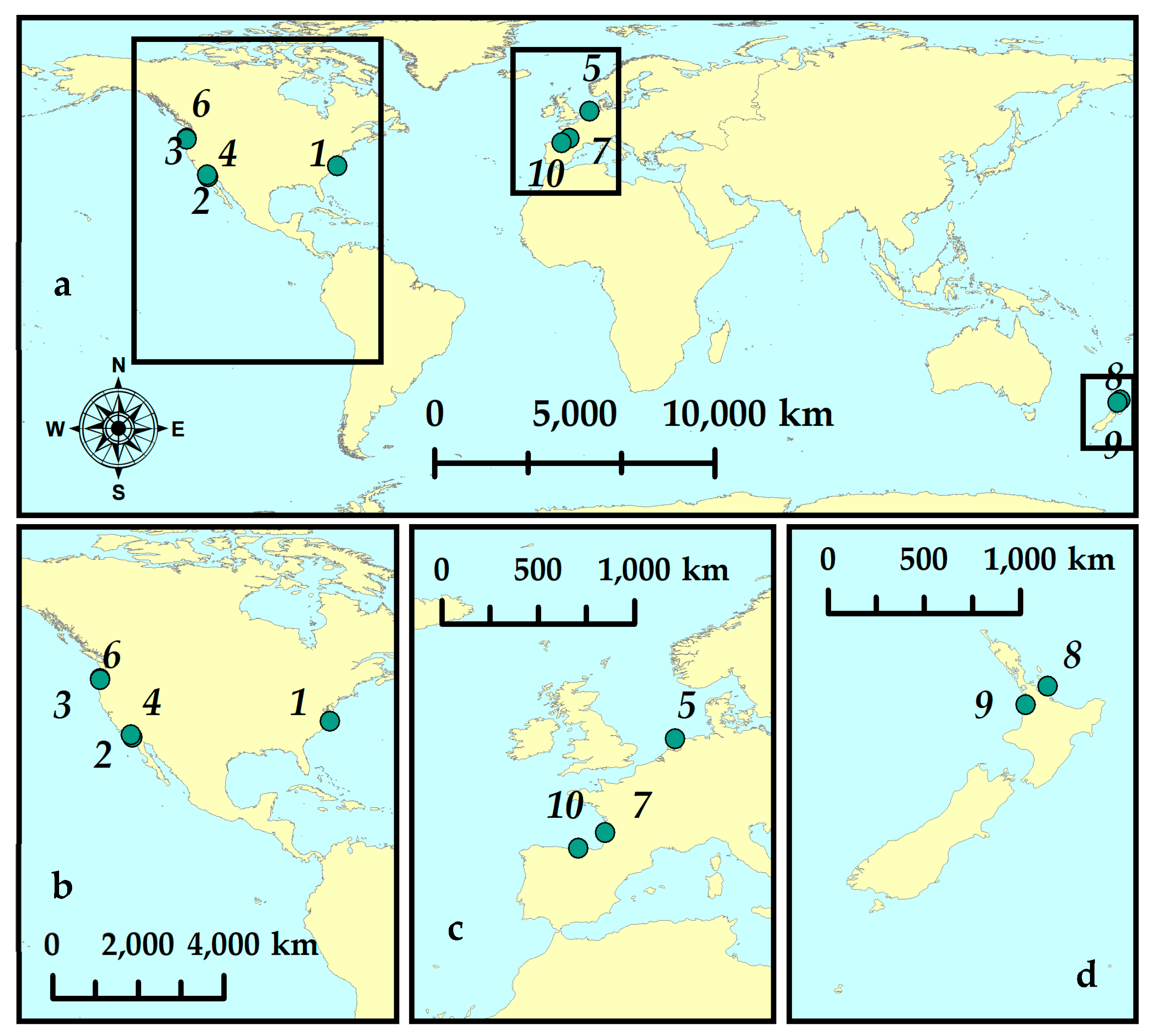
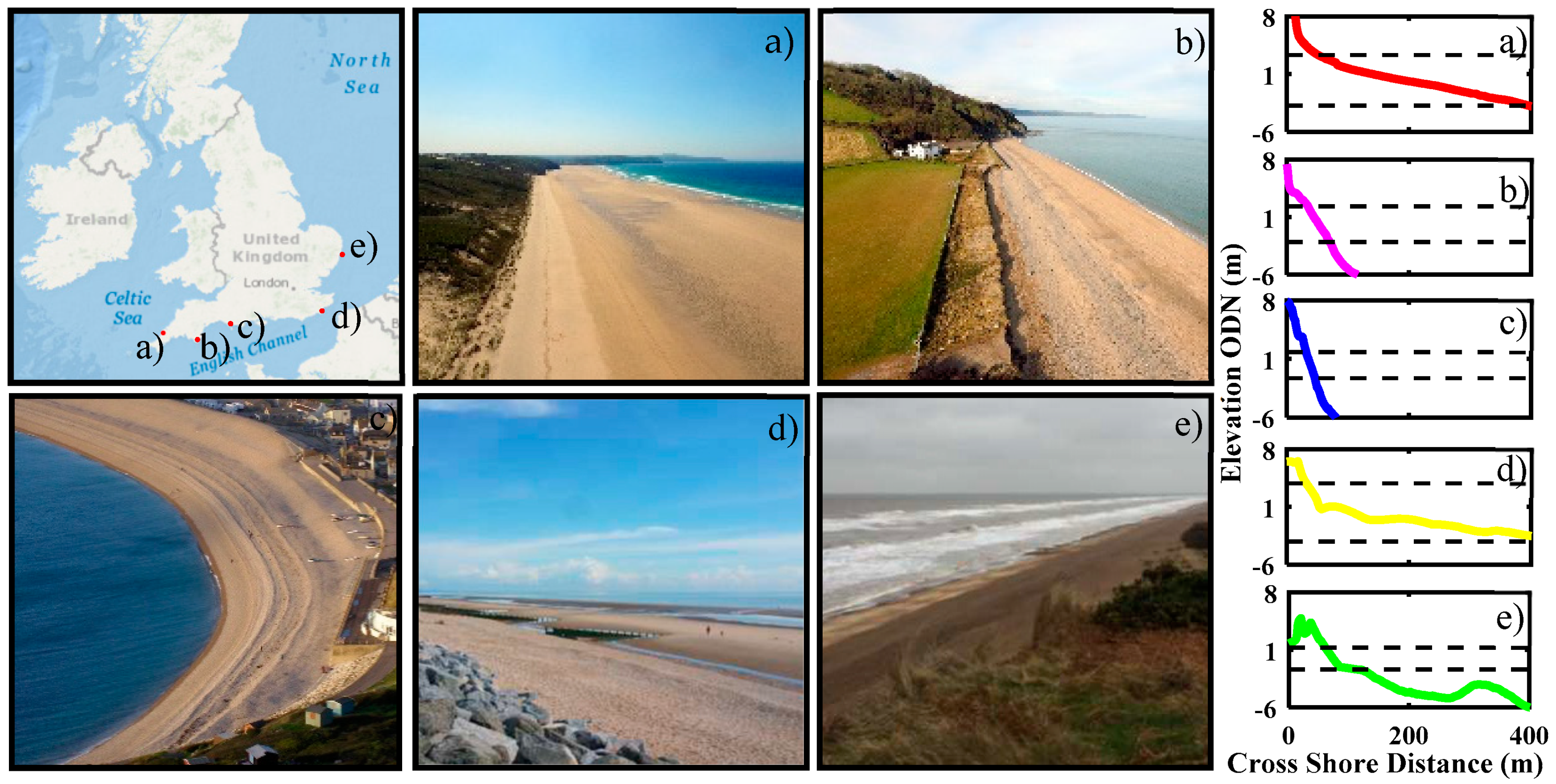
2.1. Description of Field Sites

Five beaches in the south of England, UK, were specifically selected as study sites owing to their contrasting wave climates, and morphology (Figure 2a–e). From west to east, the sites included one low-sloping sandy beach, Perranporth (PPT), two steep gravel beaches, Beesands (BEE) and Chesil (CSL), and two compound/mixed sand and gravel sites, Camber (CAM) and Minsmere (MMR). These two sites can be divided, according to the classification of Reference [21], into a composite beach (CAM) and a mixed sand and gravel beach (MMR).

Quality-controlled, 30-min averages of significant wave height (H_s) and wave period (T_p) at each of the five sites collected at local “directional wave rider” buoys were downloaded from channelcoast.org. This time series of H_s and T_p was then linearly interpolated to obtain values every 20 min, consistent with the length of data runs measured at the shoreline (Section 2.2). Located within 5 km of the relevant beach, mean depths at the wave buoys ranged from 9.8 to 23 m. Consistent with the examples in Table 1, estimates of offshore significant wave height (H₀) were obtained by linearly deshoaling H_s to a depth of 80 m. The range and mean H₀ and T_p observed during data collection at each of the five sites are listed in

Table 2. Site descriptors, storm name, and return period in years; 95% exceedance threshold offshore wave height (H_{_95}) and period (T_{p_95}), and the range of H₀ and T_p in the new dataset were collected, with maximum values quoted in bold.

Site	Description	Storm Name Date Return Period (Years)	H0_95 (m)	H0 (m) Range	Tp_95 (s)	Tp (s) Range	ξ0 Typical Range *
Perranporth (PPT)	High-energy, dissipative sandy beach, exposed to oceanic swell and locally generated wind waves	Unnamed storm 31 January–7 February 2017 1 in 1	3.1	1.6–3.2	15.4	11.1–18.2	0.14–0.33
Chesil (CSL)	Medium-energy, reflective gravel beach, partially exposed to oceanic swell and locally generated wind waves	“Petra” 5–6 February 2014 1 in 10	2.6	1.6–6.6	15.3	10.3–16.7	1.1–5.5
Beesands (BEE)	Low-energy, reflective gravel beach, dominated by wind waves and occasional refracted oceanic swell	“Beast from the east/Emma” 20–27 February 2018 1 in 60	1.9	0.4–3.3	14.3	5.1–15.0	0.5–2.4
Camber (CAM)	Low-energy, fetch-limited, compound beach with steep gravel upper and low slope sandy terrace	“Angus” 4–6 November 2016 1 in 10	2.0	0.9–3.8	11.1	5.5–10.0	0.06–1.5
Minsmere (MMR)	Low-energy, fetch-limited, mixed sand and gravel beach. Steep upper shore face, low slope below low water. Submerged offshore bar	Unnamed storm 6–8 January 2018 1 in 5	1.9	0.52–2.5	8.3	3.3–7.7	0.14–1.5

* Typical range of ξ₀ taken as the average value of ξ_0, calculated over the data record at each wave buoy, ±1 standard deviation. Representative slope(s) (tan β) were selected per site as follows: PPT = 0.02; BEE = 0.1; CSL = 0.25; CAM = 0.02 (lower), 0.1 (upper); MMR = 0.03 (lower), 0.13 (upper). For the sites with two slopes, the lower value was used to calculate the lower end of the range, and the upper value to calculate the upper value.

. Maximum values are placed in bold to emphasize the unique experimental conditions.

In order to define wave conditions as “extreme”, 95% threshold values of offshore wave height (H_{0_95}) and period (T_{p_95}) were calculated, a statistic frequently used to define storm events [22]. The full data record at each local wave buoy, which in all cases was at least six years in length, was used to calculate H_{0_95} and T_{p_95} (Table 2). This statistic facilitates comparison of observed wave conditions between sites of contrasting exposure. Waves in excess of the 95th percentile H₀ were observed at all five sites, with particularly extreme named storm events being observed at Beesands (“Emma”), Camber (“Angus”), and Chesil (“Petra”), where mean H₀ for the entirety of the experiment exceeded the 95th percentile (Table 2). T_{p_95} was exceeded at three of the five sites (Perranporth, Chesil, and Beesands) which were susceptible to swell. Furthermore, comparing Table 1; Table 2, it can be seen that the largest H₀ (6.6 m at Chesil) and the largest T_p (18.2 s at Perranporth) in the new dataset exceeded the maximum values in Table 1 (H₀ = 6.4 m at Truc Vert) and (T_p = 16.5 s at Duck 82). This demonstrated that highly unusual wave heights and periods were observed during all five deployments, an innovative aspect of this work.

Typical ranges of ξ₀, calculated to indicate the prevailing wave breaking regime at each site using Equation (1), are presented in Table 2. Breaker types as defined by Reference [23] were taken as surging (ξ₀ > 3.3), plunging (0.5 < ξ₀ < 3.3), and spilling (ξ₀ < 0.5). It can be seen that Perranporth, the low-sloping sandy beach, is typically dominated by spilling breakers. At the mixed/compound sites, breakers are typically spilling or plunging. On the steep gravel beaches, breakers range between plunging at Beesands to plunging and surging at Chesil.

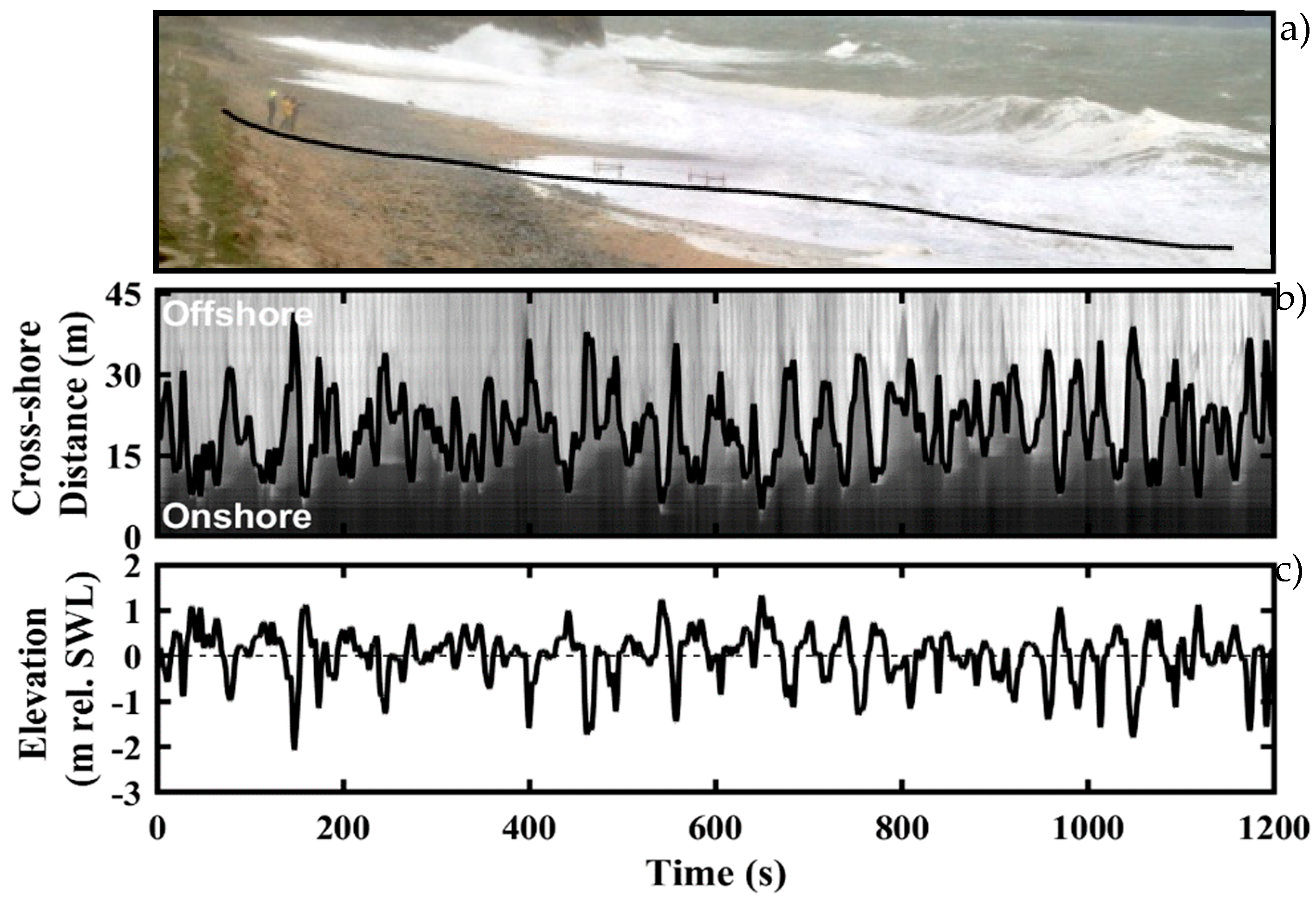
2.2. Field Data Collection and Video Data Processing

At each of the sites, data collection was targeted around storm events using Plymouth University’s Rapid Coastal Response Unit (RCRU). The RCRU is a versatile and sheltered base, facilitating the collection of hydrodynamic and topographic data during extreme storms. Housing an array of in situ and remote instrumentation, the unit is highly mobile and can be deployed with just an hour’s notice, in order to capture the approach, peak, and decay of a storm [24,25,26]. In the present example, a 10-m tower, equipped with high-resolution video cameras, fed data to a computer inside the RCRU, storing over 70 h of video images across the five deployments.

At all sites, a representative cross-shore profile (“analyzed profile”, Figure 3a) was carefully selected to monitor runup, minimizing the impact of longshore sediment transport, headlands, or sea defenses on the beach profile. Daily monitoring of the profile was carried out using real-time kinematic global positioning system (GPS), capturing changes every other low tide. A value of beach slope (tan β) was defined per 20-min data run as the average gradient between the 2% exceedance level of runup (R2%) and still water level (SWL), minus twice the offshore significant wave height (SWL − 2H₀), following Reference [17].

In order to calculate swash statistics, images captured at a rate of 4 Hz by a Pointgrey Grasshopper camera fitted with a 25-mm lens were used to produce pixel stacks as follows. Ground control points, where both the real-world and image positions were known, were used to generate a geometry solution, facilitating conversion of coordinates from a two-dimensional (2D) (U, V) image to a three-dimensional (3D) (X, Y, Z) real-world system and vice versa. The method used here for obtaining photogrammetric relationships was developed by Reference [27] and is widely used in comparable works [6,10,17]. The line of pixels corresponding to the “analyzed profile” (Figure 3a) was extracted from each image and stacked horizontally against time. The blue−red ratio and intensity of each pixel was evaluated, and threshold values defined those which corresponded to the discrete transition from dry beach to swash, after Reference [10], yielding a digitized time series of swash. Finally, this was converted from UV to XY space to produce a time series of horizontal swash (Figure 3b), with the elevation (Z) associated with each cross shore position used to quantify vertical swash height (Figure 3c). Eight-point unweighted sliding-average frequency-smoothed spectral estimates were computed for each 20-min time series of vertical swash (Figure 4b,d,f,h,j), each with 16 degrees of freedom. The same frequency smoothing was applied to the offshore spectral estimates (Figure 4a,c,e,g,i). These were calculated using 20-min time series of raw surface elevation, collected at local wave buoys. Spectral variance was used to calculate total significant swash height (S) and separate incident (S_g) (f = 0.05–0.3 Hz) and infragravity (S_ig) (f = 0.003–0.05 Hz) band heights according to Equation (2).

S = 4√∑^f2_f1 PSD(f)Δf

(2)

where f1 and f2 are the upper and lower frequency bounds of S, S_g, or S_ig, PSD is power spectral density, f is frequency, and Δf is bandwidth in Hz.

3. Results

3.1. Enviornmental Conditions

Data collection was targeted around extreme storm wave events at each of the five sites, summarized in

Table 3. Summary (range and mean) of environmental parameters sampled during the presented research. Subscript 0 indicates parameters calculated using deep water values linearly deshoaled to 80 m depth. N = number of 20-min data runs; UK = United Kingdom.

Site/Experiment	Date	H0 (m)	Tp (s)	Tan β	D50 (mm)	ξ0	N	Sig (m)
Beesands, UK	20–27 February 2018	0.4–3.3 2.0	5.1–15.0 7.4	0.09–0.11 0.10	- 5	0.53–2.84 0.71	75	0.20–2.3 1.3
Perranporth, UK	31 January–7 February 2017	1.6–3.2 2.4	11.1–18.2 15.7	0.02–0.08 0.034	- 0.25	0.19–0.96 0.44	31	1.1–3.6 2.2
Camber Sands, UK	5–6 November 2016	0.9–3.8 2.2	5.5–10.0 7.7	0.02–0.10 * -	0.33–10 * -	0.059–1.1 1	16	0.30–0.81 0.53
Minsmere, UK	6–8 January 2018	0.52–2.5 1.6	3.3–7.7 6.4	0.03–0.13 ** -	0.33–20 ** -	0.1–0.97 0.21	43	0.01–0.68 0.33
Chesil, UK	5–6 February 2014	1.6–6.6 3.9	10.3–16.7 13.8	0.24–0.38 0.32	65 -	2.21–3.84 3.7	40	0.65–11.4 5.1

* Camber is a compound beach with a steeper gravel upper and low-slope sandy lower; ** Minsmere is a mixed sand and gravel site (as reflected in the wide-ranging D₅₀ with a steep gravel upper and lower-sloped lower profile.

. At Chesil, both exceptionally long-period waves (<16.7 s) in excess of the 95th percentile and shorter-period swell waves (>10 s) yielded a mean period of 13.8 s. Perranporth was dominated by exceptionally long-period swell waves with mean T_p (15.7 s) in excess of the 95th percentile threshold. At Beesands, two days of small swell waves extended the upper limit of observed T_p to 15 s. However, the comparatively low mean T_p (7.4 s) demonstrates that the deployment was dominated by locally generated wind waves. Deployments at Minsmere and Camber were characterized by large wind waves, as reflected in the mean periods of 7.7 s and 6.4 s, respectively.

Of the five sites, the largest significant infragravity swash height (S_ig) (11.4 m) and largest mean S_ig (5.1 m) were observed at Chesil. The extreme heights can be explained by the exceptionally high beach slope (tan β < 0.38) and wave heights (H₀ < 6.6 m) and are comparable to the exceptionally high runup values obtained by Reference [17] during the same experiment (R2% up to 13 m). The second largest S_ig heights were observed at Perranporth, a site more typically associated with infragravity dominance. While the mean (2.2 m) and largest (3.6 m) observed S_ig were smaller than observed at Chesil, Perranporth was the only site where S_ig was always above 1 m. Significant levels of infragravity energy were also present in the swash at Beesands, where S_ig heights of up to 2.3 m and a mean height of 1.3 m were observed. The lowest S_ig heights were observed at the compound/mixed sand and gravel sites, Camber and Minsmere, where the maximum S_ig (0.81 and 0.68 m, respectively) was lower than mean S_ig observed at any other site.

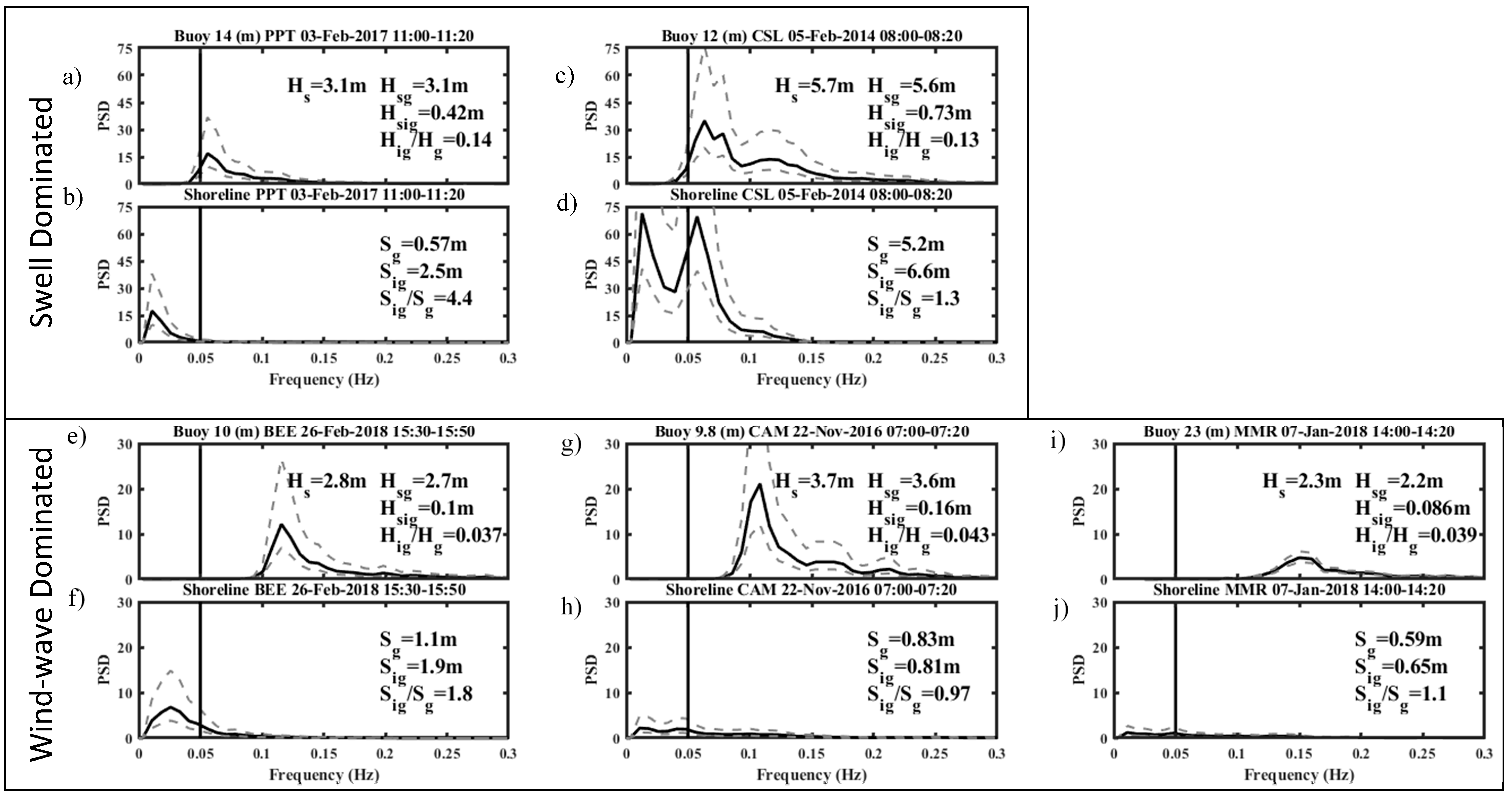
3.2. Comparison of Spectra at Wavebuoy and Shoreline

Offshore spectra calculated at local wave buoys (Figure 4a,c,e,g,i) were compared to those calculated at the shoreline from time series of vertical swash (Figure 4b,d,f,h,j). The examples presented in Figure 4 were specifically selected as most clearly representing extreme conditions at each site. Times where H_{0_95} was exceeded coinciding with high water (±1.5 h) were targeted in order to minimize contamination of the spectra with tidal signal.

The buoy spectra can be divided into swell-dominated (Perranporth and Chesil, Figure 4a,c, respectively) and wind-wave-dominated (Beesands, Camber and Minsmere, Figure 4e,g,I, respectively).

At the shoreline, spectra can be divided into three groups: infragravity-dominated due to dissipation of gravity energy and growth of IG energy (Perranporth and Beesands, Figure 4b,f, respectively); high-energy gravity and infragravity due to minimal dissipation (Chesil, Figure 4d); low energy in both bands, due to maximum dissipation (Camber and Minsmere, Figure 4h,j, respectively).

At Perranporth, a single, significant peak in the gravity band of the wave buoy spectrum (0.056 Hz, 17.9 s) (Figure 4a) was replaced by a single significant peak in the infragravity band in the shoreline spectrum (0.011 Hz, 90 s) (Figure 4b). As a result, significant gravity swash height (S_g = 0.57 m) remaining at the shoreline was less than one-fifth of the offshore wave height in the gravity band (H_sg = 3.1 m), and infragravity swash (S_ig = 2.5 m) was roughly six times larger than offshore infragravity height (Hs_ig = 0.42 m).

At Chesil, a single incoming peak (0.063 Hz, 15.8 s) in the gravity band of the wave buoy spectrum (Figure 4c) was maintained in the shoreline spectrum (Figure 4d). In addition, an IG peak at 0.013 Hz (77 s) was also present in the shoreline spectrum (Figure 4d). Significant wave and swash height were similar in the gravity band (H_sg = 5.6 m, S_g = 5.2 m) and increased by an order of magnitude between the buoy and the shoreline in the IG band (H_sig = 0.73 m, S_ig = 5.2 m).

The contrast in development of spectra between the buoy and the shoreline at Perranporth and Chesil resulted from differences in short wave breaking and dissipation. At Perranporth, incoming swell waves were efficiently dissipated across a wide surf zone as spilling breakers. At Chesil, dissipation of swell waves appeared to be minimal. The steep beach face and large, low-steepness incoming waves resulted in high-energy surging and plunging breakers breaking directly on the beach face as a shore break, conserving the swell peak in the shoreline spectrum.

At the wind-wave-dominated sites, a reduction in total energy from the buoy to the shoreline indicated energy dissipation, where steep storm waves produced spilling breakers on the shallow lower profile of the compound/mixed sites (Minsmere and Camber) and plunging breakers on the gravel site (Beesands).

At Beesands the shoreline spectrum (Figure 4f) shows that energy at gravity band frequencies (incident wave peak, 0.12 Hz, 8.3 s) was dissipated with growth of a broad low-frequency peak at 0.026 Hz (38 s). In the gravity band, swash height (S_g = 1.1 m) reduced to around half that of H_sg (2.7 m), and the infragravity band swash height (S_ig = 1.9 m) was around 20 times larger than H_ig (0.10 m).

At Camber (Figure 4g) and Minsmere (Figure 4i), the majority of the incoming short wave energy (concentrated at wind-wave frequencies of around 0.11 Hz (9.1 s) and 0.15 Hz (6.0 s), respectively) was dissipated by the shoreline. This resulted in an absence of energy in the gravity band and a single low-energy, low-frequency peak in the shoreline spectra of both sites (Figure 4h,j).

3.3. Reletionship between Swash and Offshore Wave Height (H₀)

Linear regression was used to assess the relationship between swash and offshore wave height, where a significant relationship at the 99.5% confidence limit was given by (p < 0.005). Goodness of fit was summarised by correlation squared (R²) and root mean square error (RMSE) and the relationship quantified by regression slope (m) and y-axis intercept (c). Partitioning vertical significant swash height into the gravity (S_g) and infragravity (S_ig) bands highlighted their contrasting relationship with increasing offshore significant wave height (H₀) (Figure 4, left and right respectively). Regression statistics for the relationship between S_ig and H₀ at each of the sites individually and all sites combined are summarised in

Table 4. Relationship between significant swash in the infragravity band (S_ig) and offshore wave height (H₀). RMSE = root-mean-square error.

Site	Regression Slope (m)	Intercept (c)	R2	p	RMSE (m)
CSL	2.02	−2.82	0.86	<0.005	1.29
PPT	1.06	−0.40	0.67	<0.005	0.44
BEE	0.51	0.30	0.65	<0.005	0.28
MMR	0.25	−0.06	0.67	<0.005	0.11
CAM	0.04	0.44	0.03	0.51	0.16
Combined	1.66	−2.01	0.78	<0.005	1.00

.Significant swash height in the gravity band (S_g) showed no significant increase with H₀ (p > 0.005) at all sites (except Chesil), implying saturation in the gravity band. As such, no line of best fit is shown in Figure 5 (left). At Chesil, the increase of S_g with H₀ shows that the gravity band was not saturated, resulting in large amounts of energy in the gravity band reaching the shoreline during large offshore wave conditions.

In contrast, significant swash height in the infragravity band (S_ig) showed significant (p < 0.005) and well-correlated relationships (R² = 0.65–0.86) with H₀ at all sites (except Camber, where p = 0.51), showing that S_ig at the shoreline continued to increase with increasing H₀. The diversification in behavior of swash in the gravity and infragravity band at all sites except Chesil shows that an increase in offshore wave height (H₀) has no influence on gravity band swash heights, but leads to a linear increase of infragravity band swash heights. This implies that swash heights in the gravity band are saturated as a result of shortwave dissipation.

Both the largest offshore wave (H₀ < 6.7 m) and shoreline infragravity swash heights (S_ig < 11.4 m) were observed at Chesil, resulting in the steepest regression slope (m = 2.0). The next largest S_ig heights were observed at Perranporth where S_ig ranged between 2.5 and 3.2 m for H₀ = 2.5–3.6 m, over twice the S_ig heights (1.4–2.6 m) observed over the same range of H₀ at Beesands. Despite their contrasting regression slopes, Chesil (m = 2.02), Beesands (m = 0.51), and Perranporth (m = 1.1) showed comparable S_ig heights (0.75–2 m) when H₀ ranged between 1.5 and 2.5 m.

The dataset as a whole showed a strong and significant linear correlation between S_ig and H₀ (p < 0.005, R² = 0.78), with a regression slope (m) of 1.7 and an intercept (c) of −2.0. The negative value of c caused the line of best fit to intercept the x-axis, facilitating the tentative definition of a threshold of H₀ of around 1.3 m, above which infragravity energy becomes apparent in the swash.

The spread of values of S_ig for a given value of H₀ at Chesil may be attributed to variability in the incoming wave conditions and/or the profile and beach slope over which waves were breaking and running up. It is feasible that values of H₀ varied within a given 20-min run, resulting in variability in S_ig, owing to the linear relationship described in Figure 5. Furthermore, gravel morphology is known to respond rapidly to wave forcing [28]; thus, the assumption of a constant slope throughout a tidal cycle may not be representative of reality.

The relative contributions of infragravity and gravity energy to the swash were assessed using the ratio S_ig/S_g, where values greater than (less than) one imply infragravity (gravity) dominance. Figure 5 shows the ratio of S_ig/S_g plotted against H_0.

Perranporth was most dominated by infragravity swash, with an S_ig/S_g ratio of up to 4.4 for the largest incident wave conditions, H₀ = 3.2 m (Figure 5). At Chesil, despite the absolute magnitude of S_ig being largest at this site (Figure 4, right), values of S_ig/S_g were smaller and varied between 0.7 and 2.5 across the entire observed range of wave heights (H₀ = 1.6–6.8 m). The difference in infragravity dominance at the two sites can in part be explained by the contrasting short wave dissipation pattern shown in Figure 4 (left). Spilling breakers dissipated much of their energy across the wide surf zone, resulting in saturated values of S_g at Perranporth. In contrast, high-energy plunging and surging breakers produced a shore break on the steep beach face at Chesil, resulting in a lack of dissipation and S_g increasing linearly with H₀.

Infragravity dominance increased with offshore wave height (H₀) at Beesands. However, it can be seen from Figure 6 that S_ig/S_g at Beesands increased at a lower rate than Perranporth, implying that, for a given wave height, infragravity frequencies were less dominant. Unlike at Perranporth, short wave dominance (S_ig/S_g < 1) was observed at Beesands. At this site specifically, a transition from gravity-dominated to infragravity-dominated swash occurred at a threshold of H₀ 1.5 m.

At Minsmere, the ratio of S_ig/S_g increased with low values of H₀ (<1.3 m) but, crucially, barely exceeded 1, signifying gravity dominance. At Camber, no relationship with H₀ was apparent, with the maximum observed ratio of S_ig/S_g = 0.9. This clearly demonstrated that, even during large waves (H₀ > 1.3 m), infragravity frequencies rarely became dominant over gravity frequencies in the swash on the compound/mixed beaches.

3.4. The Role of Wave Height, Period, and Beach Slope

In addition to wave height, previous research highlighted the potential importance of wave period and beach slope in the prediction of significant infragravity swash height (S_ig). As such, in Section 3.4.1, Section 3.4.2 and Section 3.4.3, three predictors of S_ig are applied to the presented new dataset and the strength of relationship assessed using linear regression and bias as follows:

Bias = ∑(x_predicted − x_observed)/n,

(3)

where n represents the number of observations in both x_predicted and x_observed.

In addition to the combinations of wave and beaches statistics presented in Section 3.4.1, Section 3.4.2 and Section 3.4.3 ((H₀L₀)^0.5, (tan β)^0.5 H₀T_p, (H₀²T)), the following parameters were tested and were found to show weak or no significant relationship with S_ig: tan β(H₀L₀)^0.5, (tan βH₀L₀)^0.5, (tan β)^0.5, and (tan β)^0.5H²T; as such, they are not presented.

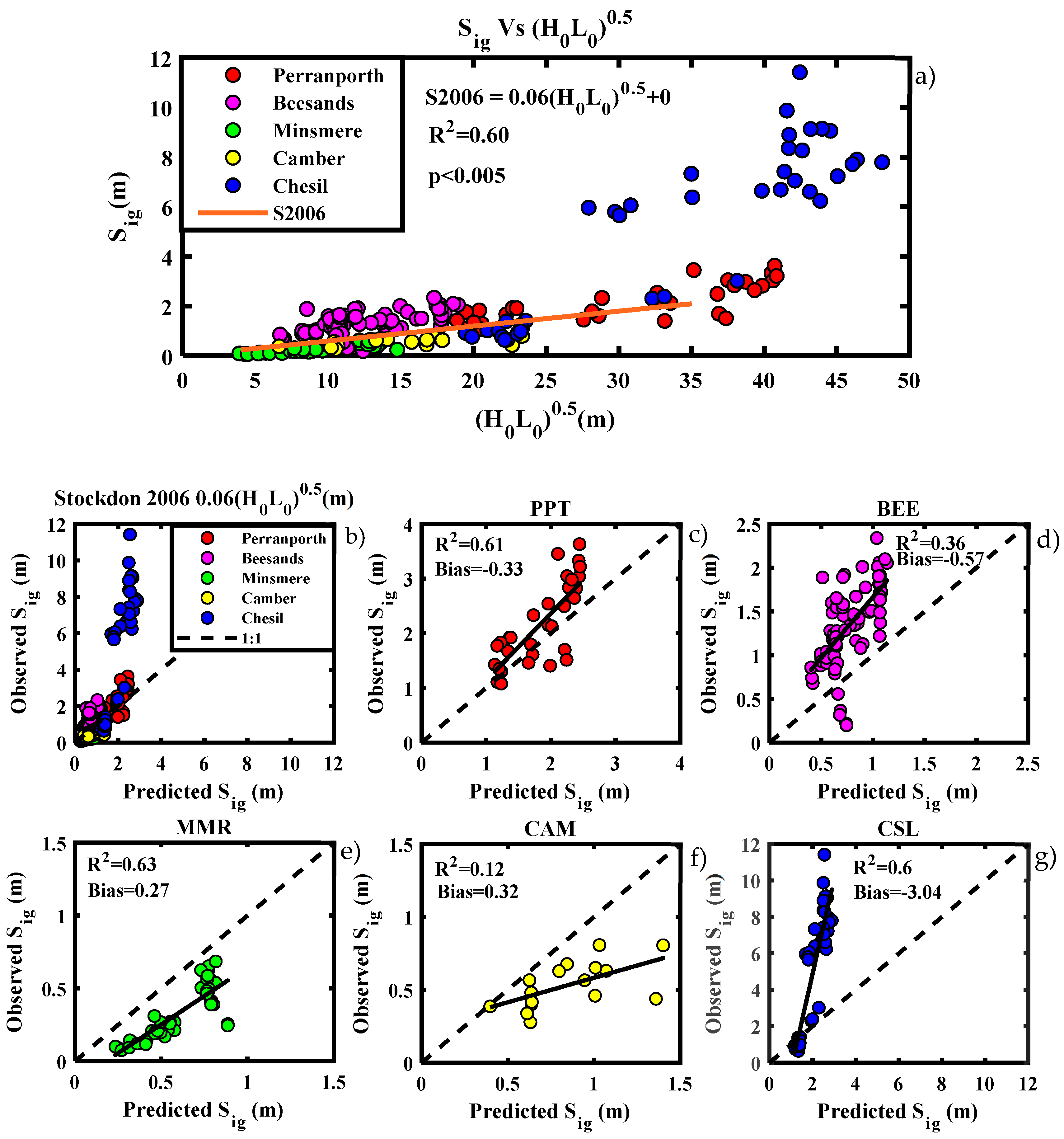
3.4.1. Stockdon (S2006)—Sandy Beaches

Equation (4) [10] (S2006) was developed empirically using a range of data from 10 sandy beaches.

S_ig = 0.06(H₀L₀)^0.5,

(4)

where H₀ is the deep water wave height and L₀ is the deep water wave length. Note that Stockdon forced the intercept (c) through the origin.

S_ig observed at our five sites was plotted against (H₀L₀)^0.5 to assess how the relationship compared with Stockdon’s observations (Figure 7a), yielding a significant correlation (p < 0.005) at all sites except Camber, with a variety of regression slopes.

S_ig at Perranporth (red points) plotted well with the S2006 equation (orange line) over a comparable range of (H₀L₀)^0.5 (20–35 m), which was an unsurprising result, given the similarity of Perranporth to the beaches in Stockdon’s dataset. The majority of the Beesands data plotted above the S2006 line (Stockdon under-predicting), while the compound/mixed sites fell on or narrowly below it (Stockdon over-predicting). At Chesil, moderate values of (H₀L₀)^0.5 (19–24 m) matched closely with the S2006 line, while large values were severely under-predicted, implying that infragravity frequencies in the swash were enhanced under high-energy conditions at this site.

The largest S_ig values observed at Perranporth (>2.5 m) were slightly under-predicted by S2006, resulting in a negative bias of −0.33 m (Figure 7c). Of the significantly correlated sites, the largest biases and lowest correlations were observed at the gravel sites (Beesands and Chesil), where S2006 under-estimated S_ig heights by 0.57 m and 3 m, respectively (Figure 7d,g, respectively).

Overall, S_ig was well predicted by S2006 at Perranporth and Minsmere, under-predicted at the gravel sites (Beesands and Chesil), and showed no significant relationship at Camber (Figure 7f). This shows that S2006 can be applied over a similar range of conditions to those in which it was developed, but cannot be extended to use on gravel beaches or beyond the range of conditions in the original dataset.

Poate et al. (2016) showed an underestimation of runup on gravel beaches, under high-energy conditions, when employing a runup predictor containing S2006. The findings here suggest that this is due to an underestimation of the IG component of swash.

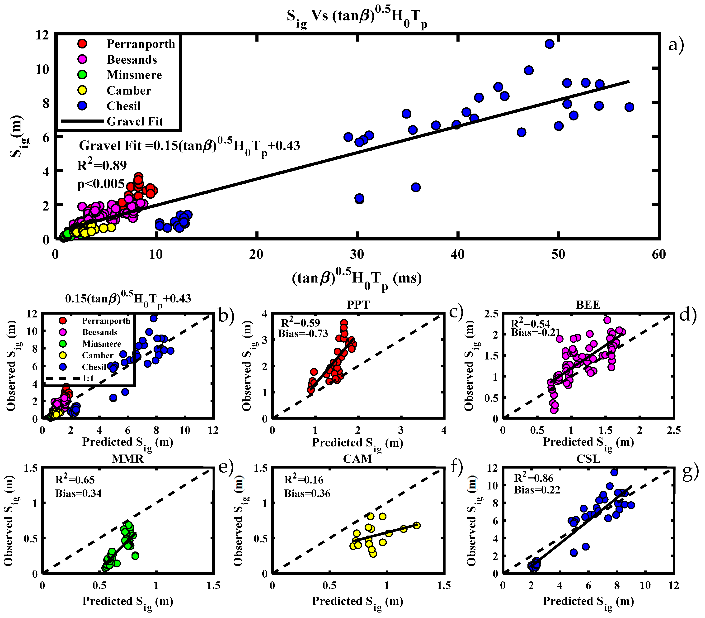
3.4.2. Poate—Gravel Beaches

While no gravel specific predictors of S_ig exist, Reference [17] (P2016) developed a predictor of runup elevation using a range of data from four gravel beaches and synthetic data from the gravel specific numerical model, X-beach-G, finding that inclusion of a beach slope term yielded the most accurate predictor (R2% = C (tan β)^0.5H₀T_p, where C is a constant). Given that P2016 was designed to predict runup, as opposed to S_ig, the constant suggested by Reference [17] (C = 0.33) is not applicable to the prediction of S_ig. Instead, using the terms in P2016, a value of C was derived here by applying a linear best fit to the combined set of data from the gravel sites (Beesands and Chesil) (Figure 8a), yielding a gravel specific predictor of S_ig, as shown in Equation (5).

S_ig = 0.15(tan β)^0.5 H₀T_p + 0.43.

(5)

Given that in S2006 wave height is square-rooted, a greater emphasis is placed on H₀ in Equation (5). This increased emphasis on H₀, combined with the introduction of tan β, implies that wave height and beach slope play a more critical role in the control of S_ig on gravel beaches than sandy ones.

On the compound/mixed sites, S_ig was reasonably well predicted at Minsmere, although Figure 8e reveals a small but systematic over-prediction of S_ig, yielding a bias of 0.34 m, while Camber showed no significant relationship between S_ig and Equation (5). Of the significantly related sites (all except Camber), S_ig was least well predicted by Equation (5) at Perranporth (Figure 8a–c), with a large negative bias (−0.73) representing an under-prediction of S_ig. The enhanced infragravity levels at Perranporth may result from the efficient transfer of energy to lower frequencies across the wide, dissipative surf zone.

3.4.3. Deepwater Wave Power

S2006 and Equation (5) were shown to skillfully predict S_ig at a specific type of beach over a specific range of conditions. In order to examine whether S_ig could be predicted with any skill during extreme waves at contrasting sites, the relationship with deep water wave power was tested. Wave power is frequently used in the parameterization of storm hydrodynamics [29,30,31]. Removing the constants from the deep water waver power equation yields P∝H₀²T, a useful parameterization previously applied to infragravity waves on a dissipative sandy beach by Inch et al. (2017). S_ig was regressed against H₀²T for the combined dataset of all five sites (Figure 9a), deriving a linear equation for predicting S_ig.

S_ig = 0.02(H₀²T) + 0.42,

(6)

Equation (6) skillfully predicted S_ig at Beesands, Perranporth, and Chesil with small biases of −0.23, 0.30, and 0.38 m, respectively (Figure 9d,c,g, respectively), suggesting that infragravity swash height is proportional to deep water wave power in extreme wave conditions at these three contrasting sites, all of which are susceptible to infragravity dominance at the shoreline (Figure 6). Equation 6 was a less suitable predictor of S_ig at the mixed sand and gravel sites, yielding larger biases at Minsmere (0.49 m) (Figure 9e) and showing no significant relationship with S_ig at Camber (p = 0.248) (Figure 9f).

3.4.4. Comparison of Parameterizations

Section 3.4 thus far demonstrated that the relationship between wave and beach statistics and S_ig varies between sites. The predictive skill of S2006, and Equations (5) and (6) at the five contrasting sites is compared in

Table 5. Comparison of relationships between observed S_ig and S_ig predicted by S2006, and Equations (5) and (6).

Equation	Site	R2	Bias	p-Value
S2006 Sig = 0.06 (H0L0)0.5
	Perranporth	0.61	−0.33	<0.005
	Beesands	0.36	−0.57	<0.005
	Minsmere	0.63	0.27	<0.005
	Camber	0.12	0.32	0.014
	Chesil	0.60	−3.0	<0.005
Equation (5) Sig = 0.15(tan β)0.5H0Tp + 0.43
	Perranporth	0.59	−0.73	<0.005
	Beesands	0.54	−0.21	<0.005
	Minsmere	0.65	0.34	<0.005
	Camber	0.16	0.36	0.123
	Chesil	0.86	0.22	<0.005
Equation (6) Sig = 0.02(H02T) + 0.42
	Perranporth	0.70	0.3	<0.005
	Beesands	0.52	−0.23	<0.005
	Minsmere	0.65	0.49	<0.005
	Camber	0.09	0.72	0.248
	Chesil	0.81	0.38	<0.005

.

S_ig at Perranporth was accurately predicted by both S2006 and Equation (6), with marginally higher R² for the latter. At Beesands, both Equations (5) and (6) were strong predictors of S_ig. The low levels of S_ig observed at Minsmere were well predicted by all three equations, with S2006 yielding the lowest biases. S_ig at Camber was generally low and showed no relationship with any of the three equations. At Chesil, S_ig was well predicted by Equations (5) and (6).

Given that Equation (5) was derived from data collected at Beesands and Chesil, a more skillful predictor is Equation (6). Of the sites susceptible to IG dominance (Perranporth, Beesands, and Chesil), S_ig can be accurately predicted by Equation (6), under high-energy conditions, demonstrating that large offshore wave powers associated with big swell waves are the main driver of large infragravity energy in the swash across these widely varying beach types.

4. Discussion

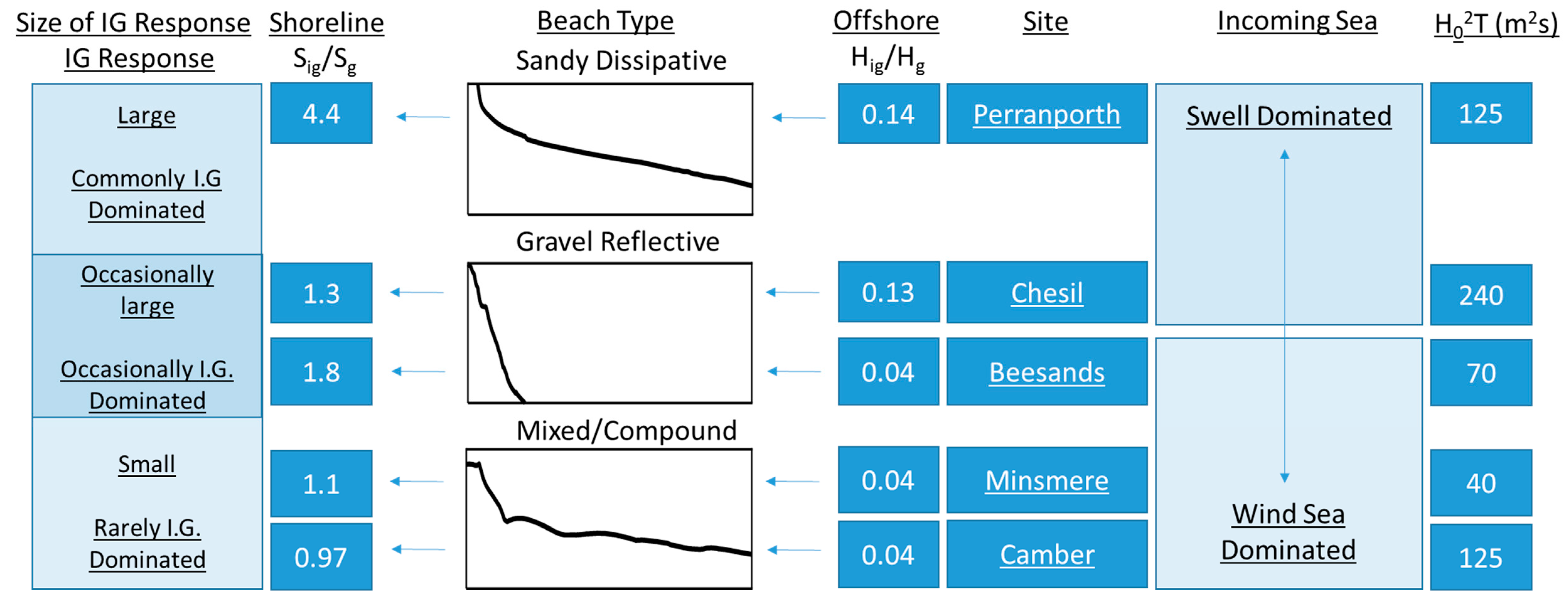
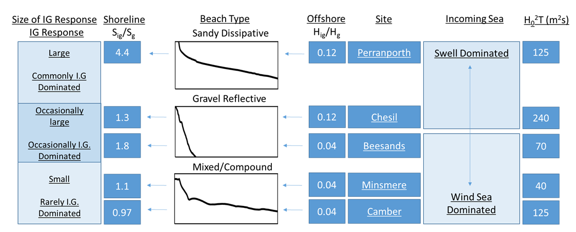
Conceptual Diagram—When and Where Are Infragravity Waves Important at the Shoreline?

Table 6. Representative infragravity heights and dominance, at the shoreline and offshore, during the times of high incident wave energy, as presented in Figure 4.

	Shoreline		Offshore
Site	Sig (m)	Sig/Sg	Hsig (m)	Hig/Hg
PPT	2.5	4.4	0.42	0.14
CSL	6.4	1.3	0.73	0.13
BEE	1.9	1.8	0.10	0.04
MMR	0.7	1.1	0.09	0.04
CAM	0.8	0.97	0.16	0.04

and Figure 10 summarize the contrasting behavior of energy in the gravity and infragravity band from offshore to the shoreline, under extreme conditions, on three distinct morphologies (sand, gravel, and compound/mixed). Taking the data runs presented in Figure 4 as examples of high-energy/extreme conditions, from right to left, the diagram displays the following for each of the five study sites: incoming wave power and sea state, ratio of infragravity to gravity offshore, representative profile, resultant infragravity to gravity ratio at the shoreline, and relative size and dominance attributed to each of the three distinct morphologies.

Despite contrasting values of incoming wave power, the ratio H_ig/H_g was the same (0.12) at both the swell-dominated sites (Perranporth and Chesil). This value of H_ig/H_g was the largest observed across all sites.

Despite a larger increase in infragravity height between the offshore (H_ig) and the shoreline (S_ig) on gravel beaches than sand (Table 6), the ratio of S_ig/S_g was largest on the sandy site (Perranporth) (4.4), over three times as large as Chesil and twice as large as Beesands. This demonstrated that a lack of short wave dissipation on steep gravel morphology, compared to the sandy one, limited infragravity dominance at the shoreline. Of the two gravel sites, the relatively steeper waves and lower beach slope at Beesands compared to Chesil resulted in more efficient short wave dissipation and an increased ratio of S_ig/S_g, as observed in Table 6 and Figure 10.

Despite the range in values of H²T, the ratio of H_ig/H_g was comparable at Beesands, Minsmere, and Camber (~0.04). These are all fetch-limited sites, dominated by local wind-waves. This, along with the lower values of H_ig at Beesands, Camber, and Minsmere compared to Perranporth and Chesil, demonstrated a clear separation between swell- and wind-wave-dominated sites (Figure 10).

For the wind-wave-dominated sites, a contrasting response in both the ratio and IG height between offshore and the shoreline was observed between the gravel and mixed/compound morphology. The gravel profile was susceptible to IG dominance with a ratio of up to 1.8. The compound sites were either never or rarely IG-dominated.

5. Summary and Conclusions

Significant swash height in the gravity (S_g) and infragravity bands (S_ig) was obtained from video runup data, under an unprecedented range of wave and beach conditions. Observations included extreme waves, in excess of the 95th percentile at five contrasting sites, ranging from both wind-wave- and swell-dominated gravel beaches, through fetch-limited mixed sand and gravel, to a swell-dominated, low-sloping sandy beach.

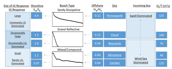
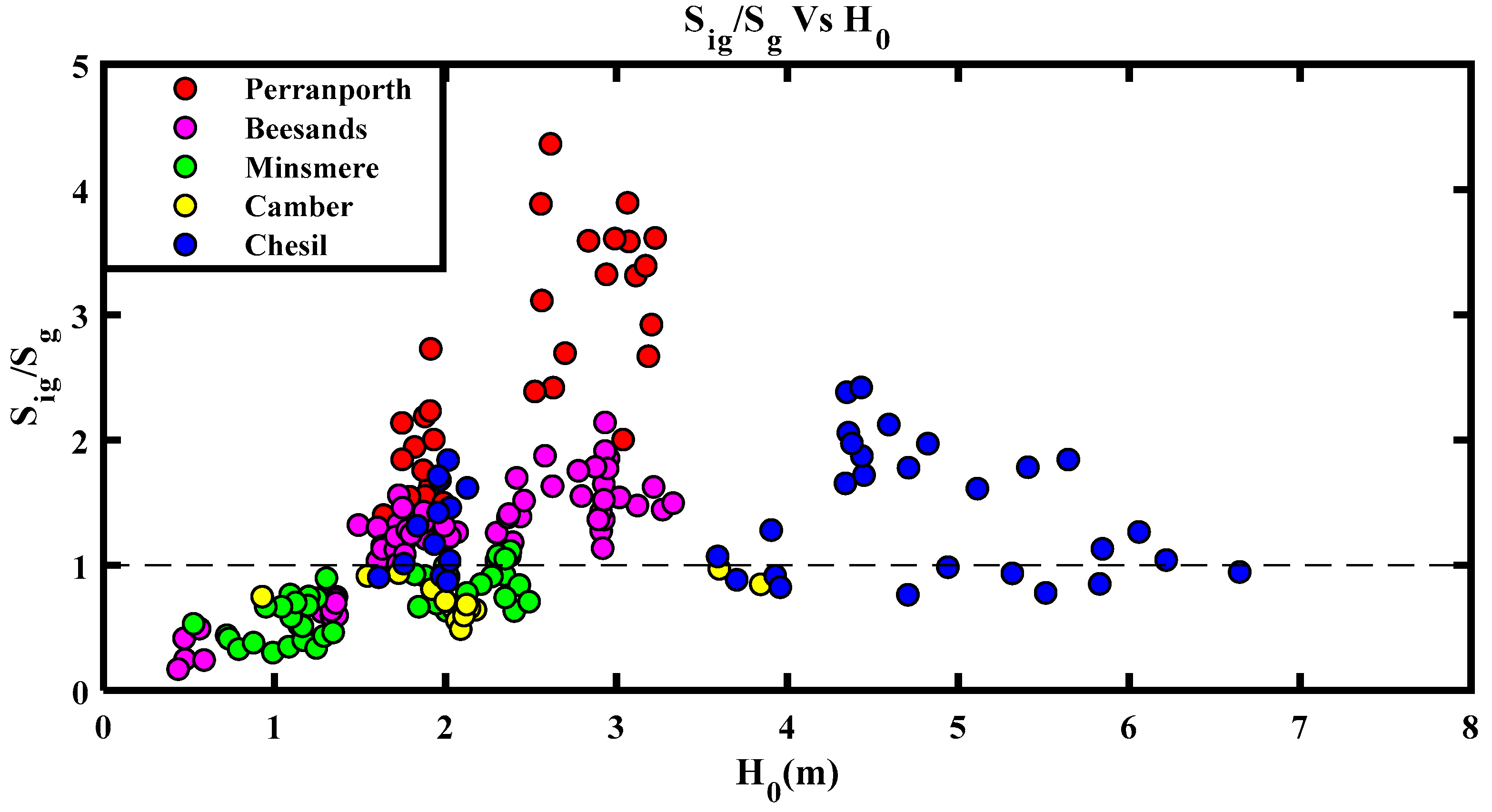
• Infragravity waves were observed in the swash at all sites, becoming important when H₀ exceeded approximately 1.3 m. For a given wave height, infragravity waves in the swash were enhanced on gravel and sandy beaches, but suppressed on mixed/compound beaches.
• Infragravity waves were observed to become most dominant in the swash on the low sloping sandy beach, where S_ig/S_g exceeded 4. They occasionally dominated the gravel beaches, but to a lesser extent (<1.8), and rarely or never dominated the mixed/compound sites (<1.1). This was attributed to differences in short wave dissipation patterns resulting from contrasting morphology and wave steepness.
• A previously published empirical relationship [10], S_ig = 0.06 (H₀L₀)^0.5, developed on sandy beaches, predicted S_ig well on the sandy beach and the mixed sand and gravel beach, over a comparable range of conditions to those in which it was developed. Stockdon was shown to under-predict S_ig for higher-energy conditions and for data collected on gravel beaches, suggesting S_ig was enhanced under these conditions.
• A new gravel specific predictor of S_ig was proposed, by linearly fitting observations of S_ig from two separate field deployments to terms from Poate’s gravel runup equation, (tan β)^1/2H₀T_p. This was seen to underestimate values of S_ig on the sandy beach.
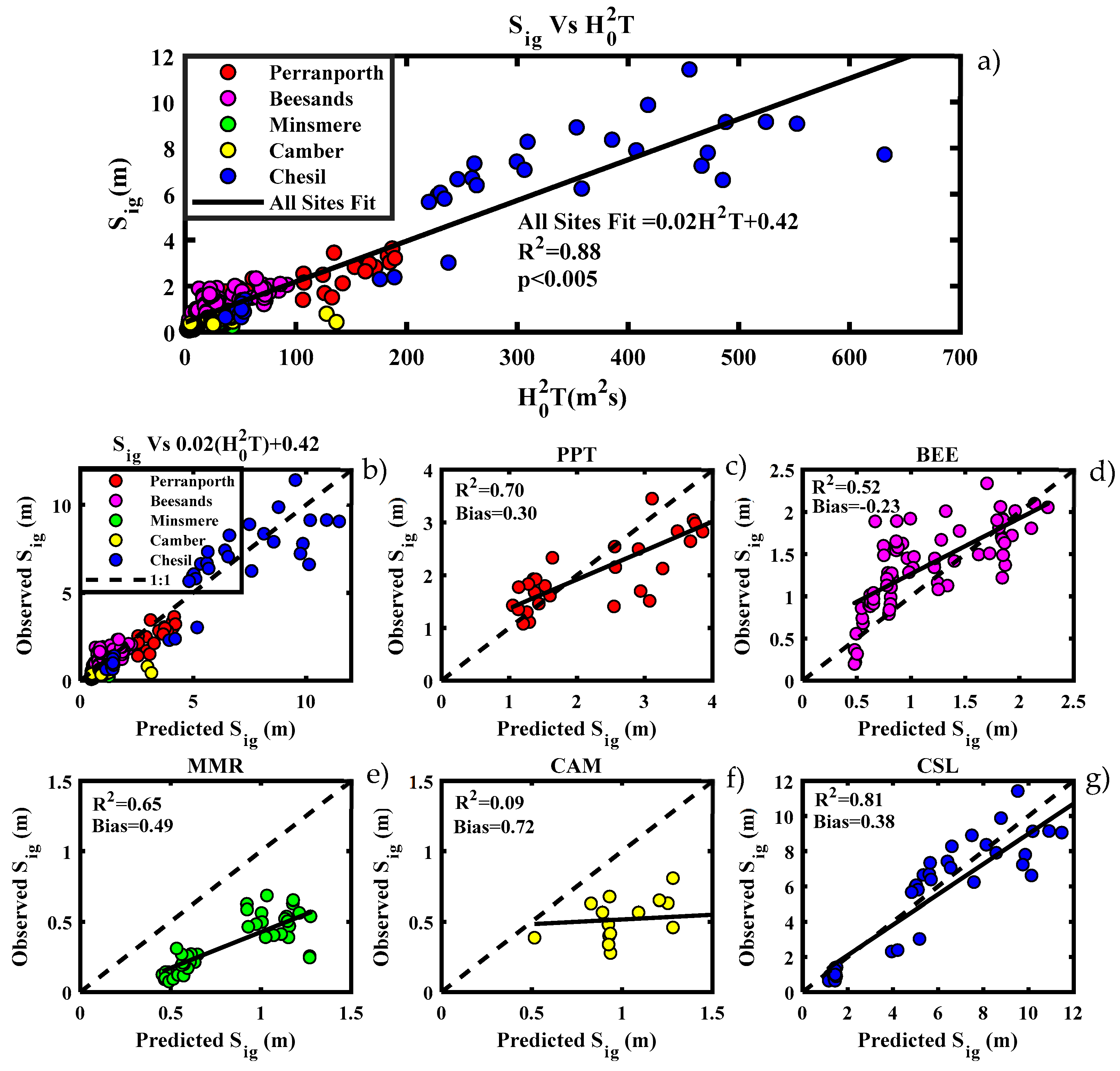
• H₀²T, proportional to offshore wave power, was a good predictor of S_ig at the sites where IG could become dominant, yielding the equation S_ig = 0.02(H₀²T) + 0.42, valid for high-energy conditions.
• The relationship between S_ig and H₀²T across a diverse range of sites implied that, under extreme wave conditions, wave height and period became more important than local morphology as a control on infragravity in the swash. Conversely, at sites where IG rarely dominated, infragravity swash height remained small at the shoreline regardless of offshore conditions. This highlights the importance of collecting data over the unique range of heights and periods present here.

A conceptual model was presented summarizing the contrasting development of infragravity energy at the shoreline on three distinct morphologies (sand, gravel, and compound/mixed). This showed that increases in IG height between offshore and the shoreline were greatest on gravel beaches, moderate on sandy beaches, and smallest on compound/mixed beaches. Infragravity became more dominant in the swash on sand rather than gravel sites. This resulted in the swash being commonly IG-dominated on low-sloping sandy beaches, occasionally IG-dominated on gravel beaches, and rarely IG-dominated on compound/mixed beaches.

References

1. McCall, R.T.; Van Thiel de Vries, J.S.M.; Plant, N.G.; Van Dongeren, A.R.; Roelvink, J.A.; Thompson, D.M.; Reniers, A.J.H.M. Two-dimensional time dependent hurricane overwash and erosion modeling at Santa Rosa Island. Coast. Eng. 2010, 57, 668–683. [Google Scholar] [CrossRef]
2. Roelvink, D.; Reniers, A.; van Dongeren, A.; van Thiel de Vries, J.; McCall, R.; Lescinski, J. Modelling storm impacts on beaches, dunes and barrier islands. Coast. Eng. 2009, 56, 1133–1152. [Google Scholar] [CrossRef]
3. Russell, P.E. Mechanisms for beach erosion during storms. Cont. Shelf Res. 1993, 13, 1243–1265. [Google Scholar] [CrossRef]
4. Raubenheimer, B.; Guza, R.T. Observations and predictions of run-up. J. Geophys. Res. Ocean. 1996, 101, 25575–25587. [Google Scholar] [CrossRef]
5. Oltman-shay, J. Infragravity Energy and its Implications in Nearshore Sediment Transport and Sandbar Dynamics; Forgotten Books: London, UK, 1989. [Google Scholar]
6. Senechal, N.; Coco, G.; Bryan, K.R.; Holman, R.A. Wave runup during extreme storm conditions. J. Geophys. Res. Ocean. 2011, 116, 1–13. [Google Scholar] [CrossRef]
7. Fiedler, J.W.; Brodie, K.L.; McNinch, J.E.; Guza, R.T. Observations of runup and energy flux on a low-slope beach with high-energy, long-period ocean swell. Geophys. Res. Lett. 2015, 42, 9933–9941. [Google Scholar] [CrossRef]
8. Inch, K.; Davidson, M.; Masselink, G.; Russell, P. Observations of nearshore infragravity wave dynamics under high energy swell and wind-wave conditions. Cont. Shelf Res. 2017, 138, 19–31. [Google Scholar] [CrossRef]
9. Bertin, X.; de Bakker, A.; van Dongeren, A.; Coco, G.; Andrée, G.; Ardhuinf, F.; Bonneton, P.; Bouchette, F.; Castelle, B.; Crawford, W.; et al. Infragravity wave: From driving mechanisms to impacts. Earth Sci. Rev. 2018, 1–70. [Google Scholar] [CrossRef]
10. Stockdon, H.F.; Holman, R.A.; Howd, P.A.; Sallenger, A.H. Empirical parameterization of setup, swash, and runup. Coast. Eng. 2006, 53, 573–588. [Google Scholar] [CrossRef]
11. Masselink, G.; Puleo, J.A. Swash-zone morphodynamics. Cont. Shelf Res. 2006, 26, 661–680. [Google Scholar] [CrossRef]
12. Passarella, M.; Goldstein, E.B.; De Muro, S.; Coco, G. The use of genetic programming to develop a predictor of swash excursion on sandy beaches. Nat. Hazards Earth Syst. Sci. 2018, 18, 599–611. [Google Scholar] [CrossRef]
13. Gomes da Silva, P.; Medina, R.; González, M.; Garnier, R. Infragravity swash parameterization on beaches: The role of the profile shape and the morphodynamic beach state. Coast. Eng. 2018, 136, 41–55. [Google Scholar] [CrossRef]
14. Guedes, R.M.C.; Bryan, K.R.; Coco, G.; Holman, R.A. The effects of tides on swash statistics on an intermediate beach. J. Geophys. Res. Ocean. 2011, 116, 1–13. [Google Scholar] [CrossRef]
15. Guedes, R.M.C.; Bryan, K.R.; Coco, G. Observations of wave energy fluxes and swash motions on a low-sloping, dissipative beach. J. Geophys. Res. Ocean. 2013, 118, 3651–3669. [Google Scholar] [CrossRef]
16. Hunt, I.A. Design of Seawalls and Breakwaters. J. Waterw. Harb. Div. 1959, 85, 123–152. [Google Scholar]
17. Poate, T.G.; McCall, R.T.; Masselink, G. A new parameterisation for runup on gravel beaches. Coast. Eng. 2016, 117, 176–190. [Google Scholar] [CrossRef]
18. Guza, R.T.; Thornton, E.B. Swash oscillations on a natural beach. J. Geophys. Res. 1982, 87, 483–491. [Google Scholar] [CrossRef]
19. Ruessink, B.G.; Kleinhans, M.G.; van den Beukel, P.G.L. Observations of swash under highly dissipative conditions. J. Geophys. Res. 1998, 103, 3111–3118. [Google Scholar] [CrossRef]
20. Ruggiero, P.; Holman, R.A.; Beach, R.A. Wave run-up on a high-energy dissipative beach. J. Geophys. Res. C Ocean. 2004, 109. [Google Scholar] [CrossRef]
21. Jennings, R.; Shulmeister, J. A field based classification scheme for gravel beaches. Mar. Geol. 2002, 186, 211–228. [Google Scholar] [CrossRef]
22. Harley, M. Coastal Storm Definition. In Coastal Storms: Processes and Impacts; John Wiley & Sons: Hoboken, NJ, USA, 2017; pp. 1–21. [Google Scholar]
23. Battjes, J.A. Surf Similarity. In Proceedings of the 14th International Conference on Coastal Engineering, Copenhagen, Denmark, 24–28 June 1974; pp. 466–480. [Google Scholar]
24. Almeida, L.P.; Masselink, G.; Russell, P.; Davidson, M.; Poate, T.; McCall, R.; Blenkinsopp, C.; Turner, I. Observations of the swash zone on a gravel beach during a storm using a laser-scanner (Lidar). J. Coast. Res. 2013, 65, 636–641. [Google Scholar] [CrossRef]
25. Almeida, L.P.; Masselink, G.; Russell, P.E.; Davidson, M.A. Observations of gravel beach dynamics during high energy wave conditions using a laser scanner. Geomorphology 2015, 228, 15–27. [Google Scholar] [CrossRef]
26. Earlie, C.S.; Young, A.P.; Masselink, G.; Russell, P.E. Coastal cliff ground motions and response to extreme storm waves. Geophys. Res. Lett. 2015, 847–854. [Google Scholar] [CrossRef]
27. Holland, K.T.; Holman, R.A.; Lippmann, T.C.; Stanley, J.; Plant, N. Practical Use of Video Imagery in Nearshore Oceanographic Field Studies. IEEE J. Ocean. Eng. 1997, 22, 81–92. [Google Scholar] [CrossRef]
28. Austin, M.J.; Masselink, G. Observations of morphological change and sediment transport on a steep gravel beach. Mar. Geol. 2006, 229, 59–77. [Google Scholar] [CrossRef]
29. Scott, T.; Masselink, G.; Russell, P. Morphodynamic characteristics and classi fi cation of beaches in England and Wales. Mar. Geol. 2011, 286, 1–20. [Google Scholar] [CrossRef]
30. Burvingt, O.; Masselink, G.; Russell, P.; Scott, T. Classification of beach response to extreme storms. Geomorphology 2017, 295, 722–737. [Google Scholar] [CrossRef]
31. Wiggins, M.; Scott, T.; Masselink, G.; Russell, P.; McCarroll, R.J. Coastal embayment rotation: Response to extreme events and climate control, using full embayment surveys. Geomorphology 2019, 327, 385–403. [Google Scholar] [CrossRef]
Figure 1. Location of sites previously studied, listed in Table 1, showing variation between ocean-facing and fetch-limited sites: (a); world map; (b) United States of America (USA); (c) Western Europe; (d) New Zealand.
Jmse 07 00139 g001
Figure 2. Location (top left corner), photographs (left), and representative profiles (to the right of the photographs) of (a) Perranporth (PPT), (b) Beesands (BEE), (c) Chesil (CSL), (d) Camber (CAM), and (e) Minsmere (MMR). Dashed black lines on the profiles represent mean high and low water spring tidal elevation. The Chesil photograph (c) is licensed under the Creative Commons Attribution-Share Alike 3.0 Unported license (https://creativecommons.org/licenses/by-sa/3.0/deed.en).
Jmse 07 00139 g002
Figure 3. Video processing technique: example from 26 February 2018 from 3:30–3:50 p.m. at Beesands. (a) Analyzed profile to be extracted (black line); (b) pixel stack with shoreline detected and time series of horizontal swash (black line); (c) vertical swash time series relative to still water level (SWL).
Jmse 07 00139 g003
Figure 4. Frequency smoothed wave spectra showing examples of simultaneous power spectral densities (PSD) offshore and at the shoreline. (a,c,e,g,i): Waves measured at local wave buoys (solid black line). (b,d,f,h,j): Vertical swash at the shoreline (solid black line). Both: 95% confidence interval (dashed grey line). Infragravity and gravity bands are separated by a vertical black line at 0.05 Hz. a + b = Perranporth (PPT), c + d = Chesil (CSL), e + f Beesands = (BEE), g + h = Camber (CAM), i + j = Minsmere (MMR).
Jmse 07 00139 g004
Figure 5. Significant swash height against offshore significant wave height (H0). Left panel shows the incident gravity band (Sg). Right panel shows the infragravity band (Sig), where the black line represents the linear best fit for all sites.
Jmse 07 00139 g005
Figure 6. Sig/Sg against H0. Transition from Sg- (below) to Sig-dominated (above) (horizontal dashed line).
Jmse 07 00139 g006
Figure 7. (a) Significant infragravity swash height Sig against (H0L0)0.5 after Stockdon et al. (2006). Linear best fit for Stockdon 2006 data (solid orange line), limited to the original range of (H0L0)0.5. (b) Comparison of Sig heights observed and those predicted by S2006 at all sites. (cg) As above but for individual sites.
Jmse 07 00139 g007
Figure 8. (a) Significant infragravity swash height Sig against (tan β)0.5H0Tp. Linear best fit for Beesands and Chesil (Equation (5)), black line. (b) Comparison of Sig heights observed and those predicted by Equation (5) at all sites. (cg) As above, but for individual sites. Equation (5) has a y-axis intercept (c) of 0.43 resulting from the linear fit being extended beyond the lowest observed values of 0.15(tan β)0.5H0Tp. Given the positive intercept, Equation (5) should not be extended beyond the range of observed values of (tan β)0.5H0Tp and is, therefore, only applicable for values above 0.8 ms.
Jmse 07 00139 g008
Figure 9. (a) Significant infragravity swash height Sig against H02T. Linear best fit for all sites (Equation (6)), black line. (b) Comparison of Sig heights observed and those predicted by Equation (6) at all sites. (cg) As above, but for individual sites. Equation (6) is only valid for high-energy conditions.
Jmse 07 00139 g009
Figure 10. Conceptual diagram summarizing the contrasting development of infragravity energy at the shoreline on three distinct morphologies: sand, gravel, and mixed/compound. The numerical values used in the diagram are taken from Figure 4 and are representative of high-energy conditions at each site.
Jmse 07 00139 g010