Two-Dimensional Numerical Study of Seabed Response around a Buried Pipeline under Wave and Current Loading

Abstract

The evaluation of the wave-induced seabed response around a buried pipeline has been widely studied. However, the analysis of seabed response around marine structures under the wave and current loadings are still limited. In this paper, an integrated numerical model is proposed to examine the wave and current-induced pore pressure generation, for instance, oscillatory and residual pore pressure, around a buried pipeline. The present wave–current model is based on the Reynolds-Averaged Navier–Stokes (RANS) equation with $k$-$\epsilon$ turbulence while Biot’s equation is adopted to govern the seabed model. Based on this numerical model, it is found that wave characteristics (i.e., wave period), current velocity and seabed characteristics such as soil permeability, relative density, and shear modulus have a significant effect on the generation of pore pressure around the buried pipeline.

1. Introduction

Submarine pipelines are frequently used in the transportation of hydrocarbons such as oil and natural gas from offshore platforms to onshore terminals and in the disposal of industrial and municipal waste in offshore engineering. Since these submarine pipelines play such an important role, it has become one of the significant concern in marine and geotechnical engineering. Generally, submarine pipelines are buried into the seabed or within a trench. In the ocean environment, as waves propagate over the ocean floor, they generate dynamic pressure fluctuations, which will further induce excess pore pressure and reduce effective stress within the seabed soil. As the excess pore pressure increases, the soil particles loses its strength and part of the seabed becomes unstable. In most of the cases, seabed instability is the primary cause that leads to marine structure failure. Therefore, it is essential for offshore engineers to evaluate the wave-induced seabed response.

To date, numerous studies on wave-induced seabed response with marine structures such as breakwaters [1], monopiles [2] and pipelines [3] or without marine structures [4,5] had already been carried out. Based on laboratory experiments and field studies [6], the wave-induced pore pressure classifies into two mechanisms, which are oscillatory and residual mechanisms, as shown in Figure 1. Oscillatory pore pressure generation is caused by the amplitude damping and phase lag in pore pressure whereas residual pore pressure generation is the build-up excess pore pressure, which caused by the contraction of soil resulted from cyclic loading [7].

In the real ocean environment, water waves and current flows exist simultaneously. Hence, in addition to wave loadings, current loadings should also be taken into consideration. Recently, numerous researchers [8,9,10,11,12] have conducted studies to understand the interaction between wave, current, and seabed. In general, to understand the phenomenon of wave–current–seabed interaction (WCSI) and wave–current–seabed-structure interaction (WCSSI), three common approaches are widely adopted, which are the analytical solution, laboratory experiments, and numerical methods. For the study of WCSI, Zhang et al. [13] and Liao et al. [14] developed an analytical approximation to calculate the soil response of a porous seabed under the combination of wave and current loading. In many cases, to simplify the problems, seabed condition is assumed to be isotropic. In Zhou’s [15] research, the soil response in anisotropic seabed with a buried marine pipeline was calculated using the analytical method. In the analytical approach, most researchers utilized the third approximation wave–current interactions as the governing equation to determine the dynamic pressure from the wave model, which eventually used as the boundary condition for the porous seabed analysis in the seabed model.

Besides analytical method, laboratory experiments have also been reported in the literature. Liu et al. [16] conducted a series of experimental studies using a one-dimensional cylinder. The purpose of a one-dimensional cylinder experiment is to determine the wave-induced oscillatory soil response and to obtain the vertical profile of the pore pressure distribution. Two or three-dimensional wave flume tank experiments [17,18] and centrifuge modeling [19,20] were conducted in the laboratory to study WCSSI phenomenon and the stability of a pipeline. There are advantages and limitations to one-dimensional cylinder experiments and two-dimensional wave flume tank experiments or centrifuge experiments. For a one-dimensional cylinder experiment, many points can be measured due to their thick soil layers, but only oscillatory pore pressure and the vertical pore pressure distribution is obtained, whereas for a two-dimensional experiment, the accumulation of build-up excess pore pressure can be analyzed, but fewer surface points are measured due to the shallow soil layers. Recently, Yang et al. [21] conducted a flume experiment using a new method of the grey value of water’s image to study the initial movement of mud particles due to current loading.

As the problem becomes more complicated to be solved by analytical solution and laboratory experiments, numerical methods are usually performed. Several researchers [11] had conducted numerical simulations to study the wave–current induced seabed response without any presence of marine structures. With the inclusion of marine structures such as pipelines in the seabed, the soil responses vary under wave and current loading. Zhao et al. conducted a two-dimensional model to study the influences of pore pressure accumulations around the vicinity of a fully buried pipeline in the seabed [22] and protected in trench layer with partial backfills [23]. Zhou et al. [24] simulated the pore pressures, effective stresses and liquefaction potential around a buried in a poroelastic seabed subjected to cnoidal wave loading. In both Zhao’s and Zhou’s studies, only wave loading takes into consideration. Recently, Duan et al. performed a two-dimensional [25] and three-dimensional [26] numerical simulation to study the wave–current induced soil liquefaction around the buried pipeline. However, in their research, only the oscillatory soil response under a wave and current loading have been determined. The wave–current induced oscillatory soil response is influenced by the current characteristics (following or opposing currents), wave characteristics (i.e., wave height, wave period and water depth) and soil properties (i.e., backfill thickness, permeability, and degree of saturation). Relevant research on wave–current–seabed-structure interaction is still limited. Therefore, more studies still needed to be conducted to provide a better understanding of this phenomenon.

In the present study, the objective is to develop a numerical model to analyze the pore pressure accumulation around the vicinity of a fully buried pipeline when the seabed is subjected to wave and current loadings. This numerical analysis consists of two submodels, which are the wave–current model and the seabed model. In the wave–current model, RANS equation with $k$-$\epsilon$ turbulence governs the wave motion and current flow, whereas in the seabed model, Biot’s quasi-static equations are employed to calculate soil response such as soil displacements, oscillatory pore pressure, residual pore pressure and the effective stress within the seabed. The influence of wave, current, and seabed characteristics such as current velocities, wave period, shear modulus, permeability, and relative density on the soil responses are presented and discussed in the later sections.

2. Methods

This numerical model is made up of two submodels: wave–current model and seabed model with a buried pipeline. These two submodels are integrated with one-way coupling method. For a one-way coupling method of fluid-seabed interactions [27], the wave pressure computed in the wave solver is introduced into the seabed solver as a boundary condition to solve for the seabed response. Figure 2 illustrates a wave–current–seabed-structure interaction (WCSSI), where x and z represents the Cartesian coordinates system, h is the seabed thickness, d is the water depth, l is the length of the computational domain, e represents the embedment depth of pipeline (i.e., the distance from the surface of the seabed to the center of the pipeline) and u is the initial current velocity. In this study, the length of the computational domain (l) is set to be three times the wavelength to ignore the influence of lateral boundaries.

2.1. Wave–Current Model

The wave and current interaction model is based on the Reynolds-Averaged Navier–Stokes equation to simulate the flow motion. For the incompressible fluids, the mass conservation equation and the momentum conservation equation can be expressed as below:

$$\frac{\partial u_i}{\partial x_i}=0,$$

(1)

$$\frac{\partial \langle u_i\rangle }{\partial t}+\frac{\partial \langle u_i\rangle \langle u_j\rangle }{\partial x_j}=-\frac{1}{{\rho }_f}\frac{\partial \langle p\rangle }{\partial x_i}+g_i+\frac{1}{{\rho }_f}\frac{\partial }{\partial x_j}\left[\mu \left(\frac{\partial \langle u_i\rangle }{\partial x_j}+\frac{\partial \langle u_j\rangle }{\partial x_i}\right)\right]-\frac{\partial \langle u_i^{\prime }{u}_j^{\prime }\rangle }{\partial x_j},$$

(2)

where $x_i$ represents the Cartesian coordinate, $({)}_i$ and $({)}_j$ represent the index tensor notion, $\langle u_i\rangle$ is the ensemble mean velocity (m/s), $\langle p\rangle$ is the fluid pressure (Pa), ${\rho }_f$ is the fluid density (kg/m³), $t$ is the time, $g$ is the acceleration (m/s²), $\mu$ is the dynamic viscosity (Pa·s), and $-{\rho }_f\langle u_i^{\prime }{u}_j^{\prime }\rangle$ is the Reynolds stress tensor. By applying the eddy-viscosity assumptions, Reynold stress term can be expressed as:

$$-{\rho }_f\langle u_i^{\prime }{u}_j^{\prime }\rangle =\mu \left[\frac{\partial \langle u_i\rangle }{\partial x_j}+\frac{\partial \langle u_j\rangle }{\partial x_i}\right]-\frac{2}{3}{\rho }_f{\delta }_{ij}k,$$

(3)

where ${\mu }_t$ is the turbulence viscosity (Pa·s), $k$ is the turbulence kinetic energy (TKE, m²/s²), and ${\delta }_{ij}$ is the Kronecker delta. By substituting Equation (3) into Equation (2), the following equation can be obtained:

$$\frac{\partial {\rho }_f\langle u_i\rangle }{\partial t}+\frac{\partial {\rho }_f\langle u_i\rangle \langle u_j\rangle }{\partial x_j}=-\frac{\partial }{\partial x_i}\left[\langle p\rangle +\frac{2}{3}{\rho }_{f}k\right]+{\rho }_f{g}_i+\frac{\partial }{\partial x_j}\left[{\mu }_{eff}\left(\frac{\partial \langle u_i\rangle }{\partial x_j}+\frac{\partial \langle u_j\rangle }{\partial x_i}\right)\right],$$

(4)

where ${\mu }_{eff}$ = $\mu +{\mu }_t$, which is the total effective viscosity (Pa·s).

For the prediction of a fully turbulent flow, the standard $k$-$\epsilon$ turbulence model [28] based on model transport equations for the turbulence kinetic energy and its rate of dissipation can be expressed as follows:

$$\frac{\partial {\rho }_{f}k}{\partial t}+\frac{\partial {\rho }_f\langle u_j\rangle k}{\partial x_j}=-\frac{\partial }{\partial x_j}\left[\left(\mu +\frac{{\mu }_t}{{\sigma }_k}\right)\frac{\partial k}{\partial x_j}\right]+{\rho }_f{{}^{\prime }\mathrm{P}}_k-{\rho }_f\epsilon ,$$

(5)

$$\frac{\partial {\rho }_f\epsilon }{\partial t}+\frac{\partial {\rho }_f\langle u_j\rangle \epsilon }{\partial x_j}=-\frac{\partial }{\partial x_j}\left[\left(\mu +\frac{{\mu }_t}{{\sigma }_{\epsilon }}\right)\frac{\partial \epsilon }{\partial x_j}\right]+\frac{\epsilon }{k}\left(C_{\epsilon 1}{\rho }_f{{}^{\prime }\mathrm{P}}_k-C_{\epsilon 2}{\rho }_f\epsilon \right),$$

(6)

where ${\mu }_t={\rho }_f{C}_{\mu }\frac{k^2}{\epsilon }$, $k$ is the turbulence kinetic energy (m²/s²), $\epsilon$ is the turbulence dissipation rate, $C_{\mu },{\sigma }_k, {\sigma }_{\epsilon }, C_{\epsilon 1},$ and $C_{\epsilon 2}$ are the empirical coefficients determined from experiments. The empirical coefficients used in this study are based on previous studies [29]:

$$C_{\mu }=0.09C_{\epsilon 1}=1.44C_{\epsilon 2}=1.92{\sigma }_k=1.00{\sigma }_{\epsilon }=1.30$$

2.2. Seabed Model

As mentioned earlier, pore pressure generation classifies into two mechanisms: oscillatory pore pressure and residual pore pressure. The pore pressure generation can be expressed as follows:

$$u=u_e+u_p$$

(7)

where $u$ represents the wave and current-induced excess pore pressure at a specific point, $u_e$ is the oscillatory component whereas $u_p$ is the residual component that is further expressed as $u_p=\frac{1}{T}{{\displaystyle \int }}_0^{T}udt$ where T denotes the wave period.

2.2.1. Oscillatory Soil Response

In this study, the seabed model is considered to be porous and hydraulically permeable. The soil skeleton and pore fluid are assumed to be compressible and obey the Hooke’s Law. Therefore, Biot’s theory [30] is utilized to govern the soil response. The mass conservation and force equilibrium equation can be written as follows:

$${\nabla }^2{u}_e-\frac{{\gamma }_w{n}_s{\beta }_s}{k_s}\frac{\partial u_e}{\partial t}=\frac{{\gamma }_w}{k_s}\frac{\partial {\epsilon }_s}{\partial t}$$

(8)

$$G{\nabla }^2{u}_s+\frac{G}{\left(1-2\nu \right)}\frac{\partial {\epsilon }_s}{\partial x}=-\frac{\partial u_e}{\partial x},$$

(9)

$$G{\nabla }^2{w}_s+\frac{G}{\left(1-2\nu \right)}\frac{\partial {\epsilon }_s}{\partial z}=-\frac{\partial u_e}{\partial z},$$

(10)

where ${\nabla }^2=\left(\frac{{\partial }^2}{\partial x^2} \frac{{\partial }^2}{\partial z^2}\right)$ represents the Laplace operator,${\gamma }_w$ is the unit weight of water (N/m³), $n_s$ is the soil porosity, $k_s$ is the soil permeability (m/s), $G$ denotes the shear modulus of the seabed soil (N/m²), $\nu$ is the Poisson’s ratio, and $u_e$ represents the wave–current induced oscillatory soil response. The compressibility of the pore fluid (${\beta }_s$) and the elastic volume strain of the soil matrix (${\epsilon }_s$) can be defined as:

$${\beta }_s=\frac{1}{K_w}+\frac{1-S_r}{P_{wo}},$$

(11)

$${\epsilon }_s=\frac{\partial u_s}{\partial x}+\frac{\partial w_s}{\partial z},$$

(12)

where $K_w$ is the true modulus of water (which is taken as 2 × 10⁹ N/m²), $S_r$ is the degree of saturation, and $P_{wo}$ is the absolute water pressure. $u_s$ and $w_s$ represent the soil displacement at x- and z-direction respectively.

2.2.2. Residual Soil Response

For homogeneous and isotropic soil, the residual pore pressure can be derived from the one- dimensional Biot’s consolidation equation, which can be expressed as follows:

$$\frac{\partial u_p}{\partial t}=C_v\frac{{\partial }^2{u}_p}{\partial z^2}+f$$

(13)

where $u_p$ is the wave–current induced residual pore pressure, $C_v$ is the coefficient of consolidation and $f$ represents the source term of the pore pressure generation.

With the presence of a buried pipeline in the seabed, the present study considers a two-dimensional plane strain problem. Hence, a slight modification is made to Equation (13), the governing equation for residual pore pressure [7,31] can be written as follows:

$$\frac{\partial u_p}{\partial t}=C_v\left(\frac{{\partial }^2{u}_p}{\partial x^2}+\frac{{\partial }^2{u}_p}{\partial z^2}\right)+f\left(x,z,t\right)$$

(14)

where $C_v$ is the coefficient of consolidation and $f\left(x,z,t\right)$ is the source term, a function of space and time. These two parameters can be defined as follows respectively:

$$C_v=\frac{G{k}_s}{{\gamma }_w\left(1-2v\right)}$$

(15)

$$f\left(x,z,t\right)=\frac{\partial u_g}{\partial t}=\frac{{\sigma }_0^{\prime }}{T}{\left[\frac{\left|\tau \left(x,z,t\right)\right|}{{\alpha }_r{\sigma }_0^{\prime }}\right]}^{-\frac{1}{{\beta }_r}}$$

(16)

where $u_g$ is the generation of pore-water pressure, $\tau \left(x,z,t\right)$ is the shear-stress term, $\frac{\left|\tau \left(x,z,t\right)\right|}{{\alpha }_r{\sigma }_0^{\prime }}$ represents the induced cyclic shear-stress ratio, which defines the pore pressure accumulation,${\alpha }_r$ and ${\beta }_r$ are empirical coefficients that obtain from large-scale simple shear tests. Both the empirical coefficients have a correlational relationship with the relative density of soil ($D_r$), which can be expressed as follows [32]:

$${\alpha }_r=0.34D_r+0.084{\beta }_r=0.37D_r-0.46$$

(17)

2.3. Boundary Condition

Equation (8), (9), and (10) represents the governing equations to determine the oscillatory pore pressure and soil displacements within the seabed and should be solved with the appropriate boundary conditions. Hence, boundary conditions need to be specified at the appropriate locations; at the surface of the seabed where wave interacts with the seabed, at the bottom of the seabed, at the lateral boundaries and the seabed–pipeline interface.

At the seabed surface, it is common that the vertical effective normal stress and shear stress vanishes, therefore the pore pressure at the seabed surface is assumed to be equal to wave pressure.

$${\sigma }_{sz}^{\prime }={\tau }_{sxz}=0\mathrm{and}{P}_s= P_b\mathrm{at}\mathrm{z}=0$$

(18)

where $P_b$ denotes the wave pressure at the seabed surface, which can be obtained from the wave–current model.

At the lateral boundaries of the seabed, it is said to be impermeable (i.e., zero flux) and zero horizontal displacements occur, i.e.,

$${\sigma }_{sx}^{\prime }=0,\frac{\partial p}{\partial x}= 0\mathrm{at}\mathrm{x}=0\mathrm{and}\mathrm{x}=L_S$$

(19)

Since the seabed is resting on a rigid and impermeable base, it is assumed that there are zero displacements and no vertical flow occurring at the bottom of the seabed. For infinite seabed thickness,

$$u_s=w_s=0,\frac{\partial p}{\partial z}= 0\mathrm{at}\mathrm{x}=-h_w$$

(20)

The buried pipeline is assumed to be elastic and impermeable; hence, along the surface of the pipeline, the pore pressure to the normal gradient is assumed to be zero, which can be written as:

$$\frac{\partial p}{\partial n}= 0\mathrm{at}r=\sqrt{{\left(x-x_0\right)}^2+{\left(z-z_0\right)}^2}=R$$

(21)

It is also assumed that there is no relative displacement occurs between soil particles and pipeline at the interface,

$$u=u_{pipe}w=w_{pipe}$$

(22)

2.4. Numerical Scheme

In this study, the integrated model consists of a wave–current model and a seabed model. The linear wave along with a steady current is simulated using computational fluid dynamics (CFD) software, FLOW-3D v11.2 (Flow Science, Inc., Santa Fe, New Mexico, USA). From the wave–current simulation, wave pressure acts upon on the seabed surface can be obtained. Besides wave pressure, in FLOW-3D, the Volume of Fluid (VOF) method [33] is employed to get the free surface wave elevation. Then, the wave pressure on the seabed surface is introduced into the seabed model as a boundary condition.

As mentioned in Paulsen et al.’s report [34], an increase in spatial resolution leads to a reduction in errors. Therefore, the spatial resolution of an incident wave is recommended to be 15 points per wave height (p.p.w.h.). In this research, a total of 250,000 real cells with an element size of 0.2 m in both x- and z-direction (i.e., 20 points per wave height) are constructed for the simulation of the wave–current model.

The seabed model is the simulation of the seabed and buried pipeline using a finite element analysis software, COMSOL Multiphysics v5.3a (COMSOL Inc., Burlington, MA, USA). COMSOL Multiphysics is a finite-element-method (FEM) software utilized to model and solve various types of scientific and engineering problems [35]. Figure 3 shows a comparison between three different levels of predefined mesh range from COMSOL Multiphysics; i.e., fine (0.09 m–15.9 m), finer (0.0375 m–11.1 m) and extra fine (0.0225 m–6 m) mesh size. It can be observed in Figure 3a that smaller mesh sizes lead to an increase in the number of elements and longer computational time in solving the simulation. However, there is no visible difference in the result as shown in Figure 3b. The residual pore pressure over a specified period as shown in Figure 3b is taken from a point at x = 50 m and z = −5 m of the seabed. Hence, in this research, the seabed submodel consists of 2367 triangular elements with predefined finer mesh, which has mesh sizes range from 0.0375 m (domain near the pipeline) to 11.1 m (domain further away from the pipeline).

Both softwares, i.e. FLOW-3D and COMSOL Multiphysics, are running on Intel® Core (TN) 17-6700 CPU @ 3.40GHz with available memory of 8 GB.

After building and simulating the model in COMSOL Multiphysics, MATLAB code is used to perform the loop simulation for the N –th number of computational time we intend to study. The MATLAB version used in this research is R2014a (The MathWorks, Inc., Natick, MA, USA). The MATLAB script is created to perform a series of iterative calculation with transient studies. The solution from the previous transient study is then set as the initial condition for the next transient study. For instance, at the first step during the time interval Δt = 1/nT, the wave load is introduced into the seabed submodel to calculate the soil response and study 1 is created. Then the solution from study 1 is set as the initial condition for study 2. The following steps repeat until the desired computational time is reached. The number of loop simulations corresponds to the number of wave load extracted from the wave–current submodel.

In this study, a total of 200 loop simulations were performed for a duration of 200 s, i.e., time interval of 1 s, to generate the dynamic soil responses for a specific model. The computational time is chosen as 200 s because at t = 200 s, the soil around the buried pipeline has begun to liquefy even though the oscillatory pore pressure and residual pore pressure from the simulations have not reached its steady state. The liquefaction criterion proposed Zen and Yamazaki [6] adopted to evaluate the liquefaction potential is expressed as:

$$-\left({\gamma }_s-{\gamma }_w\right)z\le P_s-P_b$$

(23)

where γ_s is the unit weight of seabed soil, γ_w is the unit weight of water, z represents depth of a specific point in the seabed, P_s is the wave–current-induced pore pressure, and P_b is the wave pressure on the seabed surface.

The parameters utilized in the simulation of the numerical model are listed in

Table 1. Input data for the numerical simulation.

Module	Parameter	Notation	Magnitude	Unit
Wave	Water Depth	d	12	m
	Wave Height	H	4	m
	Wave Period	T	10	s
Current	Velocity	vc	0, 0.25, 0.5	m/s
Seabed	Permeability	ks	1.0 × 10−2, 1.0 × 10−3, 1.0 × 10−4	m/s
	Degree of Saturation	Sr	1	-
	Shear Modulus	G	5.0 × 106, 1.5 × 107	N/m2
	Poisson’s Ratio	ν	0.35	-
	Relative Density	$D_r$	0.2, 0.3, 0.5	-
	Porosity	ns	0.4	-
Pipeline	Pipe Diameter	D	2.0	m
	Burial Depth	e	3.0	m
	Young Modulus	EP	2.09 × 1011	N/m2
	Shear Modulus	$G_p$	6.8 × 1010	N/m2

.

3. Results and Discussion

3.1. Wave Characteristics

In the wave–current model simulation, the wave pressure and free surface elevation are simulated based on the wave characteristics that are input into the solver. The wave characteristics such as wave height (H), wave period (T), water depth (d) and the presence of current (u) influence the wave outcomes. The influence of the current velocities will be further discussed in the following section.

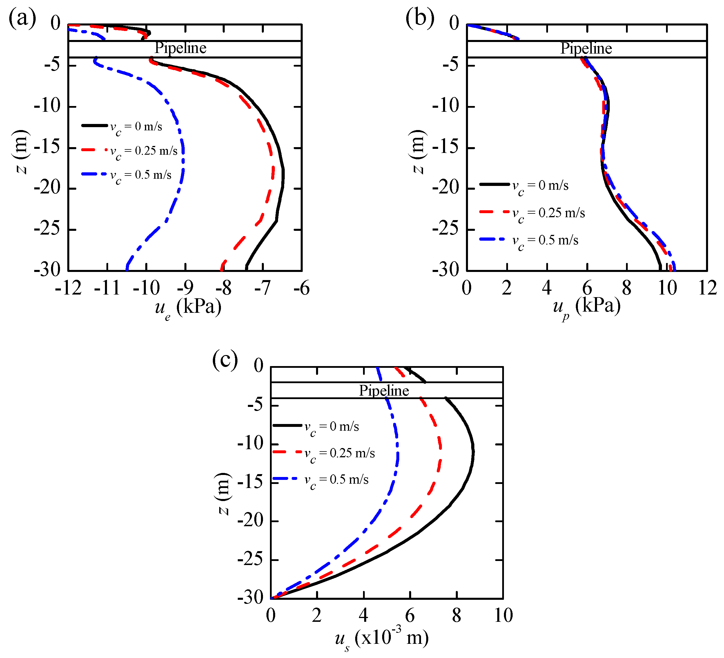
Influence of Current Velocities

Figure 4 shows the influence of different current flow on wave at a specific location over time. The information is extracted from the midpoint of the seabed surface within the computational domain (i.e., x = 150 m). Seabed surface midpoint (x = 150 m) is chosen as the specific point to be analyzed because wave trains are assumed to be more stable as there might be a minor disturbance at the start and end point of the computational domain (i.e., x = 0 m and x = 300 m respectively). At the starting point of the domain (i.e., x = 0 m), wave and current flow are first introduced. A wave absorber is placed after the computational domain (i.e., x = 300 m), which is for the dissipation of wave energy. From Figure 4, it is observed that as the current flow increases, wave pressure also increases.

3.2. Seabed Characteristics

In COMSOL Multiphysics, several simulations were conducted to simulate the wave–current induced soil response, i.e., oscillatory pore pressure and residual pore pressure, and the parameters used are as listed in Table 1, and the current velocity is taken as 0.5m/s in all the following simulations in Section 3.2. The generation of pore pressure in the seabed are sensitive to the seabed characteristics, for instance, soil permeability ($k_s$), shear modulus of the seabed (G), relative density ($D_r$) and degree of saturation ($S_r$). The degree of sensitivity of these parameters on the pore pressure generation is discussed in the following section.

3.2.1. Effects of Soil Permeability

Soil permeability or also known as the hydraulic conductivity is a soil property, which allows the seepage of fluids to pass through its interconnected void spaces. Depending on the soil types, soil permeability can vary on a range from 1.0 × 10⁻¹² to 1.0 × 10⁻² m/s. In this analysis, three different values of soil permeability (i.e., k = 1.0 × 10⁻², 1.0 × 10⁻³ and 1.0 × 10⁻⁴ m/s) are evaluated. Figure 5a,b illustrate the distribution of wave and current induced oscillatory pore pressure and residual pore pressure at the point x = 50 m and z = −10 m respectively under different soil permeability conditions. The results expressed in Figure 5 are for the case in which shear modulus (G) and relative density ($D_r$) set as 5.0 × 10⁶ N/m² and 0.5, respectively.

From Figure 5a, it can be observed that changes in the soil permeability have minimal influence on the value for oscillatory pore pressure. However, as noted in Figure 5b, seabed with low permeability (i.e., k_s = 1.0 × 10⁻⁴ m/s) tends to generate a higher value of residual pore pressure. It is because water cannot dissipate efficiently from low permeable soils and eventually resulted in the build-up of excess pore pressure.

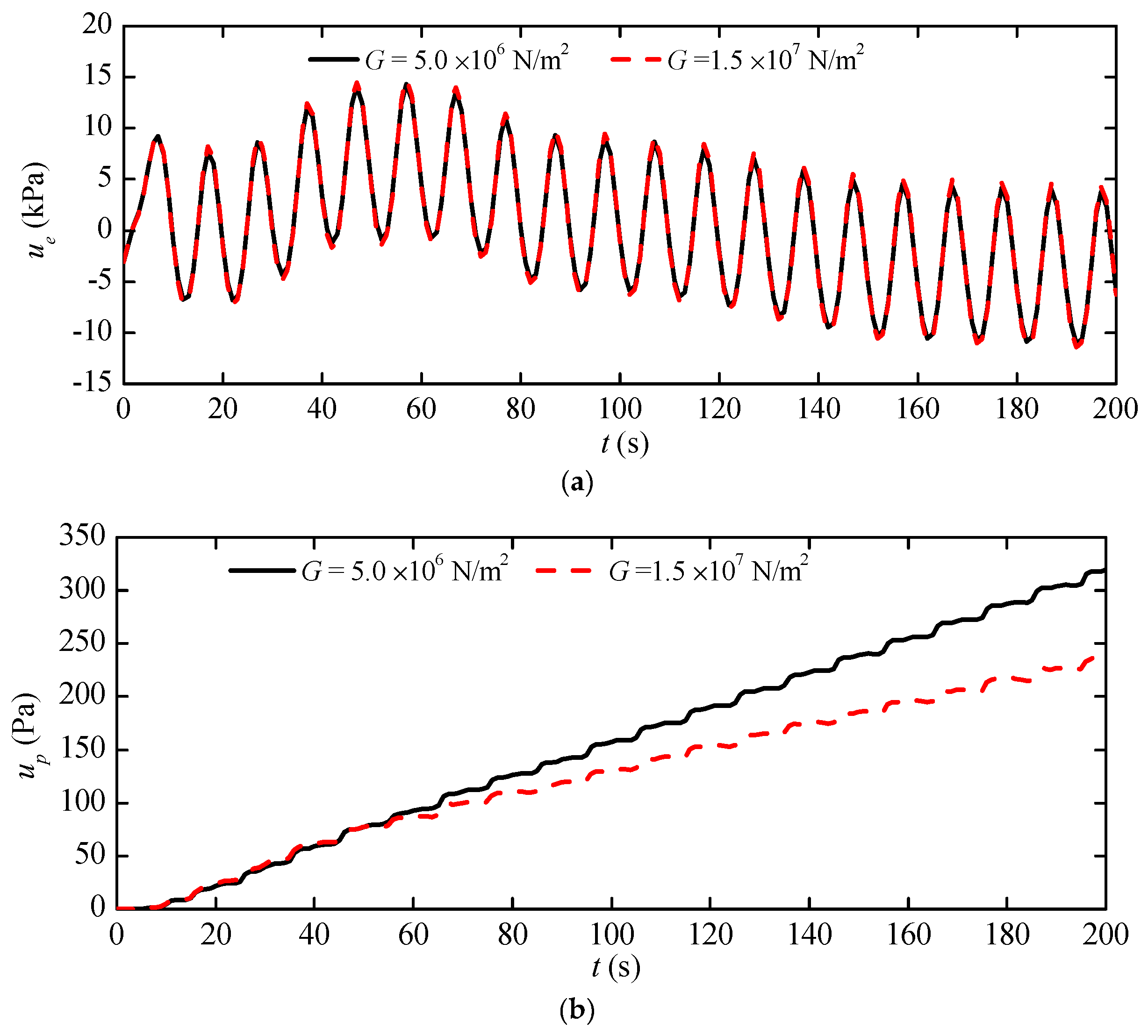
3.2.2. Effects of Shear Modulus

Figure 6 illustrates the variations of wave–current induced pore pressure at x = 50 m and z = −10 m under two different values of shear modulus (i.e., G = 5.0 × 10⁶ and 1.5 × 10⁷ N/m²). In this section, the soil permeability and relative density are fixed at 0.0001 m/s and 0.5 respectively. Shear modulus is one of the soil properties that used to describe the tendency of an object deforms in shape at constant volume when acted upon by the opposing forces. Consider that the soil to be elastic, shear modulus (G) has a relationship with Young’s modulus (E) and Poisson’s ratio (v), which can be calculated from:

$$G=\frac{E}{2\left(1+v\right)}$$

(24)

Therefore, with a fixed value of Poisson’s ratio (v) at 0.35, Young’s modulus can be obtained from Equation (24) as 13.5 MPa and 40.5 MPa for shear modulus (G) of 5.0 × 10⁶ N/m² and 1.0 × 10⁷ N/m² respectively. The soil becomes denser when shear modulus and Young’s modulus increases. From the reference table below (

Table 2. Selected elastic constants for soils (adapted from Das, 2007 [36]).

Type of Soil	Young’s Modulus, E (MPa)	Poisson’s Ratio, v
Loose sand	10.5–24.0	0.20–0.40
Medium dense sand	17.25–27.60	0.25–0.40
Dense sand	34.50–55.20	0.30–0.45
Silty sand	10.35–17.25	0.20–0.40
Sand and gravel	69.00–172.50	0.15–0.35
Soft clay	4.1–20.7	-
Medium clay	20.7–41.4	0.20–0.50
Stiff clay	41.4–96.6	-

), soil with Young’s modulus of 13.5 MPa is said to be loose sand while soil with Young’s modulus of 40.5 MPa is said to be medium dense sand. When loose, saturated soil is subjected to shear force, the soil particles tend to rearrange themselves into a denser manner, i.e., fewer void spaces as the water particles are being forced out of the voids. However, once the pore water drainage is blocked, the pore water pressure will increase progressively with shear force. The stress is transferred from the soil skeleton to pore pressure, which eventually leads to a reduction in effective stress and shear resistance. As for dense sand under monotonically shearing, the soil skeleton contracts and then dilates. The soil volume increases when the soil is saturated with poor drainage, which will result in a decrease in pore pressure. Hence, there is an increase in effective stress and shear strength. Therefore, it concludes that loose sand (contractive) tends to generate higher residual pore pressure than dense sand (dilative).

3.2.3. Effects of Relative Density

Relative density ($D_r$) is a soil parameter that commonly used to indicate the in-situ denseness or looseness of granular soil [37]. It is defined as the ratio of the difference between the void ratios of a cohesionless soil in its loosest state and existing natural state to the difference between its void ratio in the loosest and densest states, which can be formulated as follows:

$$D_r=\frac{e_{max}-e}{e_{max}-e_{min}}$$

(25)

As seen in Equation (17), when there is a change in the relative density of the soil, both the empirical coefficient ${\alpha }_r$ and ${\beta }_r$ in the source term $f\left(x,z,t\right)$ varies, which eventually leads to different values of residual pore pressure. Figure 6 shows the generation of oscillatory and residual pore pressure due to the influence of various relative density ($D_r$ = 0.2, 0.3 and 0.5) over a certain period at point x = 50 m and z = –10 m. In this section, the soil permeability (k) and shear modulus (G) are set as 1.0 × 10⁻⁴ m/s and 5.0 × 10⁶ N/m² respectively while other parameters remain unchanged as shown in Table 1. Figure 7a shows that oscillatory pore pressure is not affected by the change in relative density. However, the generation of residual pore pressure varies drastically as shown in Figure 7b. Higher accumulation of pore pressure is generated when the relative density is of a smaller value, i.e., looser soil. This concludes that loose sand tends to generate higher residual pore pressure (same explanation as Section 3.2.1).

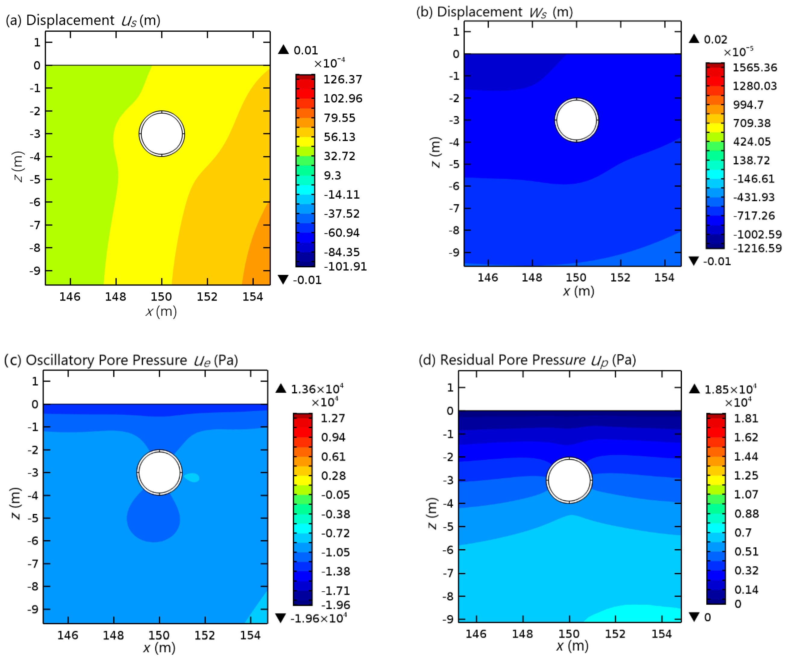
3.3. Around the Vicinity of the Pipeline

In this section, we will study the dynamic soil response around the vicinity of the buried pipeline when the seabed is subjected to wave and current loading. The parameters utilized in the comparison of soil responses such as displacement and pore pressure around the buried pipeline under different current velocity are stated in Table 1, however, the shear modulus, permeability and relative density of the seabed in the simulation are set at a fixed value of 5.0 × 10⁶ N/m², 1.0 × 10^–4 m/s and 0.2 respectively.

As shown in the sketch of wave–current–seabed–pipeline interaction (Figure 2), the pipeline is located at x = 150 m and is embedded 3 m into the ground (Embedment depth is measured from seabed surface to the center of the pipeline). Hence, the analysis is taken at the point x = 150 m at t = 200 s. The graphs in Figure 8 show a comparison between various current velocity ranges from 0 m/s to 0.5 m/s in a gradient of 0.25, which are illustrated in terms of different soil response such as oscillatory pore pressure, residual pore pressure and displacement. The negative values of oscillatory pore pressure in Figure 8a is due to the wave trough phase at that specific time. It can be observed that with lower current values, the oscillatory pore pressure is higher. Figure 8b illustrates the residual pore pressure near the buried pipeline. It can be seen that at the surface of the seabed, residual pore pressure equals to zero. As it goes into the seabed closer to the top of the pipeline, the values increase gradually. The residual pore pressure tends to be higher at the bottom of the pipeline than the top of the pipeline. Figure 8c presents the displacement of seabed when wave and current loading apply on the seabed. It is observed that displacement is higher at the mid-depth of the seabed and gradually decreases to zero as it gets deeper into the seabed. It indicates that at a greater depth, the wave and current loading does not affect the movement of the soil particles.

Figure 9 displays the distribution of wave and current induced seabed responses; oscillatory pore pressure, residual pore pressure, and soil displacements, $u_s$ and $w_s$ around the periphery of the buried pipeline at a duration of 200 s (t = 200 s). Figure 9a,b show the horizontal and vertical soil displacement around the embedded pipeline respectively. There is no significant difference in the soil displacement at the top and bottom of the pipeline. At t = 200 s, a wave trough reaches the proximity of the buried pipeline; therefore, a negative value of oscillatory pore pressure is observed as shown in Figure 9c. As shown in Figure 9d, the residual pore pressure increases gradually with depth because pore water pressure can dissipate efficiently at the seabed surface. Meanwhile, as it goes deeper into the seabed and pipeline, excess pore pressure accumulates which results in an increase in residual pore pressure at the seabed bottom.

4. Conclusions

This research proposes a two-dimensional model with a turbulence closure scheme ($k$-$\epsilon \mathrm{turbulence})$ to investigate the dynamic seabed responses around the vicinity of a buried pipeline under combined wave and current loading. However, according to Alberello et al. [38], there has no visible effect on the two-dimensional model with or without turbulence closure scheme whereas a substantial difference can be seen in a three-dimensional with turbulence model. Therefore, the current two-dimensional model is expected to expand into a three-dimensional model with a turbulence closure scheme in the future.

The effects of current, wave and soil characteristics on the wave–current-induced soil responses are examined. According to the numerical results presented above, the following conclusions can be drawn:

(1)

In the analysis of wave-seabed-structure interaction, the current should be taken into consideration—an increase in the current flow results in an increase in wave pressure. When wave pressure increases, the oscillatory pore pressure tends to increase with increasing current velocity.

(2)

Soil permeability governs the seepage of fluid passing through or flowing out of the seabed. Low permeability, i.e., pore fluids cannot dissipate efficiently, resulted in higher residual pore pressure due to the increase in the buildup of excess pore pressure.

(3)

Shear modulus has a relationship with Young’s modulus and Poisson’s ratio, which describe the rigidity of the seabed. Keeping the Poisson’s ratio as a constant value, a higher value of shear modulus generates a higher value of Young’s modulus, which represents a denser soil. As presented above, loose sand tends to produce a higher value of residual pore pressure.

(4)

Relative density controls the empirical coefficients α_r and β_r in source term, which affects the generation of residual pore pressure. It concludes that a smaller value of relative density results in a higher value of residual pore pressure. However, there is no visible difference in the oscillatory pore pressure.

References

1. Liao, C.; Tong, D.; Chen, L. Pore Pressure Distribution and Momentary Liquefaction in Vicinity of Impermeable Slope-Type Breakwater Head. Appl. Ocean Res. 2018, 78, 290–306. [Google Scholar] [CrossRef]
2. Liao, C.; Chen, J.; Zhang, Y. Accumulation of pore water pressure in a homogenous sandy seabed around a rocking mono-pile subjected to wave loads. Ocean Eng. 2019, 173, 810–822. [Google Scholar] [CrossRef]
3. Guo, Z.; Jeng, D.S.; Zhao, H.Y.; Guo, W.; Wang, L.Z. Effect of Seepage Flow on Sediment Incipient Motion around a Free Spanning Pipeline. Coast. Eng. 2019, 143, 50–62. [Google Scholar] [CrossRef]
4. Chen, W.Y.; Chen, G.X.; Chen, W. Numerical simulation of the non-linear wave-induced dynamic response of anisotropic poro-elastoplastic seabed. Mar. Georesour. Geotechnol. 2018, 1–12. [Google Scholar] [CrossRef]
5. Wong, Z.S.; Liao, C.C.; Jeng, D.S.-D. Poro-Elastoplastic Model for Short-Crested Wave-Induced Pore Pressures in a Porous Seabed. Open Civ. Eng. J. 2015, 9, 408–416. [Google Scholar] [CrossRef]
6. Zen, K.; Yamazaki, H. Mechanism of wave-induced liquefaction and densification in seabed. Soils Found. 1990, 30, 90–104. [Google Scholar] [CrossRef]
7. Jeng, D.-S. Porous Models for Wave-Seabed Interactions; Springer: Berlin/Heidelberg, Germany, 2013; Volume 9783642335, ISBN 978-3-642-33592-1. [Google Scholar]
8. Yang, G.; Ye, J. Wave & current-induced progressive liquefaction in loosely deposited seabed. Ocean Eng. 2017, 142, 303–314. [Google Scholar] [CrossRef]
9. Zhang, X.; Zhang, G.; Xu, C. Stability analysis on a porous seabed under wave and current loadings. Mar. Georesour. Geotechnol. 2017, 35, 710–718. [Google Scholar] [CrossRef]
10. Wen, F.; Wang, J.H. Response of Layered Seabed under Wave and Current Loading. J. Coast. Res. 2015, 314, 907–919. [Google Scholar] [CrossRef]
11. Ye, J.H.; Jeng, D.-S. Response of Porous Seabed to Nature Loadings: Waves and Currents. J. Eng. Mech. 2012, 138, 601–613. [Google Scholar] [CrossRef]
12. Tong, D.; Liao, C.; Chen, J.; Zhang, Q. Numerical Simulation of a Sandy Seabed Response to Water Surface Waves Propogating on Current. J. Mar. Sci. Eng. 2018, 6, 88. [Google Scholar] [CrossRef]
13. Zhang, Y.; Jeng, D.S.; Gao, F.P.; Zhang, J.S. An analytical solution for response of a porous seabed to combined wave and current loading. Ocean Eng. 2013, 57, 240–247. [Google Scholar] [CrossRef] [Green Version]
14. Liao, C.C.; Jeng, D.-S.; Zhang, L.L. An Analytical Approximation for Dynamic Soil Response of a Porous Seabed due to Combined Wave and Current Loading. J. Coast. Res. 2015, 315, 1120–1128. [Google Scholar] [CrossRef]
15. Zhou, X.L.; Wang, J.H.; Zhang, J.; Jeng, D.S. Wave and current induced seabed response around a submarine pipeline in an anisotropic seabed. Ocean Eng. 2014, 75, 112–127. [Google Scholar] [CrossRef]
16. Liu, B.; Jeng, D.-S.; Ye, G.L.; Yang, B. Laboratory study for pore pressures in sandy deposit under wave loading. Ocean Eng. 2015, 106, 207–219. [Google Scholar] [CrossRef]
17. Gao, F.P.; Yan, S.; Yang, B.; Wu, Y. Ocean Currents-Induced Pipeline Lateral Stability on Sandy Seabed. J. Eng. Mech. 2007, 133, 1086–1092. [Google Scholar] [CrossRef]
18. Zhou, C.; Li, G.; Dong, P.; Shi, J.; Xu, J. An experimental study of seabed responses around a marine pipeline under wave and current conditions. Ocean Eng. 2011, 38, 226–234. [Google Scholar] [CrossRef]
19. Youssef, B.S.; Tian, Y.; Cassidy, M.J. Centrifuge modelling of an on-bottom pipeline under equivalent wave and current loading. Appl. Ocean Res. 2013, 40, 14–25. [Google Scholar] [CrossRef]
20. Sassa, S.; Sekiguchi, H. Wave-induced liquefaction of beds of sand in a centrifuge. Géotechnique 1999, 49, 621–638. [Google Scholar] [CrossRef]
21. Yang, B.; Luo, Y.; Jeng, D.; Feng, J.; Huhe, A. Experimental studies on initiation of current-induced movement of mud. Appl. Ocean Res. 2018, 80, 220–227. [Google Scholar] [CrossRef]
22. Zhao, H.-Y.; Jeng, D.-S.; Guo, Z.; Zhang, J.-S. Two-Dimensional Model for Pore Pressure Accumulations in the Vicinity of a Buried Pipeline. J. Offshore Mech. Arct. Eng. 2014, 136, 042001. [Google Scholar] [CrossRef]
23. Zhao, H.-Y.; Jeng, D.-S. Accumulated pore pressures around submarine pipeline buried in trench layer with partial backfills. J. Eng. Mech. 2016, 142, 04016042. [Google Scholar] [CrossRef]
24. Zhou, X.-L.; Zhang, J.; Guo, J.-J.; Wang, J.-H.; Jeng, D.-S. Cnoidal wave induced seabed response around a buried pipeline. Ocean Eng. 2015, 101, 118–130. [Google Scholar] [CrossRef]
25. Duan, L.; Liao, C.; Jeng, D.-S.; Chen, L. 2D numerical study of wave and current-induced oscillatory non-cohesive soil liquefaction around a partially buried pipeline in a trench. Ocean Eng. 2017, 135, 39–51. [Google Scholar] [CrossRef]
26. Duan, L.; Jeng, D.-S.; Liao, C.; Zhu, B.; Tong, D. Three-dimensional poro-elastic integrated model for wave and current-induced oscillatory soil liquefaction around offshore pipeline. Appl. Ocean Res. 2017, 68, 293–306. [Google Scholar] [CrossRef]
27. Benra, F.-K.; Dohmen, H.J.; Pei, J.; Schuster, S.; Wan, B. A Comparison of One-way and Two-Way Coupling Methods for Numerical Analysis of Fluid-Structure Interactions. J. Appl. Math. 2011, 1–16. [Google Scholar] [CrossRef]
28. Jones, W.P.; Launder, B.E. The predictions of Laminarization with a two-equation model of turbulence. Int. J. Heat Mass Transf. 1972, 15, 301–314. [Google Scholar] [CrossRef]
29. Lin, P.; Liu, P.L.F. A numerical study of breaking wave in the surf zone. J. Fluid Mech. 1998, 359, 239–264. [Google Scholar] [CrossRef]
30. Biot, M.A. General Theory of Three-Dimensional Consolidation. J. Appl. Phys. 1941, 12, 155–164. [Google Scholar] [CrossRef]
31. Jeng, D.-S. Mechanics of Wave-Seabed-Structure Interactions: Modelling, Processes and Applications; Cambridge University Press: Cambridge, UK, 2018; ISBN 978-1-107-16000-2. [Google Scholar]
32. Sumer, B.M.; Kirca, V.S.O.; Fredsøe, J. Experimental Validation of a Mathematical Model Liquefaction Under Waves. Int. J. Offshore Polar Eng. 2012, 22, 133–141. [Google Scholar]
33. Hirt, C.W.; Nichols, B.D. Volume of fluid (VOF) method for the dynamics of free boundaries. J. Comput. Phys. 1981, 39, 201–225. [Google Scholar] [CrossRef]
34. Paulsen, B.T.; Bredmose, H.; Bingham, H.; Jacobsen, N. Forcing of a bottom-mounted circular cylinder by steep regular water waves at finite depth. J. Fluid Mech. 2014, 755, 1–34. [Google Scholar] [CrossRef]
35. COMSOL Inc. COMSOL Multiphysics 5.3 User Guide Manual; COMSOL Inc.: Burlington, MA, USA, 2014. [Google Scholar]
36. Das, B.M. Principles of Foundation Engineering; Thomson/Brooks/Cole: Pacific Grove, CA, USA, 2007; ISBN 978-0-495-08246-0. [Google Scholar]
37. Das, B.M. Principles of Geotechnical Engineering-SI Version, 7th ed.; Cengage Learning: Boston, MA, USA, 2014; ISBN 978-1-133-10867-2. [Google Scholar]
38. Alberello, A.; Pakodzi, C.; Nelli, F.; Bitner-Gregersen, E.M.; Toffoli, A. Threee Dimensional Velocity Field Underneath a Breaking Rogue Wave. In Proceedings of the ASME 2017 36th International Conference Ocean, Offshore and Arctic Engineering, Trondheim, Norway, 25–30 June 2017; Volume 3A: Structures, Safety and Reliability. p. V03AT02A009. [Google Scholar] [CrossRef]
Figure 1. The conceptual sketch of the pore pressure mechanisms (Adapted from Jeng [7]).
Jmse 07 00066 g001
Figure 2. Sketch of the wave–current–seabed–pipeline interactions.
Jmse 07 00066 g002
Figure 3. Comparison between different mesh sizes for COMSOL Multiphysics in terms of (a) the number of elements and the computational time, and (b) residual pore pressure, u p at a duration of 100 s.
Jmse 07 00066 g003
Figure 4. Variation of wave pressure,   p at the seabed bottom for different current velocities.
Jmse 07 00066 g004
Figure 5. Variations of (a) oscillatory pore pressure, u e and (b) residual pore pressure, u p at a specific point for different soil permeability.
Jmse 07 00066 g005
Figure 6. Variations of (a) oscillatory pore pressure,   u e and (b) residual pore pressure, u p at a specific point under the different shear modulus.
Jmse 07 00066 g006
Figure 7. Variation of (a) oscillatory pore pressure, u e and (b) residual pore pressure, u p _p at a specific point under the different relative density.
Jmse 07 00066 g007
Figure 8. Variation in (a) oscillatory pore pressure, u e , (b) residual pore pressure, u p and (c) displacement, u s under various current velocity.
Jmse 07 00066 g008
Figure 9. Distribution of seabed responses such as (a) horizontal displacement u s , (b) vertical displacement w s , (c) oscillatory pore pressure,   u e , and residual pore pressure u p around the vicinity of the buried pipeline due to wave and current loading when current velocity is set at v c = 0.5 m/s.
Jmse 07 00066 g009