Article

Meshfree Model for Wave-Seabed Interactions Around Offshore Pipelines

1
School of Engineering and Built Environment, Griffith University Gold Coast Campus, Queensland 4222, Australia
2
Department of Marine Environmental Engineering, National Kaohsiung University of Science and Technology, Kaohsiung 824, Taiwan
3
Department of Marine Environment and Engineering, National Sun Yat-Sen University, Kaohsiung 804, Taiwan
*
Author to whom correspondence should be addressed.
J. Mar. Sci. Eng. 2019, 7(4), 87; https://doi.org/10.3390/jmse7040087
Submission received: 26 February 2019 / Revised: 21 March 2019 / Accepted: 22 March 2019 / Published: 28 March 2019
(This article belongs to the Special Issue Coastal Geohazard and Offshore Geotechnics)

Abstract

:
The evaluation of the wave-induced seabed instability around a submarine pipeline is particularly important for coastal engineers involved in the design of pipelines protection. Unlike previous studies, a meshfree model is developed to investigate the wave-induced soil response in the vicinity of a submarine pipeline. In the present model, Reynolds-Averaged Navier-Stokes (RANS) equations are employed to simulate the wave loading, while Biot’s consolidation equations are adopted to investigate the wave-induced soil response. Momentary liquefaction around an offshore pipeline in a trench is examined. Validation of the present seabed model was conducted by comparing with the analytical solution, experimental data, and numerical models available in the literature, which demonstrates the capacity of the present model. Based on the newly proposed model, a parametric study is carried out to investigate the influence of soil properties and wave characteristics for the soil response around the pipeline. The numerical results conclude that the liquefaction depth at the bottom of the pipeline increases with increasing water period (T) and wave height (H), but decreases as backfilled depth ( H b ), degree of saturation ( S r ) and soil permeability (K) increase.

1. Introduction

Offshore pipelines have been a commonly used facility for transportation of offshore oil and gas. In addition to construction causes, another key failure mode is the wave-induced seabed instability in the vicinity of pipelines [1,2]. Therefore, the evaluation of seabed stability around the pipeline is one of key factors that needs to be considered in an offshore pipeline project.
In general, ocean waves will exert fluctuations of dynamic pressures over the sea floor, which will further induce excess pore pressures and effective stresses within the seabed. The shear resistance in the vicinity of pipelines may be loss due to the liquefaction of surrounding soil, when the excess pore pressure increases. Thus, it is particularly important to understand the process of the wave-pipeline-soil interactions for the design of submarine pipelines [3]. The mechanisms of the wave-induced soil liquefaction can be classified into two categories, residual and oscillatory, in accordance with the way how the excess pore pressure is generated [4]. The residual liquefaction mechanism is resulted from the build-up of pore pressure induced by volumetric contraction under cyclic loading [5]. Momentary liquefaction usually appears in the seabed under wave troughs where the pore pressure is accompanied with some damping and phase lag [6]. This study focuses on the second mechanism.
Numerous investigations for the wave-induced soil response around submarine pipelines by adopting conventional numerical methods have been carried out since the 1980s, such as finite-element method (FEM), finite difference method (FDM) and boundary element method (BEM). Among these, Cheng and Liu [7] introduced the Boundary Integral Equation to obtain the distribution of pore-water pressure around a pipe fully buried in a sediment-filled trench. In their model, the inertia terms were considered, i.e., it is a u p approximation. Thomas [8,9] established a one-dimensional finite-element model to analyze the wave-induced soil response in saturated and unsaturated soil. Later, the model was extended to investigate the influences of variable permeability and shear modulus of soil and non-linearity of wave loading [10,11]. Furthermore, by using finite-element formulation, Madga [12,13,14] further estimated the wave-induced pore pressure and uplift force acting on submarine pipelines. Based on the assumption of no slipping at the interface between pipeline and soil, Jeng and Lin [15] developed a finite-element model to examine the wave-pipeline-seabed interactions in an in-homogeneous seabed. Then, the inertial forces and soil-pipe contact effects were involved in Luan et al. [16]’s model. With the commercial software (ABQUS), the effects of combined non-linear wave and current loading were considered by Wen et al. [17]. Recently, by considering pre-consolidation due to self-weight of the pipeline, Zhao et al. [18] investigated the build-up pore pressures. Recently, Zhao and Jeng [19] extended the integrated numerical model to evaluate the influence of backfilled depth of trench layer. Later, Duan et al. [20] proposed a two-dimensional model to investigate the wave and current-induced soil response around a partially buried pipeline in a trench layer.
The aforementioned investigations have employed the conventional approaches with meshes, for example, the principle of FEM is to divide the computational domain into small elements, and these elements do not overlap each other. A field function was established within each element by adopting simple interpolation functions. If the element is severely distorted, the shape function of this element would be of poor quality, which may lead to an unacceptable numerical result. Unlike the finite-element technique, the interpolation functions are established directly on nodes instead of elements, when meshless methods are applied. This could avoid the drawback of the conventional mesh-based techniques such as FEM and FDM. In recent years, meshless methods have attracted increasing attention from numerical modelers due to the faster formulation process with less data storage and no extensive mesh.
The most commonly used meshless methods are method of fundamental solution (MFS), method of particular solutions (MPS), smooth particle hydrodynamics (SPH), global radial basis functions (RBF) collocation method (GRBFCM) and local RBF collocation method (LRBFCM). One of the earliest meshless methods is SPH [21,22]. Randles and Libersky [23] was the first group to apply SPH in solid mechanics, and later this method was improved and was adopted in more fields. The main drawbacks of this method are inaccurate results near boundaries and tension instability, which was first studied in 1995. Over the ensuring decades, more meshless methods have been proposed. Karim et al. [24] presented a two-dimensional model using the element-free Galerkin method to investigate transient response of saturated porous elastic soil under cyclic loading system. A radial point interpolation meshless method (radial PIM) was developed by Wang et al. [25] to avoid the occurrence of singularity associated with only polynomial basis. Later, the radial PIM was applied to solve Biot’s consolidation problem [26] and wave-induced seabed response [27]. Existing meshless models have investigated water-soil interaction without any structure. Thus, the present study firstly establishes a meshless model to investigate the wave-seabed-pipeline interactions under various wave loading.
Among meshfree methods, the RBF are commonly used. The global RBF collocation method was first proposed for multivariate data interpolation and partial differential equations [28,29]. This method was further modified [30,31,32]. The GRBFCM can be used to deal with arbitrary and complex domains, but it usually leads to an ill-conditioned system matrix when high resolutions are required. Later, a localization procedure (LRBFCM) was proposed to overcome prescribed difficulty, to transform the dense system matrices into sparse ones [33]. Based on the multi-quadric RBF [34], Lee et al. [33] first proposed the local RBF collocation method (LRBFCM), and then this method was applied to various problems [35,36,37].
In this study, LRBFCM is employed to investigate the wave-induced oscillatory liquefaction around a pipeline in a trench layer. The proposed seabed model is validated with the analytical solution [38], experimental data [39,40] and numerical models [7,41]. Then, a parametric study is conducted to evaluate the influence of pipeline configuration, wave characteristics, and seabed properties for the wave-induced pore pressure around a partially buried pipeline in a trench.

2. Theoretical Models

In this study, an impermeable pipeline is considered with a radius of R which is partially buried in a trench with a finite thickness (h), as shown in Figure 1. The propagation direction of waves is along the positive x-direction.
The present model consists of two sub-models: wave and seabed sub-models. By using open-source CFD toolbox OpenFoam (Open Field Operation and Manipulation), the wave model proposed by Higuera et al. [42] is adopted for generating various wave loadings. A new seabed model is established based on LRBFCM.
By means of Volume-Averaged Reynolds-Averaged Navier-Stokes (VARANS) equations, the wave model was developed for coastal engineering applications by dealing with three-dimensional two-phase flow which was based on a solver in OpenFOAM, IHFOAM [42]. More detailed information about IHFOAM and its applications in coastal engineering, readers can refer to the publications of Higuera and his co-workers [42,43,44,45].

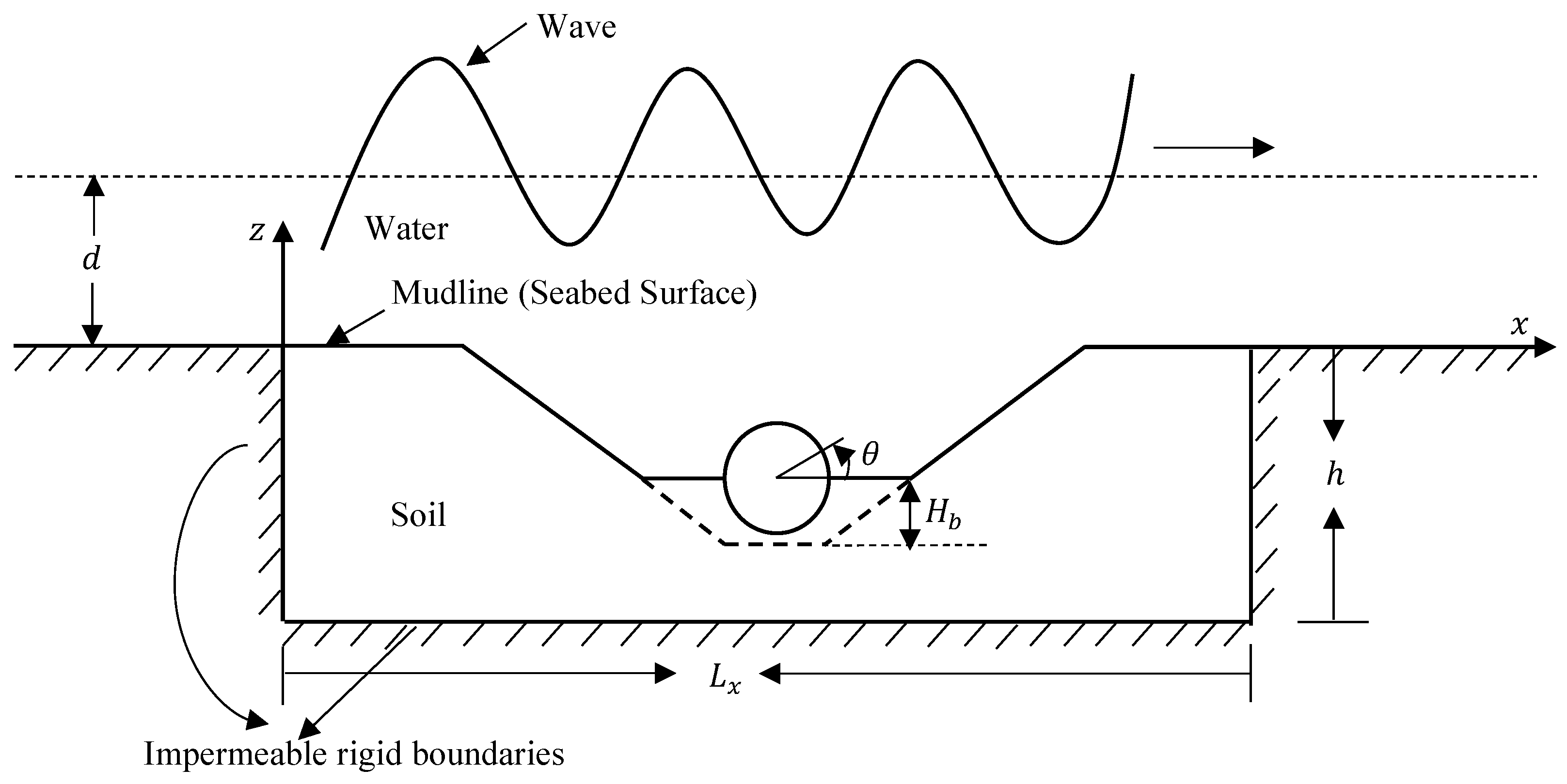
2.1. Boundary Value Problem for the Seabed Model

By neglecting the inertial effect, a quasi-static seabed model is established for the wave-induced seabed response based on the assumption of homogeneous seabed and compressible pore fluid. The effects of inertial terms on the wave-induced soil response has been reported in Jeng et al. [46]. For a two-dimensional problem, the governing equation for compressible homogeneous soil and compressible pore fluid can be represented as [47]:
K 2 p γ w n β p t γ w ϵ t = 0 ,
where p is pore-water pressure, γ w is the unit weight of water, n is soil porosity, t is the time. In (1), the volume strain ( ϵ ) and compressibility of pore fluid ( β ) are defined as
ϵ = u x + w z , and β = 1 K w + 1 S r P w o ,
where u and w are the soil displacements in the x- and z-direction, respectively; K w is the true modulus of elasticity ( K w = 2 × 10 9 N / m 2 , [6]), S r is the degree of saturation and P w o is related to the absolute water pressure.
Based on Newton’s second law, the force balance for the porous flow in x and z directions can be expressed respectively as
σ x x + τ x z z = p x ,
τ x z x + σ z z = p z ,
where σ x and σ z are effective normal stresses; τ x z denotes shear stress component. In this study, tension is determined as positive.
Based on Hook’s law, the effective normal stresses and shear stress can be expressed in term of soil displacements, i.e.,
σ x = 2 G u x + μ 1 2 μ ϵ ,
σ z = 2 G w z + μ 1 2 μ ϵ ,
τ x z = G u z + w x ,
where the shear modulus G is defined with Young’s modulus (E) and the Poisson’s ratio ( μ ) in the form of E / 2 ( 1 + μ ) .
Substituting (5)~(7) into (3) and (4), the force equilibrium can be represented as
G 2 u + G 1 2 μ ϵ x p x = 0 ,
G 2 w + G 1 2 μ ϵ z p z = 0 .
To solve the pore pressures and soil displacements in (1), (8) and (9), the following boundary conditions are required.
  • At seabed surface ( z = 0 ) and trench surface, the vertical effective stress and shear stress vanish, and the pore pressure is equal to dynamic wave pressure.
    σ z = τ x z = 0 , and p = P b ,
    where P b is the dynamic wave pressure at the seabed surface, which is obtained from the wave model (IHFOAM).
  • At the impermeable seabed bottom ( z = h ), zero displacements and no vertical flow are specified, i.e.,
    u = w = 0 , and p z = 0 ,
  • The pipeline surface is assumed to be impermeable wall. Thus, there is no flow through the pipeline surface, i.e.,
    p n = 0 ,
    where n denotes normal vector of the pipe surface.

2.2. Meshfree Model for the Seabed Domain

In this study, a rigid pipeline is considered to be partially buried in a trench. The computational domain is discretized into N nodes non-uniformly. Therefore, a linear equation of the following form is required to be established:
A N × N Φ N × 1 = B N × 1 ,
where Φ N × 1 is the sought solution, B N × 1 is a column vector, and A N × N is a sparse system matrix. Similar structures of A N × N can be found in the FDM and the finite-element method.
For constructing a linear equation for each node y n in the computational domain, Φ in (13) is assumed as Φ ( x ) by RBFs:
Φ ( x ) m = 1 K ¯ α m χ ( r m ) ,
where Φ denotes either p or u i in the governing equations, α m refers to the corresponding undetermined coefficient and r m = x x m is the Euclidean distance from x to x m . The group of x m denote the locations of the K ¯ nearest neighbor nodes surrounding the prescribed center x 1 . In this study, the kd-tree algorithm is applied to search the K ¯ nearest neighbor nodes efficiently [48]. Furthermore, the multi-quadric RBF is expressed as
χ ( r m ) = r m 2 + c 2 ,
with the shape parameter (c) [34].
A localization process [33,35,49] is presented here for the sake of preventing unnecessary ill-conditioned system matrix. Firstly, the expression of r m is substituted into (14) as
Φ ( x n ) = m = 1 K ¯ α m χ ( x m x n ) ,
or in matrix-vector form as
Φ K ¯ × 1 = χ K ¯ × K ¯ α K ¯ × 1 ,
where
Φ K ¯ × 1 = Φ ( x 1 ) Φ ( x 2 ) Φ ( x K ¯ ) ,
χ K ¯ × K ¯ = χ ( x 1 x 1 ) χ ( x 1 x 2 ) χ ( x 1 x K ¯ ) χ ( x 2 x 1 ) χ ( x 2 x 2 ) χ ( x 2 x K ¯ ) χ ( x K ¯ x 1 ) χ ( x K ¯ x 2 ) χ ( x K ¯ x K ¯ ) ,
and
α K ¯ × 1 = α 1 α 2 α K ¯ .
Then, (17) can be inverted as
α K ¯ × 1 = χ K ¯ × K ¯ 1 Φ K ¯ × 1 .
Now, L Φ ( x ) is considered to replace Φ ( x ) defined in (14), where L is a linear differential operator related to both the governing equation and the boundary conditions. The collocation of L Φ ( x ) on x 1 = y n gives
L Φ ( y n ) = m = 1 K ¯ α m L χ ( r m ) x = x 1 ,
or in matrix-vector form as
L Φ ( y n ) = L χ 1 × K ¯ α K ¯ × 1 .
In (23), the existence of L χ ( r m ) is as a result of the influence of operator L on the RBF χ ( r m ) . Thus, (17) and (23) can be combined as
L Φ ( y n ) = C 1 × K ¯ Φ K ¯ × 1 ,
with
C 1 × K ¯ = L χ 1 × K ¯ χ K ¯ × K ¯ 1 ,
and
L χ 1 × K ¯ = L χ ( r 1 ) x = x 1 L χ ( r 2 ) x = x 2 L χ ( r K ¯ ) x = x K ¯ .
From (24)–(26), it can be found that the row vector C 1 × K ¯ can be obtained if all the values of L, χ and x j are known. These equations can be assembled into the system matrix, and finally the resultant sparse system is solved by using the direct solver of SuperLU in this study, which finished the procedure of LRBFCM.
Please note that the radial PIM was adopted to solve Biot’s consolidation problem [26] and wave-induced soil response [27], while the present model uses LRBFCM. The mixed bases of polynomial and radial bases are needed in the radial PIM for the accuracy of polynomials [25]. Compared with the radial PIM, the choice of basis functions in LRBFCM is easier. Furthermore, no submarine structure was included in their model [27]. Thus, the present seabed model is the first model by applying LRBFCM to investigate the wave-seabed interactions around a structure such as pipelines.

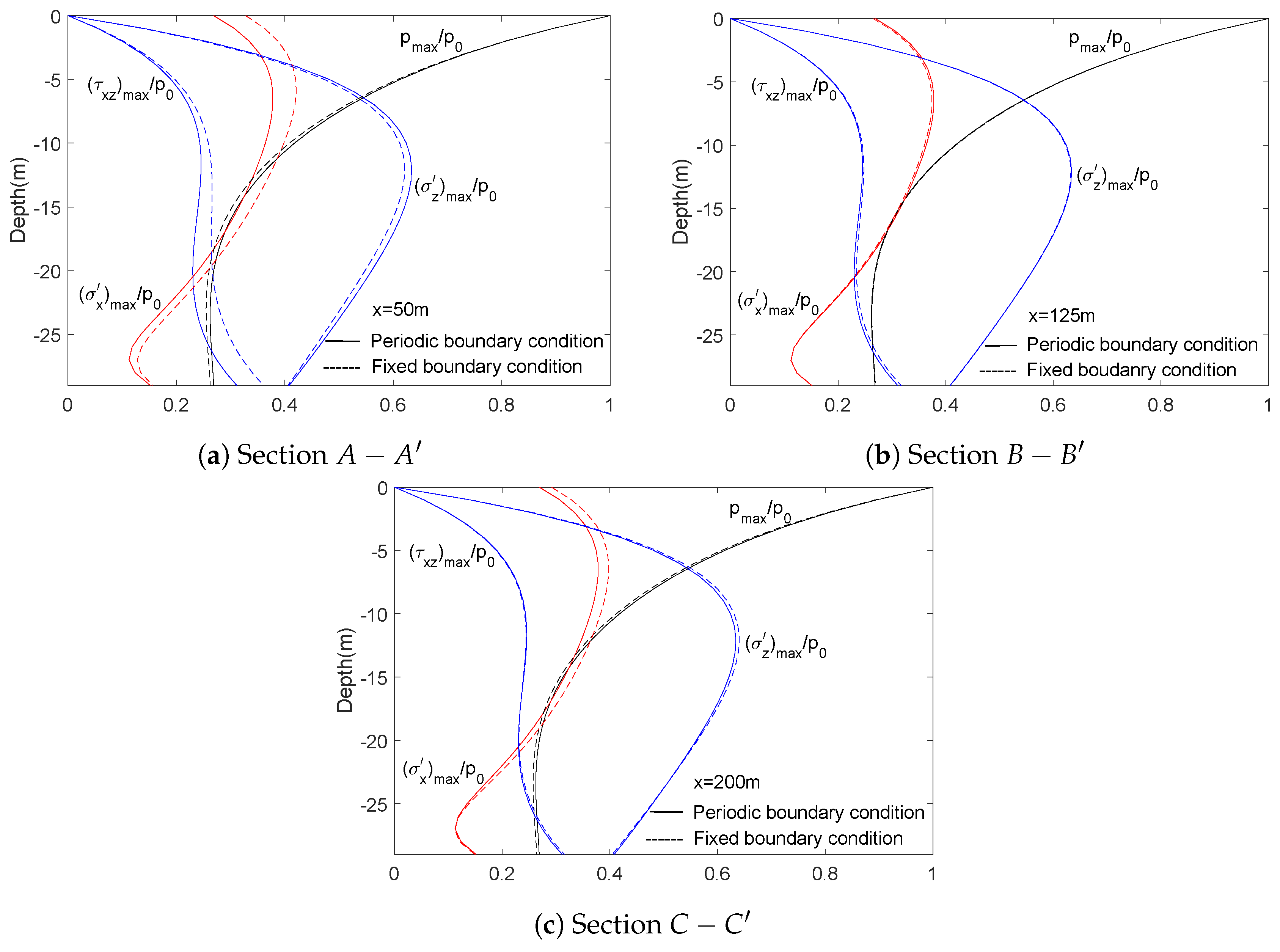
2.3. Effects of Lateral Boundary Conditions

This section presents two ways to handle the lateral boundary conditions: periodic and fixed. Generally speaking, the horizontal and vertical displacements and the pore pressure do not vanish at lateral boundaries. To deal with the problem of boundaries for wave-seabed interactions, Jeng et al. [50] applied the principle of repeatability [51]. However, the condition of employing periodic boundary condition is that the length of seabed must be an integer number of wavelength. Moreover, periodic boundary condition is not applicable for seabed with structures. Thus, Ye and Jeng [52] suggested another method by which employing a large computational domain and meanwhile fixing both the lateral boundaries in the horizontal direction, namely considering the boundary as impermeable. This method is under the assumption that the fixed lateral boundary only influences the region nearby. Similar with Ye and Jeng [52], in this section, both periodic and fixed lateral boundary conditions by LRBFCM are examined.
Theoretically, the larger the computational domain, the smaller effects of lateral boundaries. However, a large computational domain requires more computational resources. Thus, the length of computational domain is assumed as 3 times of the periodic wavelength in this study. The input data used is listed in Table 1. The maximum pore pressure and effective stresses of soil of these three sections are depicted in Figure 2.
As depicted in Figure 2, sections A A ( x = 50 m), B B ( x = 125 m) and C C ( x = 200 m) are in the range of the first wave length, the second wavelength and the third wavelength, separately. Solid lines and dashed lines represent the soil response of the case with periodic and fixed boundaries, respectively. As shown in Figure 2a,c, the effect of fixed boundary condition is minor for vertical effective stress and pore pressure in sections A A and C C , but considerable difference can be observed from the horizontal effective stress, which leads to the conclusion that fixed lateral boundaries affect the soil response of the soil region near lateral boundaries significantly. Furthermore, the seabed response at section B B under periodic boundary conditions is in a complete agreement with that under fixed boundary conditions, which means that the influence of fixed lateral boundaries vanish in the section far away from the boundary. Thus, fixed lateral boundary condition is employed in this study for investigating the wave-induced soil response.

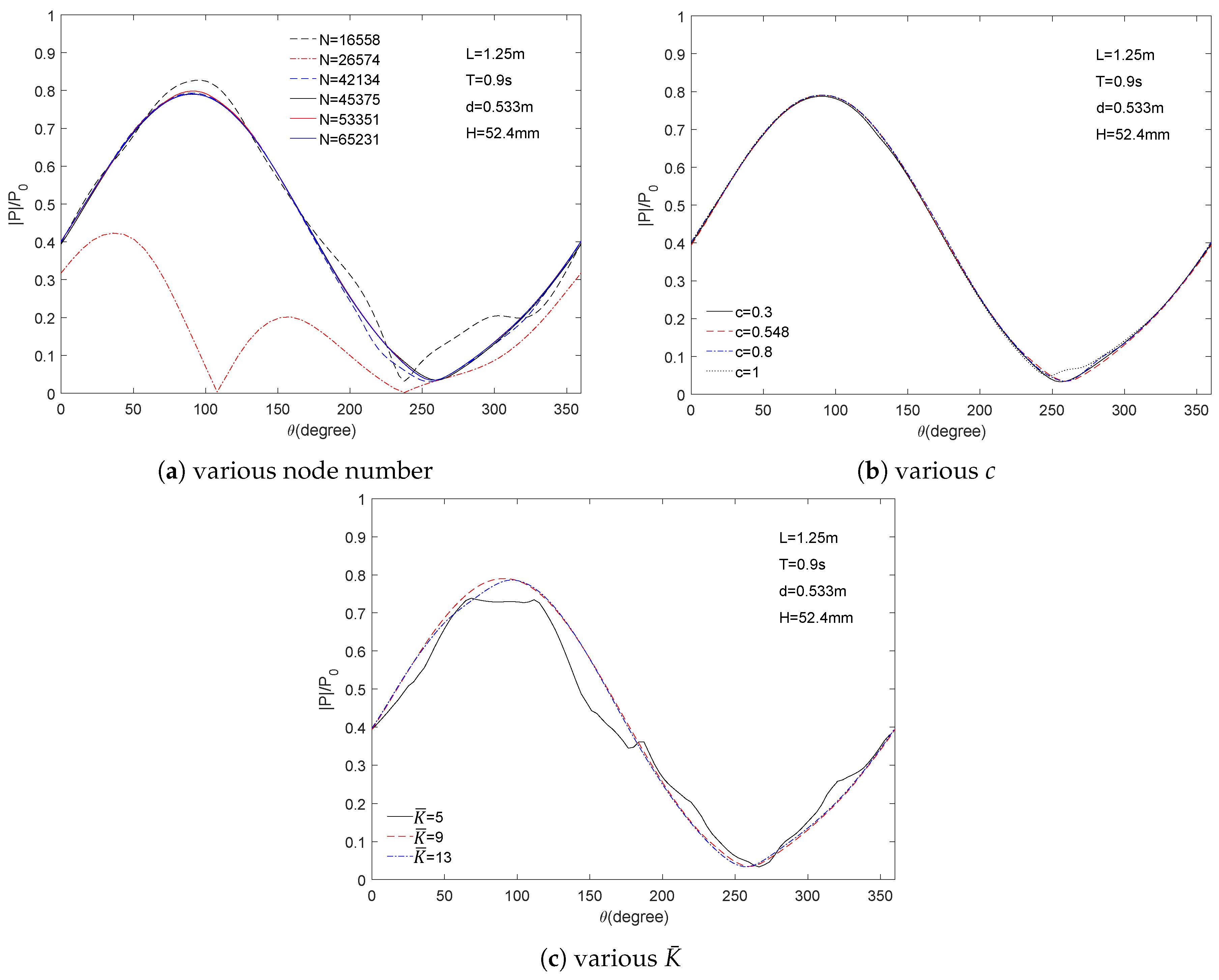
2.4. Convergent Tests

The present seabed model is a new model established by employing LRBFCM for the wave-induced soil response in the vicinity of submarine pipelines, it is necessary to check its convergence. Figure 3 presents three tests for model convergence which is with respect to node number of the whole computational domain, a model parameter c (where c is equal to “ 30 × the maximum distance between each two nodes in the local region”) and the value of K ¯ (where K ¯ indicates the node number of the local region). The pipeline is considered to be impermeable, and input data are as follows: d = 0 . 533 m, L = 1 . 25 m, h = 0 . 826 m, μ = 0 . 33 , n = 0 . 42 , K = 0 . 0011 m/s, S = 0 . 997 , R = 0 . 084 m, b = 0 . 167 m, L x = 4 . 57 m.
In principle, instability of the trend of soil response around pipeline occurs at the beginning stage of node number increase. The results should remain unchanged after the node number is increased to a certain extent. With fixed node numbers, the numerical results should not be changed when the value of c is in a reasonable range, which can prove that the model is convergent and reliable. As presented in Figure 3a, the wave-induced pore pressure keep changed when the node number varies from 16,558 to 45,000 approximately, but the values maintain a steady state in the process of the node number increases from 45,375 to 53,351 and even 65,231, which verifies the stability of the model. c is one of coefficients of the present model. In Figure 3b, the node number is determined as 45,375, then the trend of pore pressure can be observed through changing the value of c. There is almost no change for the pore pressure in the vicinity of the pipeline when c is equal to 0.3, 0.548 and 0.8, respectively, which can be evidence of the model convergence. K ¯ refers to the number of the nearest neighbor nodes of unknown node x. Usually, the value of K ¯ can be regarded as 5, 9, and 13. From Figure 3c, it can be found that 9 or 13 is applicable for the present model, and the result looks more smooth when K ¯ is equal to 9. Thus, the convergence of present model is verified from these three cases. Combined Figure 3a–c, it can be concluded that the numerical result of this case scale is satisfactory when the node number, and the value of c and K ¯ are determined as 45375, 0.548 and 9, respectively.

3. Model Validation

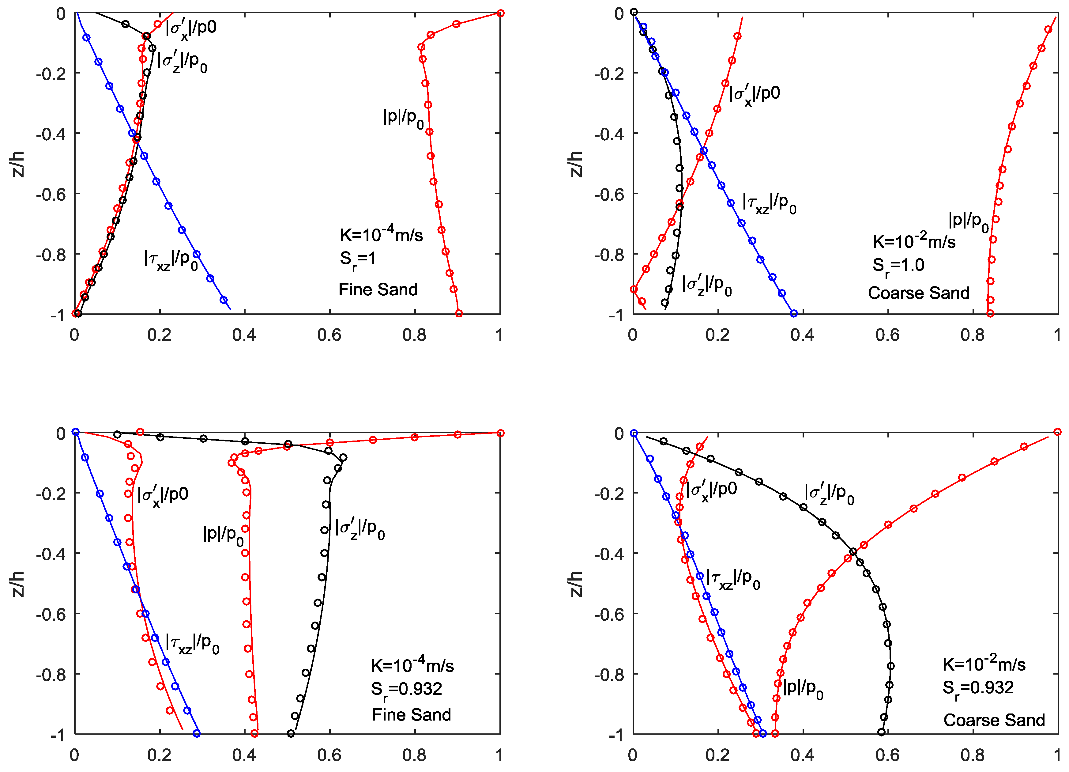
3.1. Comparison with the Analytical Solution for Wave-Seabed Interactions

For a homogeneous seabed, the previous analytical solution for the wave-induced soil response [38] will be compared with present numerical results. This comparison is to confirm the capacity of the present model.
In this comparison, the following input data are used: wave period T = 15 . 0 sec, water depth d = 70 m, wavelength L = 311 . 59 m, thickness of seabed h = 25 m, Poisson’s ratio μ = 0 . 333 , soil porosity n = 0 . 3 , soil permeability K = 10 4 m/s for fine sand and 10 2 m/s for coarse sand, degree of saturation S = 0 . 932 for unsaturated soil, shear modulus G = 10 7 N / m 2 . The numerical results of the comparison are presented in Figure 4. In the figure, the present results are presented by lines and the analytical solution [38] is denoted as circles. The vertical distributions of the maximum amplitude of the wave-induced pore pressure ( | p | / p 0 ) and effective stresses ( | σ x | / p 0 , | σ z | / p 0 ), and shear stress ( | τ x z / p 0 | ) versus z / h are presented. In the figure, p 0 is the amplitude of linear wave pressure at the seabed surface, which is defined as p 0 = γ w H / / 2 cosh k d . It is found that the present results are in complete accordance with the analytical solution of Hsu and Jeng [38]. The difference between the analytical solution and the present model is less than 10 3 for both fine and coarse sands.

3.2. Comparison with Experimental Data and FEM Results for Wave-Pipeline-Seabed Interaction

The second validation is the comparison between present numerical results and experimental results [39] with respect to the linear wave-induced soil response around a fully buried pipeline. Considering an impermeable pipeline with a radius of R is fully buried within a porous elastic seabed with a finite thickness (h). The propagation direction of waves is regarded along the positive x-direction. The input data employed in this validation is same as Section 2.4. Turcotte et al. [39] reported seven experiments with different wave period and wave height, and only three typical comparisons are presented here which are that with the longest wave length ( L = 4 . 91 m, T = 2 . 3 s, H = 0 . 0302 m), the medium wave length ( L = 3 . 536 m, T = 1 . 75 s, H = 0 . 143 m) and the shortest wave length ( L = 1 . 25 m, T = 0 . 9 s, H = 0 . 0524 m). The water depth was a constant of 0.533 m for all tests. In the comparison, the results from previous boundary element model [7] and the COMSOL finite-element model are also included. The COMSOL model was based on the one proposed by Jeng and Zhao [41] and applied to the case with a buried pipeline.
From Figure 5a, slight difference can be found from the comparison between the numerical results and experimental data. For the intermediate wave period illustrated in Figure 5b, the present model is the closest to the experimental data than other two numerical models. From the third circumstance shown in Figure 5, it can be seen that the error of the finite-element model with the experimental data is relatively higher than the error of present results with the experimental data. Furthermore, the length of the computational domain was fixed as 4.57 m. Hence, the fixed lateral boundary condition is not applicable for the situation of L = 4 . 91 m. However, Figure 5 still presents that case for a complete comparison with the numerical solution of Cheng and Liu [7]. It can be observed that the amplitude of wave-induced pore pressure increases with the increase of the wavelength.

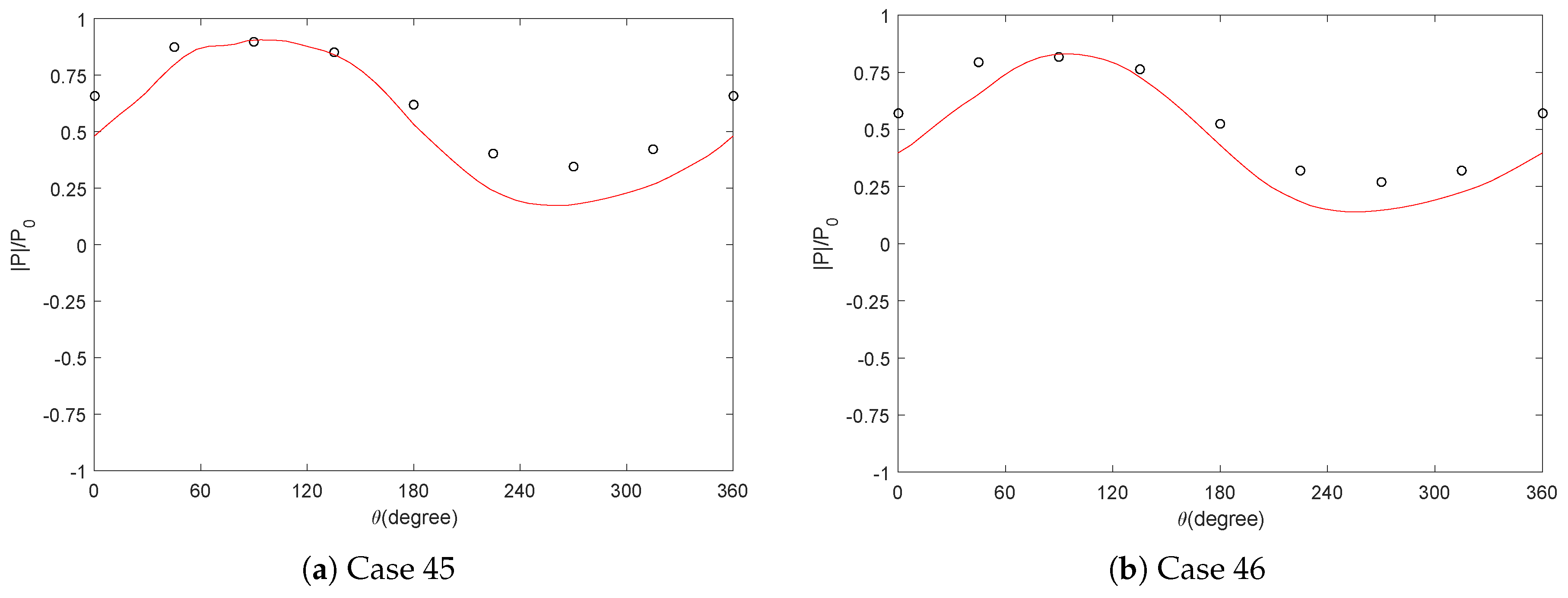
3.3. Comparison with Experimental Data for Wave-Induced Soil Response Around a Pipeline Buried in a Trench

The third validation is to compare the model with experimental data [40] for the case of a homogeneous seabed, in which the pipeline is in a trench. Stoke II wave loading simulated with OpenFoam is employed in this case. Sun et al. [40] conducted a series of laboratory experiments to examine the wave-induced pore-water pressure along the surface of a pipeline partially backfilled in a trench, and for brevity of presentation, only two typical comparisons are shown in this section in which the wave and seabed conditions are listed in Table 2 and Table 3. The corresponding comparisons of wave-induced pore pressure around the pipeline are illustrated in Figure 6. Red lines denote present numerical results and circle denote experimental data. It can be observed that the present numerical model agrees well with the laboratory experiments.

4. Results and Discussion

The aim of this study is to investigate the wave-pipeline-seabed interactions around a trenched pipeline by employing the proposed time-dependent meshless seabed model. In this section, the influence of soil properties, wave characteristics, and pipe configuration on the wave-induced oscillatory liquefaction are examined. Zen and Yamazaki [53] introduced and verified the concept of “oscillatory” excess pore pressure by conducting a series of experiments, and their criterion to determine the soil oscillatory liquefaction is used in this study, which can be expressed as
σ 0 ( z , 0 ) u e ( z , t ) = [ p ( 0 , t ) p ( z , t ) ]
where σ 0 ( z , 0 ) is the initial effective stress, and u e ( z , t ) = [ p ( 0 , t ) p ( z , t ) ] means the excess pore pressure. p ( 0 , t ) and p ( z , t ) denote the wave pressure at seabed surface and wave-induced pore pressure, respectively.
As shown in Figure 1, the pipeline is buried in the partially backfilled trench, and the lateral boundaries are considered as impermeable in this case. The direction of wave propagates along the positive x-direction. The Stokes II wave loading is simulated by OpenFOAM. Wave and soil parameters are listed in Table 4. When the effect of one parameter for the wave-induced pore pressure is examined, values of other parameters are kept fixed.

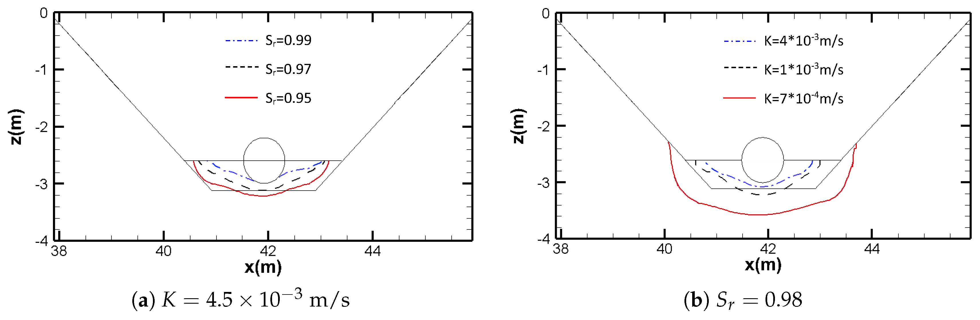
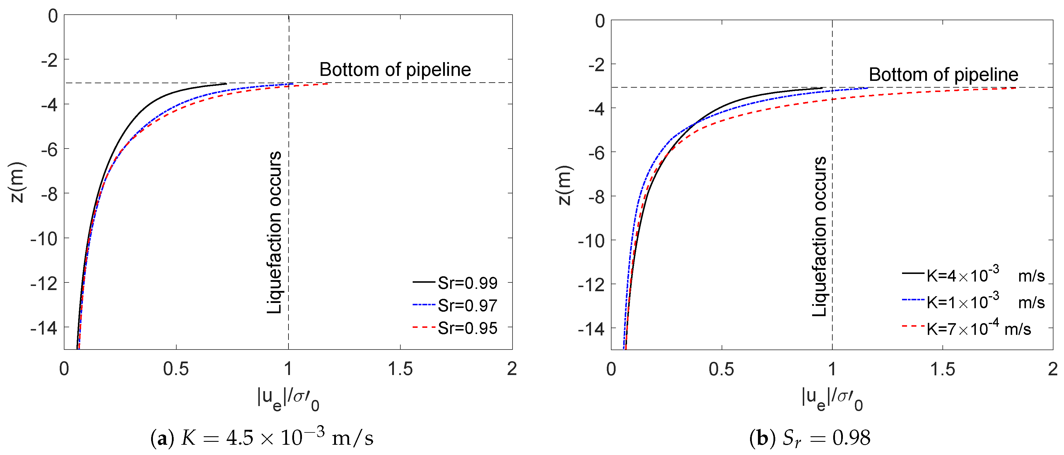
4.1. Effects of Soil Characteristics

Soil characteristics are significant factors to affect the wave-induced oscillatory soil response in the vicinity of a partially buried pipeline. In this section, two parameters are examined in detail. They are the degree of saturation S r and soil permeability K. Figure 7 presents the distribution of liquefaction depth around pipeline in the trench under various soil conditions, and Figure 8 shows the distributions of the maximum excess pore pressures under wave trough in the vertical section through the center of the pipeline. For Figure 7a and Figure 8a, permeability is 4 . 5 × 10 3 m/s. For Figure 7b and Figure 8b, degree of saturation is 0.98. Soil properties of backfills are chosen as same as bottom soil.
Three typical values of degree of saturation are considered in this section, they are: 95%, 97% and 99%, respectively. Figure 7a demonstrates that degree of saturation ( S r ) significantly affects the liquefaction depth in the trench. The depth is deeper with decreasing degree of saturation. Furthermore, from Figure 8a, it can be found that the soil on the bottom of the pipeline is much easier to be liquefied when degree of saturation is relatively small.
To investigate the influence of soil permeability on the wave-induced soil response, Figure 7b illustrates the distribution of the liquefaction depth in the trench with variable value of permeability, 4 × 10 3 m/s, 1 × 10 3 m/s and 7 × 10 4 m/s, respectively. Figure 8b shows the distribution of the maximum excess pore pressure under wave trough along the vertical section through the center of pipeline with variable permeability. It can be concluded that the liquefaction depth become large with decreasing permeability, and soil around the impermeable pipeline is much easier to be liquefied when permeability is relatively small.

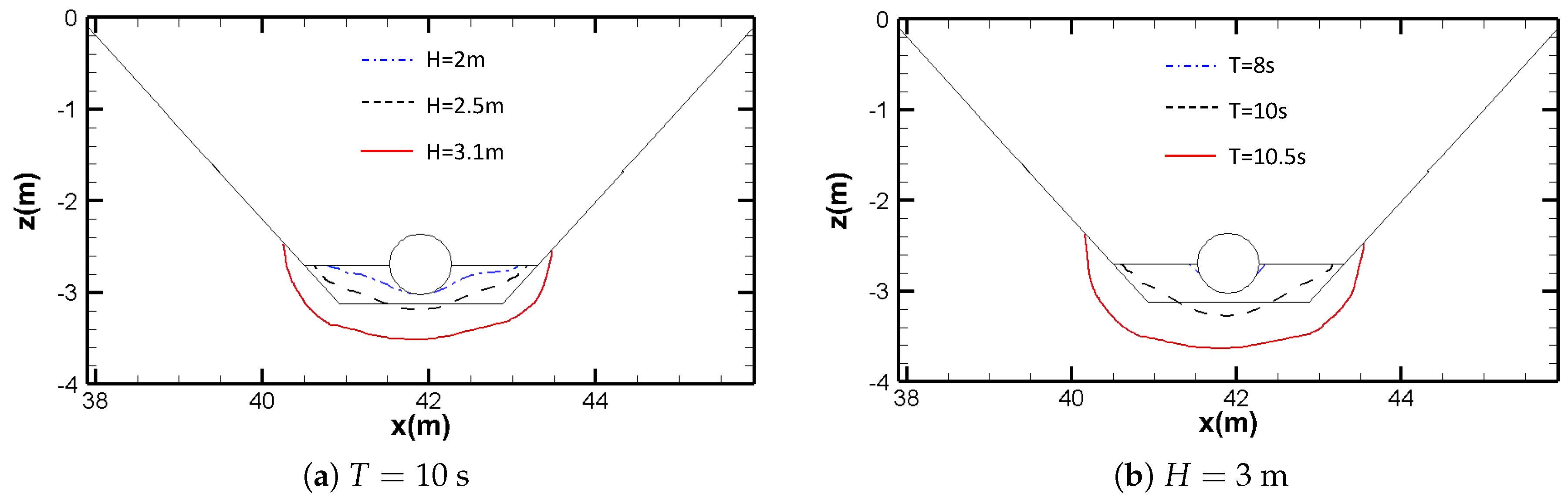
4.2. Effects of Wave Characteristics

In addition to soil characteristics, wave parameters have been found to significantly influence the wave-pipeline-seabed interactions. The influences of two wave parameters, wave height (H) and period (T), are examined in this section. The wave height H can directly affect the magnitude of wave loading exerting on the seabed surface. Wave period T affects the wave-induced oscillatory excess pore pressure by affecting wavelength. Figure 9 illustrates the distribution of oscillatory liquefaction depth in the trench under various wave height (H) and period (T), and the wave period is 10 s for Figure 9a, the wave height (H) is 3 m for Figure 9b. Figure 10 shows the distribution of the maximum excess pore pressure | u e | / σ 0 along the vertical section under the center of the pipeline.
Three values of wave height are examined in this section: 2 m, 2.5 m and 3.1 m. From Figure 9a, it can be found that the liquefaction depth increases with increasing wave height. Meanwhile, from Figure 10a, it can be seen that soil under the pipeline is much easier to be liquefied when wave height is relatively large.
Figure 9b and Figure 10b present the effect of wave period on the wave-induced oscillatory excess pore pressure around the trenched pipeline. Liquefaction depth from the seabed surface increases when wave period increases, and the soil on the bottom of pipeline is much easier to be liquefied when wave period is large.

4.3. Effects of Backfill

In this section, the effect of backfill depth ( H b ) on the wave-induced oscillatory liquefaction around a pipeline buried in a trench under the Stokes II wave loading is investigated. Three variable backfill depth are examined: 0.3 m, 0.5 m and 0.9 m. Figure 11 depicts the distribution of oscillatory liquefaction depth around the partially buried pipeline in a trench for various backfill depths, and Figure 12 illustrates the distribution of oscillatory excess pore pressure of the vertical section on the bottom of the pipeline under wave trough for the same four backfill depths. Figure 11 demonstrates that the liquefaction depth is greater with decreasing backfill depth. Similarly, from Figure 12, it can be seen that the maximum excess pore pressure increases as the backfill depth decreases.

5. Conclusions

This study proposes a two-dimensional seabed model by LRBFCM to investigate the wave-induced oscillatory liquefaction around a partially buried pipeline in a trench under non-linear wave loading. The model is validated by comparison with analytical solution, experimental data, and previous numerical results. The effects of wave characteristics, soil properties, and backfill depth in the trench are examined. The following conclusions can be drawn:
(1)
Unlike previous investigations using conventional numerical methods, this study established a meshless seabed model by employing LRBFCM and applied it to examine the wave-induced soil response. The validation with the analytical solution [38] and experimental data [39,40] shows that present model is satisfactory.
(2)
The wave-induced oscillatory excess pore pressure is relatively susceptible to the adjustment of degree of saturation ( S r ) and permeability (K) of soil. Low values of S r and K lead to great magnitude of wave-induced excess pore pressure around the pipeline.
(3)
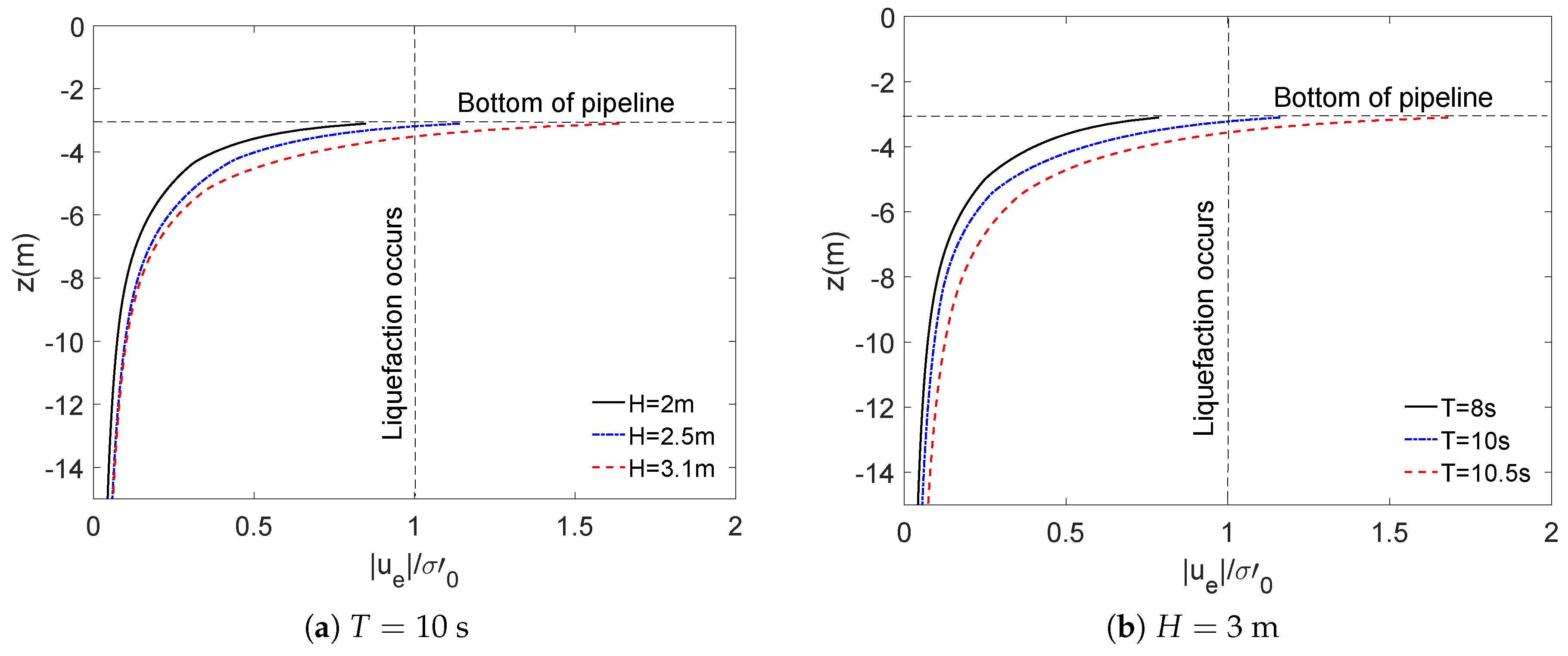
Oscillatory liquefaction depth is influenced significantly by wave characteristics, such as wave height (H) and wave period (T). Figure 9 shows that the liquefaction depth is deeper with increasing wave height (H) and wave period (T).
(4)
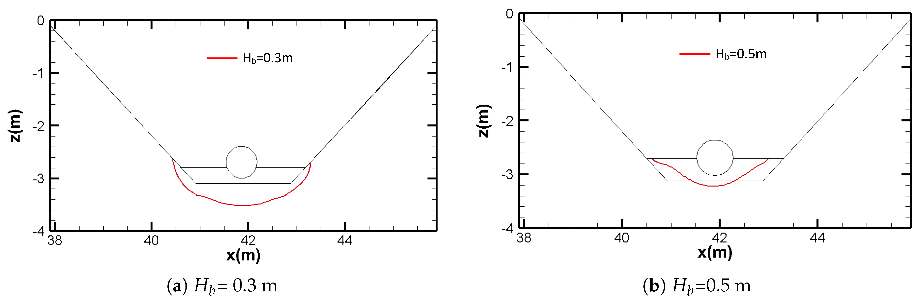
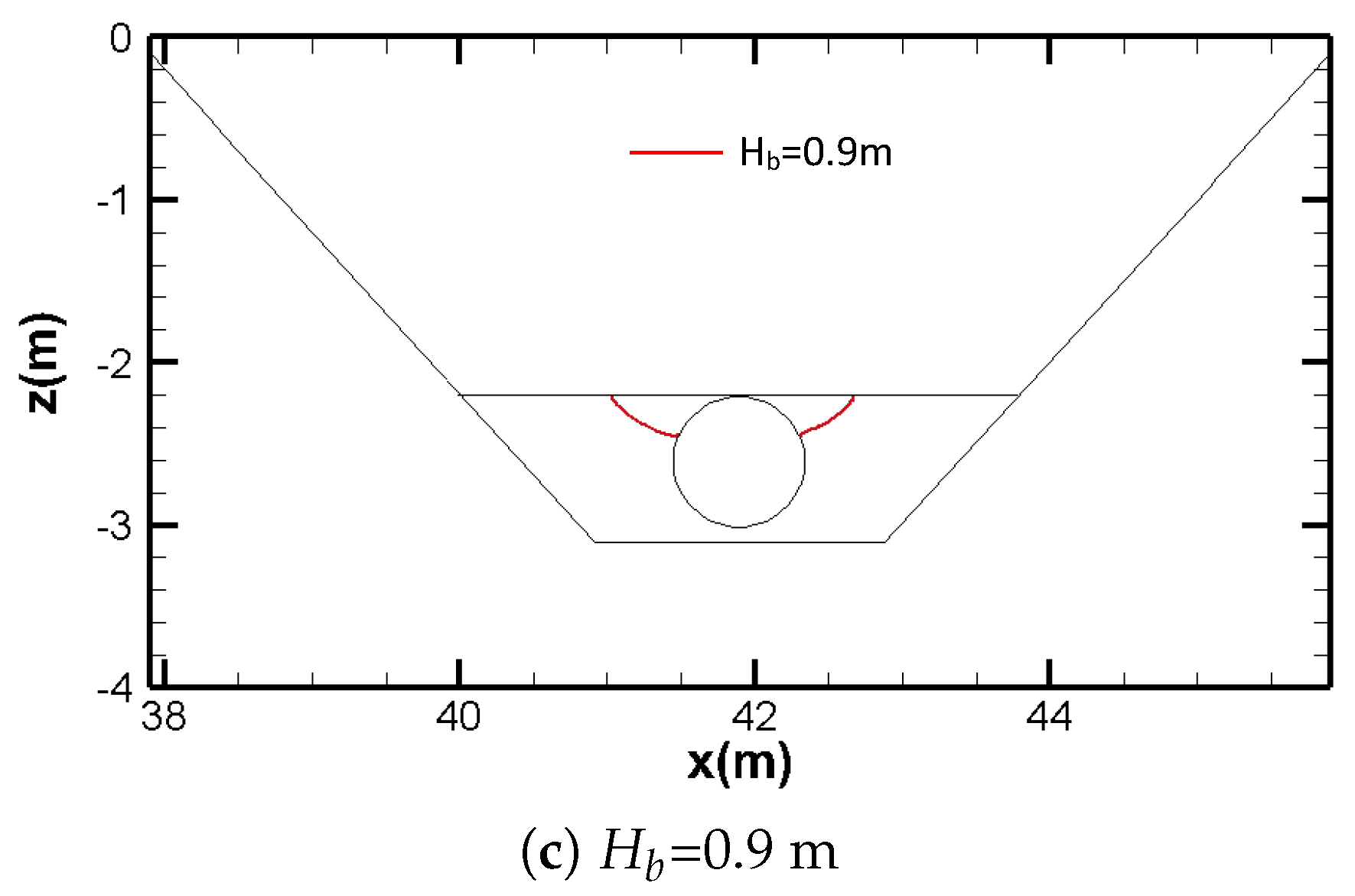
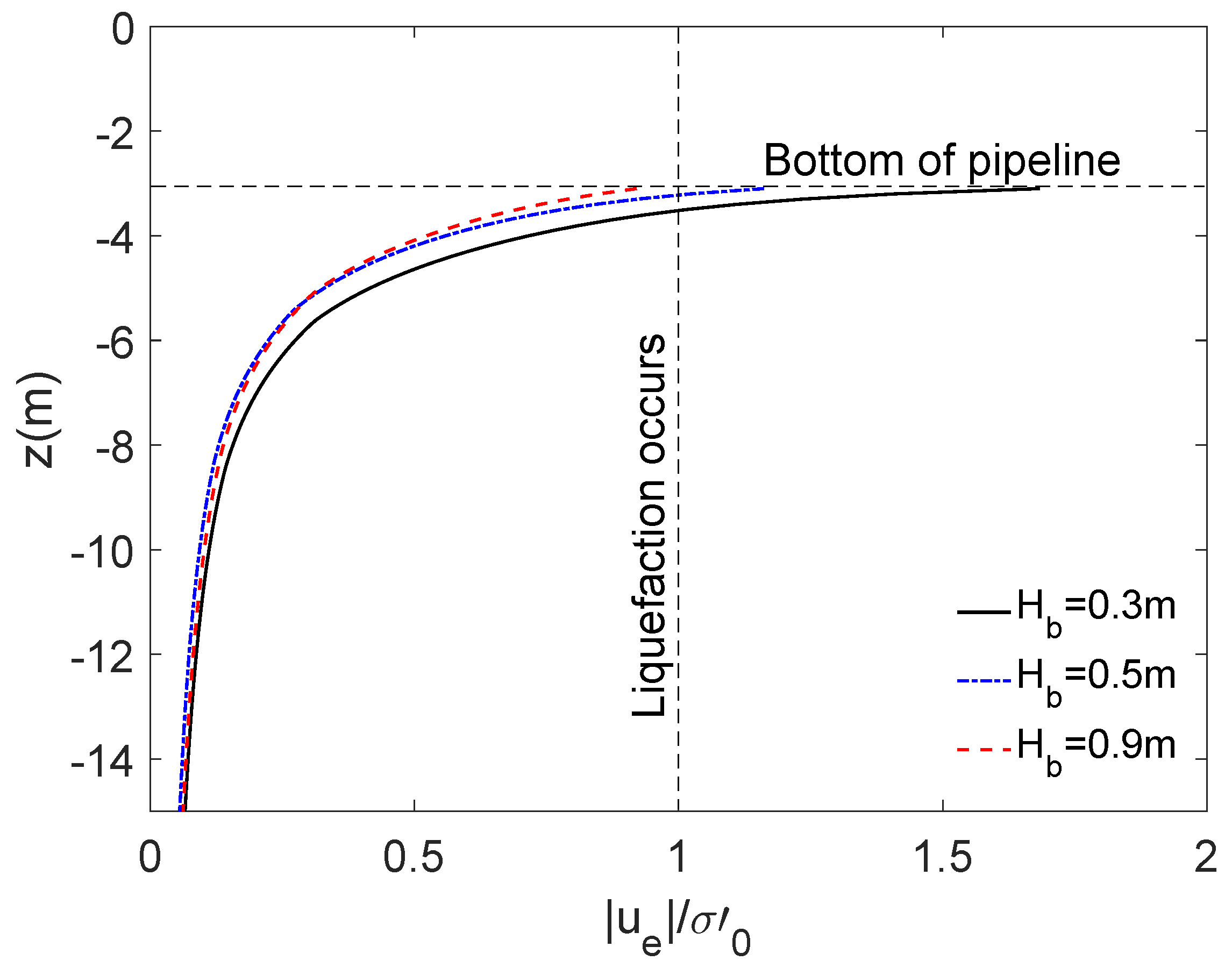
Pipe configuration is significantly important for the analysis of wave-pipeline-seabed interaction. In the process of increasing buried depth of pipe, the magnitude of oscillatory excess pore pressure at the bottom of the trenched pipeline decreases, which means that relatively large value of backfill depth can reduce the risk of liquefaction.
When the conventional methods with meshes are applied to analyze the computational domain with irregular boundaries, the elements or meshes may be distorted. Interpolation and re-meshing can be used to solve this problem. However, it requires more intensive work for complicated engineering problems. The meshless model presented in this study is designed for avoiding the poor mesh quality existing in conventional models. However, it needs to be further developed for different engineering problems if a huge number of nodes are required.
This study focuses on the wave-induced soil response under wave loading in two-dimensional. However, in real ocean environments, waves may approach the pipeline from any direction. Therefore, the effect of wave oblique on the soil response in the vicinity of pipelines will be examined in the future.

Author Contributions

Conceptualization, D.-S.J.; methodology, C.-C.T. & X.X.W., validation, X.X.W.; formal analysis, X.X.W.; writing—original draft preparation, X.X.W.; writing—review and editing, D.-S.J. & C.-C.T.; supervision, D.-S.J. & C.-C.T.

Funding

This research received funding from the Ministry of Science and Technology of Taiwan under the grant no. MOST 106-2918-I-022-001.

Acknowledgments

The authors are grateful for Miss K Sun at Hohai University (China) kindly providing her experimental data for the validation of the present model. The first author is grateful for the support of High-Performance Computing Cluster “Gowanda” to complete this research, and the support of scholarship from Griffith University. The third author is grateful for the support of the Ministry of Science and Technology of Taiwan under the grant no. MOST 106-2918-I-022-001.

Conflicts of Interest

The authors declare no conflict of interest.

References

  1. Christian, J.T.; Taylor, P.K.; Yen, J.K.C.; Erali, D.R. Large diameter underwater pipeline for nuclear power plant designed against soil liquefaction. In Proceedings of the Offshore Technology Conference, Houston, TX, USA, 6–8 May 1974; pp. 597–606. [Google Scholar]
  2. Clukey, E.C.; Vermersch, J.A.; Koch, S.P.; Lamb, W.C. Natural densification by wave action of sand surrounding a buried offshore pipeline. In Proceedings of the 21st Annual Offshore Technology Conference, Houston, TX, USA, 1–4 May 1989; pp. 291–300. [Google Scholar]
  3. Fredsøe, J. Pipeline-seabed interaction. J. Waterw. Port Coast. Ocean Eng. ASCE 2016, 142, 03116002. [Google Scholar] [CrossRef]
  4. Zen, K.; Yamazaki, H. Field observation and analysis of wave-induced liquefaction in seabed. Soils Found. 1991, 31, 161–179. [Google Scholar] [CrossRef]
  5. Seed, H.B.; Rahman, M.S. Wave-induced pore pressure in relation to ocean floor stability of cohesionless soils. Mar. Geotechnol. 1978, 3, 123–150. [Google Scholar] [CrossRef]
  6. Yamamoto, T.; Koning, H.; Sellmeijer, H.; Hijum, E.V. On the response of a poro-elastic bed to water waves. J. Fluid Mech. 1978, 87, 193–206. [Google Scholar] [CrossRef]
  7. Cheng, A.H.D.; Liu, P.L.F. Seepage force on a pipeline buried in a poroelastic seabed under wave loading. Appl. Ocean Res. 1986, 8, 22–32. [Google Scholar] [CrossRef]
  8. Thomas, S.D. A finite element model for the analysis of wave induced stresses, displacements and pore pressure in an unsaturated seabed. II: Model verification. Comput. Geotech. 1995, 17, 107–132. [Google Scholar] [CrossRef]
  9. Thomas, S.D. A finite element model for the analysis of wave induced stresses, displacements and pore pressure in an unsaturated seabed. I: Theory. Comput. Geotech. 1989, 8, 1–38. [Google Scholar] [CrossRef]
  10. Jeng, D.S.; Lin, Y.S. Finite element modelling for water waves–soil interaction. Soil Dyn. Earthq. Eng. 1996, 15, 283–300. [Google Scholar] [CrossRef]
  11. Jeng, D.S.; Lin, Y.S. Non-linear wave-induced response of porous seabed: A finite element analysis. Int. J. Numer. Anal. Methods Geomech. 1997, 21, 15–42. [Google Scholar] [CrossRef]
  12. Madga, W. Wave-induced uplift force acting on a submarine buried pipeline: Finite element formulation and verification of computations. Comput. Geotech. 1996, 19, 47–73. [Google Scholar]
  13. Madga, W. Wave-induced uplift force on a submarine pipeline buried in a compressible seabed. Ocean Eng. 1997, 24, 551–576. [Google Scholar]
  14. Madga, W. Wave-induced cyclic pore-pressure perturbation effects in hydrodynamic uplift force acting on submarine pipeline buried in seabed sediments. Coast. Eng. 2000, 39, 243–272. [Google Scholar]
  15. Jeng, D.S.; Lin, Y.S. Response of in-homogeneous seabed around buried pipeline under ocean waves. J. Eng. Mech. Eng. ASCE 2000, 126, 321–332. [Google Scholar] [CrossRef]
  16. Luan, M.; Qu, P.; Jeng, D.S.; Guo, Y.; Yang, Q. Dynamic response of a porous seabed-pipeline interaction under wave loading: Soil-pipe contact effects and inertial effects. Comput. Geotech. 2008, 35, 173–186. [Google Scholar] [CrossRef]
  17. Wen, F.; Jeng, D.S.; Wang, J.H. Numerical modeling of response of a saturated porous seabed around an offshore pipeline considering non-linear wave and current interactions. Appl. Ocean Res. 2012, 35, 25–37. [Google Scholar] [CrossRef]
  18. Zhao, H.; Jeng, D.S.; Guo, Z.; Zhang, J.S. Two-dimensional model for pore pressure accumulations in the vicinity of a buried pipeline. J. Offshore Mech. Arct. Eng. ASME 2014, 136, 042001. [Google Scholar] [CrossRef]
  19. Zhao, H.Y.; Jeng, D.S. Accumulation of pore pressures around a submarine pipeline buried in a trench layer with partially backfills. J. Eng. Mech. ASCE 2016, 142, 04016042. [Google Scholar] [CrossRef]
  20. Duan, L.L.; Liao, C.C.; Jeng, D.S.; Chen, L.Y. 2D numerical study of wave and current-induced oscillatory non-cohesive soil liquefaction around a parrtially buried pipeline in a trench. Ocean Eng. 2017, 135, 39–51. [Google Scholar] [CrossRef]
  21. Gingold, R.A.; Joseph, J.M. Smoothed particle hydrodynamics: Theory and application to non-spherical stars. Mon. Not. R. Astron. Soc. 1977, 181, 375–389. [Google Scholar] [CrossRef]
  22. Lucy, L.B. A numerical approach to the testing of the fission hypothesis. Astron. J. 1977, 82, 1013–1024. [Google Scholar] [CrossRef]
  23. Randles, P.W.; Libersky, L.D. Smoothed particle hydrodynamics: Some recent improvements and applications. Comput. Methods Appl. Mech. Eng. 1996, 139, 375–408. [Google Scholar] [CrossRef]
  24. Karim, M.R.; Nogami, T.; Wang, J.G. Analysis of transient response of saturated porous elastic soil under cyclic loading using element-free Galerkin method. Int. J. Solids Struct. 2002, 39, 6011–6033. [Google Scholar] [CrossRef] [Green Version]
  25. Wang, J.; Liu, G.; Lin, P. Numerical analysis of biot’s consolidation process by radial point interpolation method. Int. J. Solids Struct. 2002, 39, 1557–1573. [Google Scholar] [CrossRef]
  26. Wang, J.; Liu, G. A point interpolation meshless method based on radial basis functions. Int. J. Numer. Methods Eng. 2002, 54, 1623–1648. [Google Scholar] [CrossRef]
  27. Wang, J.G.; Zhang, B.; Nogami, T. Wave-induced seabed response analysis by radial point interpolation meshless method. Ocean Eng. 2004, 31, 21–42. [Google Scholar] [CrossRef]
  28. Kansa, E.J. Multiquadrics—A scattered data approximation scheme with applications to computational fluid-dynamics—I Surface approximations and partial derivative estimates. Comput. Math. Appl. 1990, 19, 127–145. [Google Scholar] [CrossRef]
  29. Kansa, E.J. Multiquadrics—A scattered data approximation scheme with applications to computational fluid-dynamics—II solutions to parabolic. Comput. Math. Appl. 2008, 19, 147–161. [Google Scholar] [CrossRef]
  30. Fasshauer, G.E. Solving partial differential equations by collocation with radial basis functions. In Proceedings of the Chamonix; Vanderbilt University Press: Nashville, TN, USA, 1996; Volume 1997, pp. 1–8. [Google Scholar]
  31. Mai-Duy, N.; Tran-Cong, T. Indirect RBFN method with thin plate splines for numerical solution of differential equations. Comput. Model. Eng. Sci. 2003, 4, 85–102. [Google Scholar]
  32. Šarler, B. A radial basis function collocation approach in computational fluid dynamics. Comput. Model. Eng. Sci. 2005, 7, 185–193. [Google Scholar]
  33. Lee, C.K.; Liu, X.; Fan, S.C. Local multiquadric approximation for solving boundary value problems. Comput. Mech. 2003, 30, 396–409. [Google Scholar] [CrossRef]
  34. Hardy, R.L. Multiquadric equations of topography and other irregular surfaces. J. Geophys. Res. 1971, 76, 1905–1915. [Google Scholar] [CrossRef]
  35. Šarler, B.; Vertnik, R. Meshfree explicit local radial basis function collocation method for diffusion problems. Comput. Math. Appl. 2006, 51, 1269–1282. [Google Scholar] [CrossRef] [Green Version]
  36. Kosec, G.; Sarler, B. Local RBF collocation method for Darcy flow. Comput. Model. Eng. Sci. 2008, 25, 197–208. [Google Scholar]
  37. Tsai, C.C.; Lin, Z.H.; Hsu, T.W. Using a local radial basis function collocation method to approximate radiation boundary conditions. Ocean Eng. 2015, 105, 231–241. [Google Scholar] [CrossRef]
  38. Hsu, J.R.C.; Jeng, D.S. Wave-induced soil response in an unsaturated anisotropic seabed of finite thickness. Int. J. Numer. Anal. Methods Geomech. 1994, 18, 785–807. [Google Scholar] [CrossRef]
  39. Turcotte, B.R.; Liu, P.L.F.; Kulhawy, F.H. Laboratory Evaluation of Wave Tank Parameters for Wave-Sediment Interaction; Technical Report; Joseph F. Defree Hydraulic Laboratory, School of Civil and Environmental Engineering, Cornell University: Ithaca, NY, USA, 1984. [Google Scholar]
  40. Sun, K.; Zhang, J.S.; Guo, Y.; Jeng, D.S.; Guo, Y.K.; Liang, Z.D. Ocean waves propagating over a partially buried pipeline in a trench layer: Experimental study. Ocean Eng. 2019, 173, 617–627. [Google Scholar] [CrossRef]
  41. Jeng, D.S.; Zhao, H.Y. Two-dimensional model for pore pressure accumulations in marine sediments. J. Waterw. Port Coast. Ocean Eng. ASCE 2015, 141, 04014042. [Google Scholar] [CrossRef]
  42. Higuera, P.; Lara, J.L.; Losada, I.J. Simulating coastal engineering processes with OpenFOAM. Coast. Eng. 2013, 71, 119–134. [Google Scholar] [CrossRef]
  43. Higuera, P.; Lara, J.L.; Losada, I.J. Realistic wave generation and active wave absorption for Navier-Stokes models: Application to OpenFOAM. Coast. Eng. 2013, 71, 102–118. [Google Scholar] [CrossRef]
  44. Higuera, P.; Lara, J.L.; Losada, I.J. Three-dimensional interaction of waves and porous coastal structures using OpenFOAM. Part I: Formulation and validation. Coast. Eng. 2014, 83, 243–258. [Google Scholar] [CrossRef]
  45. Higuera, P.; Lara, J.L.; Losada, I.J. Three-dimensional numerical wave generation with moving boundaries. Coast. Eng. 2015, 101, 35–47. [Google Scholar] [CrossRef]
  46. Jeng, D.S.; Rahman, M.S.; Lee, T.L. Effects of inertia forces on wave-induced seabed response. Int. J. Offshore Polar Eng. 1999, 9, 307–313. [Google Scholar]
  47. Biot, M.A. General theory of three-dimensional consolidation. J. Appl. Phys. 1941, 26, 155–164. [Google Scholar] [CrossRef]
  48. Bentley, J.L. Multidimensional binary search trees used for associative searchings. Commun. ACM 19752, 18, 509–517. [Google Scholar] [CrossRef]
  49. Liu, X.; Liu, G.; Tai, K.; Lam, K. Radial point interpolation collocation method (rpicm) for partial differential equations. Comput. Math. Appl. 2005, 50, 1425–1442. [Google Scholar] [CrossRef]
  50. Jeng, D.S.; Cha, D.H.; Lin, Y.S.; Hu, P.S. Analysis on pore pressure in an anisotropic seabed in the vicinity of a caisson. Appl. Ocean Res. 2000, 22, 317–329. [Google Scholar] [CrossRef]
  51. Zienkiewicz, O.C.; Scott, F.C. On the principle of repeatability and its application in analysis of turbine and pump impellers. Int. J. Numer. Methods Eng. 1972, 9, 445–452. [Google Scholar] [CrossRef]
  52. Ye, J.; Jeng, D.S. Response of seabed to natural loading-waves and currents. J. Eng. Mech. ASCE 2012, 138, 601–613. [Google Scholar] [CrossRef]
  53. Zen, K.; Yamazaki, H. Mechanism of wave-induced liquefaction and densification in seabed. Soils Found. 1990, 30, 90–104. [Google Scholar] [CrossRef]
Figure 1. Sketch for wave-seabed-pipeline interactions.
Jmse 07 00087 g001
Figure 2. Comparison of wave-induced seabed response between the cases with periodic and fixed lateral boundaries.
Jmse 07 00087 g002
Figure 3. The wave-induced pore pressure in the vicinity of pipeline with various node number, c and K ¯ .
Jmse 07 00087 g003
Figure 4. Comparison of the vertical distribution of pore pressure ( | p | / p 0 ) and stresses ( | σ x | / p 0 , | σ z | / p 0 and | τ x z | / p 0 ) versus z / h between the present model (the solid lines) and analytical solutions [38] (symbols).
Jmse 07 00087 g004
Figure 5. The wave-induced pore pressure in the vicinity of a fully buried pipeline. (red dashed line: numerical results of Cheng and Liu [7]; blue star: FEM results by COMSOL model [41]; circle line: experimental data [39]; solid line: present results).
Jmse 07 00087 g005
Figure 6. Distribution of wave-induced pore pressure around a trenched pipeline (red solid line: the present result; circle: experimental data [40]).
Jmse 07 00087 g006
Figure 7. Distribution of the liquefaction depth around the partially buried pipeline for variable degree of saturation and permeability.
Jmse 07 00087 g007
Figure 8. Distribution of the excess pore pressure ( | u e | / σ 0 ) under wave trough along the vertical section through the center of the pipeline for different soil properties.
Jmse 07 00087 g008
Figure 9. Distribution of the liquefaction depth around the partially buried pipeline for variable wave height and period.
Jmse 07 00087 g009
Figure 10. Distribution of the excess pore pressure ( | u e | / σ 0 ) under wave trough along the vertical section through the center of the pipeline for various wave characteristics.
Jmse 07 00087 g010
Figure 11. Distribution of the liquefaction depth around the partially buried pipeline for variable backfill depth.
Jmse 07 00087 g011aJmse 07 00087 g011b
Figure 12. Distribution of the excess pore pressure ( | u e | / σ 0 ) under wave trough along the vertical section through the center of the pipeline for various backfill depth.
Jmse 07 00087 g012
Table 1. Input data for numerical examples demonstrating effects of lateral boundary conditions.
Wave Characteristics
Wave period T 8.0 s
Water depth d 20 m
Wave length L 88.88 m
Soil Characteristics
Thickness of seabed h 30 m
Poisson’s ratio μ 0.33333
Soil porosity n 0.3
Soil permeability K 10 2 m/s
Degree of saturation S r 0.98
Shear modulus G 10 7 N/m 2
Table 2. Input data for the comparison with experimental data [40].
Wave Characteristics
Water depth d 0.4 m
Soil Characteristics
Thickness of seabed h 0.58 m
Poisson’s ratio μ 0.32
Soil porosity n 0.396
Soil permeability K 3.56 × 10 5 m/s
Degree of saturation S r 0.998
Geometry of the Pipe
Pipe radius R 0.05 m
Table 3. Wave and seabed conditions for the comparison with experimental data [40].
Case No.Wave ConditionSeabed Condition
Wave Height H (m)Wave Period T (s)Trench Depth (m)Backfill Depth (m)
450.121.60.150.1
460.121.60.150.125
Table 4. Input data for the parametric study.
Wave Characteristics
Wave period T 10 s
Water depth d 8 m
Wave height H 3 m
Soil Characteristics
Thickness of seabed h 30 m
Poisson’s ratio μ 0.35
Soil porosity n 0.425
Soil permeability K 1 × 10 3 m/s
Degree of saturation S r 0.98
Geometry of the Pipe
Pipe radius R 0.4 m
Backfilled depth H b 0.5 m

