Experimental Study and Estimation of Groundwater Fluctuation and Ground Settlement due to Dewatering in a Coastal Shallow Confined Aquifer

Abstract

The coastal micro-confined aquifer (MCA) in Shanghai is characterized by shallow burial depth, high artesian head, and discontinuous distribution. It has a significant influence on underground space development, especially where the MCA is directly connected with deep confined aquifers. In this paper, a series of pumping well tests were conducted in the MCA located in such area to investigate the dewatering-induced groundwater fluctuations and stratum deformation. In addition, a numerical method is proposed for the estimation of hydraulic parameter, and an empirical prediction method is developed for dewatering-induced ground settlement. Test results show that groundwater drawdowns and soil settlement can be observed not only in MCA but also in the aquifers underneath it. This indicates that there is a close hydraulic connection among each aquifer. Moreover, the distributions and development of soil settlement at various depths are parallel to those of groundwater drawdowns in most areas of the test site except the vicinity of pumping wells, where collapse-induced subsidence due to high-speed flow may occur. Furthermore, the largest deformation usually occurs at the top of the pumping aquifer instead of the ground surface, because the top layer is expanded due to the stress arch formed in it. Finally, the proposed methods are validated to be feasible according to the pumping well test results and can be employed to investigate the responses of groundwater fluctuations and stratum deformations due to dewatering in MCA.

1. Introduction

Shanghai is located at the riverfront and coastal plain of the Yangtze River deltaic deposit, where soft Quaternary deposits with a thickness of about 300 m are widely distributed [1,2]. In this region, an alternated multi-aquifer-aquitard system (MAAS) is formed due to complicated palaeoclimatic and palaeogeographic conditions as well as frequent transgressions and regressions in history [3,4,5]. The groundwater system in Shanghai is a part of the deltaic groundwater system of the Yangtze River [4] and mainly includes a phreatic aquifer group and five confined aquifers (labeled as Aq I to Aq V). Specifically, the phreatic aquifer group is composed of a phreatic aquifer (labeled as Aq0) and a micro-confined aquifer (labeled as MCA). All the aquifers are separated by seven aquitards (labeled as Ad0 to Ad VI). According to the distribution of MCA and its hydraulic connection with adjacent aquifers, the MAAS in Shanghai central city can be divided into five types (labeled as Type I to Type V), as depicted in Figure 1d. A geological survey shows that the MAAS keeps abundant and high artesian groundwater in aquifer layers [6], easily causing adverse effects on the construction of the underground facilities as well as deep excavations in these soft deposits [7,8,9,10], especially the groundwater stored in MCR, Aq I and Aq II. In past few decades, the influence of Aq I and Aq II has been deeply concerning and widely studied by both researchers and engineers [7,9,10,11,12,13], whereas literatures concentrated on the influence of MCA are rare.

The micro-confined aquifer in Shanghai is located at the top of MAAS and is the lower sublayer, underneath the phreatic aquifer, of Holocene phreatic aquifer group. The aquifer is discontinuously distributed in the horizon direction and is usually buried at a depth of only 15 to 22 m [4]. For this reason, the piezometric head of the groundwater in MCA is easily affected by meteorological and hydrological conditions [3] and periodically varies from 3 to 11 m below the ground surface [14,15]. The thickness of the aquifer generally varies from 5 to 20 m in most regions, whereas in the region of Type V, MCA is directly connected with Aq I due to the hiatus of Ad I and its thickness can reach 40 to 50 m [4,16,17]. Additionally, the MCA in Shanghai is mainly composed of silty sand and silty clay and its hydraulic conductivity is relatively lower than those of the deep confined aquifers. The hydraulic conductivity of MCA is variable between (3~6) × 10⁻⁵~10⁻³ cm/sec while those of Aq I and Aq II usually vary between (3~6) × 10⁻⁴~10⁻³ cm/sec and (2~6) × 10⁻³~10⁻² cm/sec, respectively [14]. In addition, the maximum specific discharge capacity of MCA is about 43.2 m³/day-meter, which is also smaller than those of deep confined aquifers with the maximum being greater than 720 m³/day-meter, e.g., Aq II and Aq IV [4].

As aforementioned, the artesian head in the MCA is high, and the burial depth of MCA is small, causing deep excavations to be more easily affected by the MCA, especially the MCA in Type V. Moreover, with rapid development of ocean economy and coastal industry in recent decades, an increasing number of municipal and commercial infrastructures, e.g., metro tunnels and stations, were or are being constructed in the coastal soft deposits of Shanghai [4,18,19,20,21], resulting in the increase of excavation scale and depth [5,22,23,24]. In some projects, the depth of excavation reaches the top of MCA [15]. As excavation depth is increased, the remaining bottom soil is insufficient to counteract the artesian head underneath the excavation, leading to seepage and inrushing damage to the excavation [9,25,26]. This is particularly true for the excavations above the coastal MCA, for which the critical excavation depth is usually less than 10 m according to the Shanghai design specification for the requirement of surge resistance [14]. Consequently, dewatering measurements should be adopted in excavations to reduce or even eliminate the adverse effects due to artesian groundwater [8,10,26,27,28].

However, regardless of many advantages of dewatering for protecting excavations, it has been widely accepted that groundwater extraction can induce stratum deformation in the vicinity of the excavations [5,7,8,18,19,29,30,31,32,33] as well as secondary hazards to surrounding structures [34,35,36,37]. Many scholars and engineers have been devoted to investigating the dewatering-induced environment influence in Shanghai. As a matter of fact, these studies were primarily concentrated on the influence of groundwater extraction in deep confined aquifers [10,11,12], such as Aq I and Aq II, whereas few literatures were dealt with that in the shallow-buried MCA. As above mentioned, the hydrological and geological conditions (e.g., burial depth, compressibility, hydraulic conductivity, and specific discharge capacity) of the MCA are distinguished from those of deep confined aquifers. Additionally, the MCA is more easily affected by meteorological and hydrological conditions than deep confined aquifers due to its shallow burial depth [3], resulting in complex hydrological conditions in the MCA. Moreover, hydrological conditions can be more complex if there is aquitard hiatus, e.g., in the MAAS of Type V, where the MCA is directly connected with Aq I due to the hiatus of Ad I. Considering these factors, the environmental risk from excavation dewatering in a coastal MCA is still uncertain.

The objective of this study is to investigate the response of groundwater fluctuations and ground settlement induced by dewatering in the coastal MCA of Shanghai. To achieve this aim, a series of field pumping well tests were conducted at a construction site located at Pudong New Area District, where the MCA is connected directly with Aq I. To help analyze the responses, the following are addressed:

• How are MCA and Aq I hydraulically connected and how does the hydraulic connection affect the responses of groundwater fluctuations and strata deformation?
• What is the correlation between stratum deformation (ground settlement, stratum compression) and groundwater fluctuations?
• How to estimate the hydrogeological parameters of the MCA based on pumping well tests if the MCA is directly connected with the confined aquifer.
• How to predict the ground settlement induced by dewatering in the MCA when the MCA is directly connected with the confined aquifer.

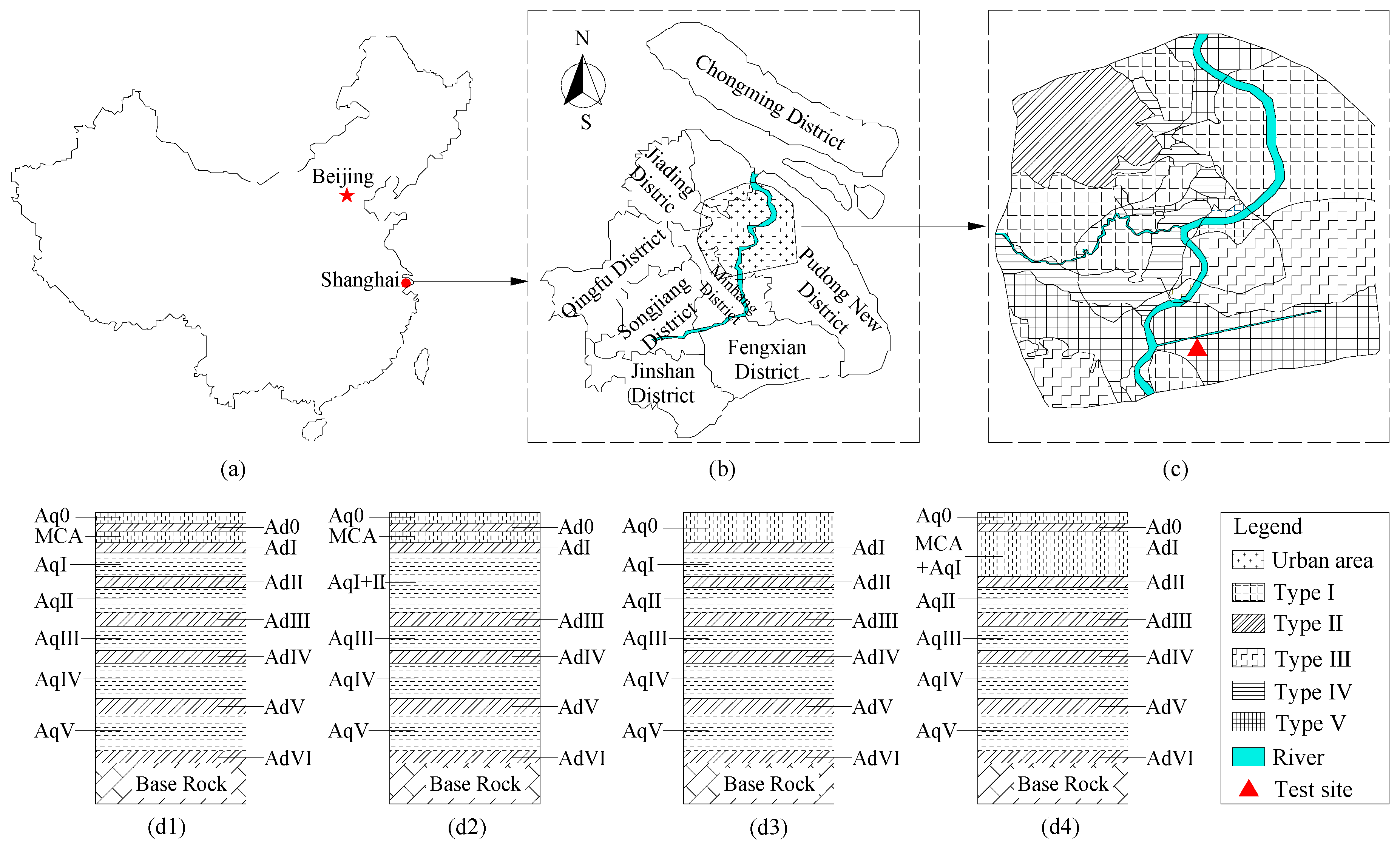
2. Study Area

To investigate the responses of groundwater fluctuations and stratum deformation as well as the influence on excavation, three groups of single-well pumping test and a group of multi-well pumping test were conducted.

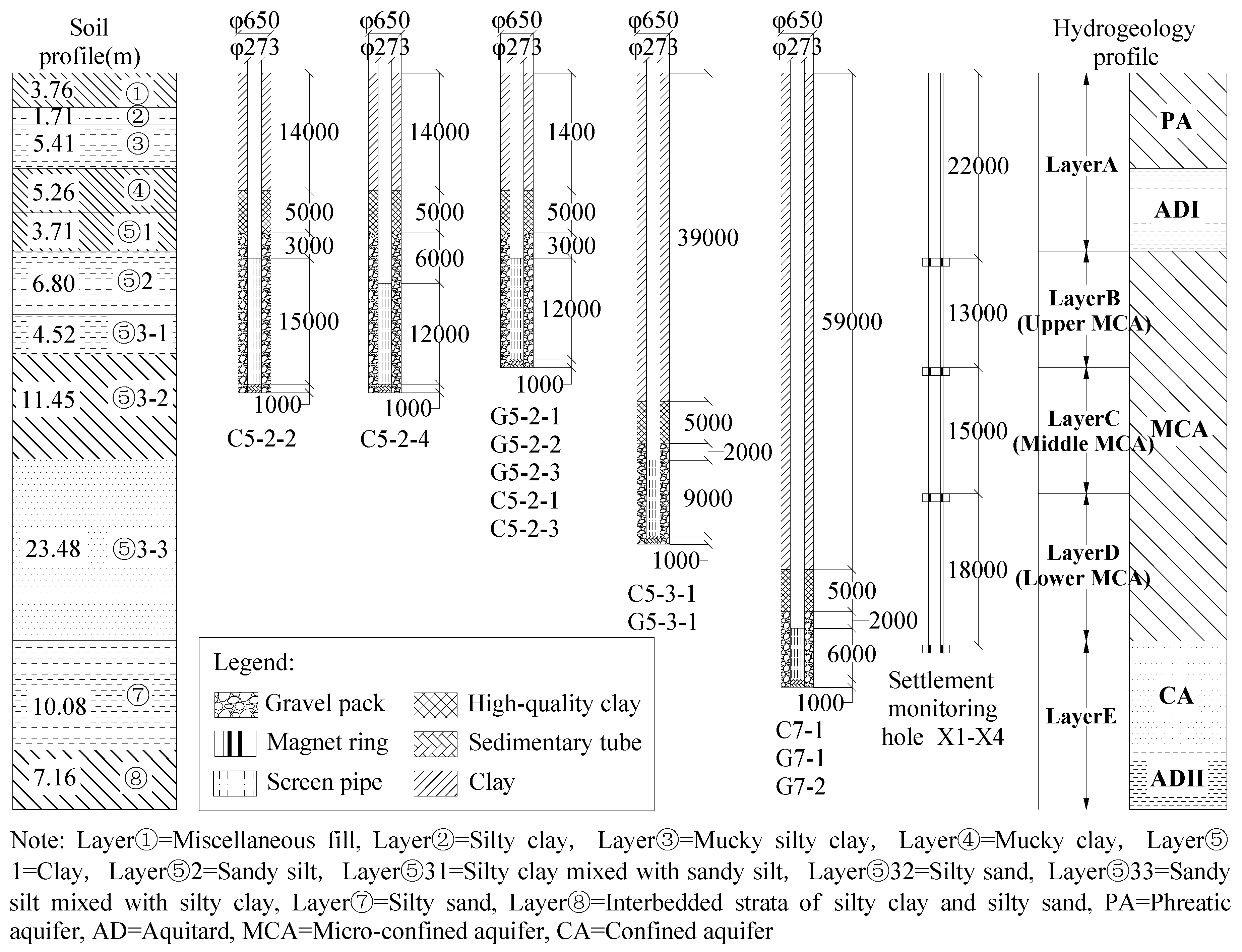
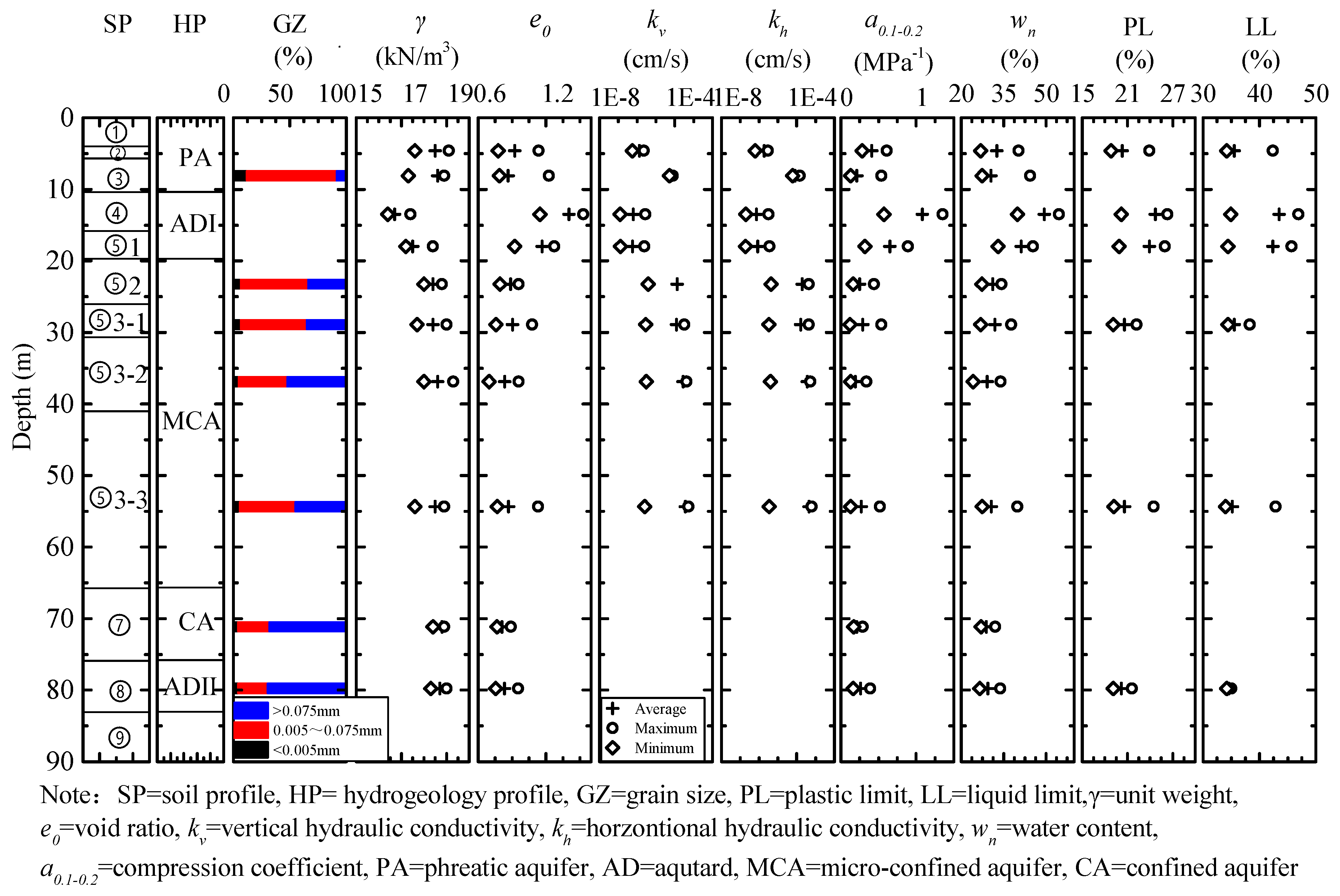
2.1. Engineering Geology

The test site is located in the northwest of Pudong New Area District (as shown in Figure 1c), and the elevation at the test site varies from 4.57 m to 5.66 m. The soil distributed in the influence depth of the foundation is characterized as a depositional soil layer of the coastal plain from Quaternary Holocene to Pleistocene, mainly including clay, silty soil, and silty sand. The columns in the left part Figure 2 plot the soil profile of the construction site. The first layer is an artificial layer in the upper about 3.76 m below the land surface, underlain by silty clay, mucky silty clay, mucky clay, and clay to the depth of about 19.85 m. The following layer is sandy silt to the depth of about 25.65 m overlying the layer of silty clayey silt to the depth of about 30.17 m. The next layer is a silt layer extending to a depth of about 41.42 m, followed by sandy silt mixed up with silty clay to a depth of about 64.90 m. Underneath the above layers is silty sand to a depth of about 74.98 m. Vertically below all these layers is the interbedded strata of silty clay and silty sand until the termination depth of about 82.14 m.

Figure 3 presents the geotechnical parameters for each layer at the test site. The grain size distribution indicates that the content of silty sand and sand in deep confined aquifers is higher than that in the MCR. The initial void ratio, $e_0$, was determined based on the physical properties of the soils at different depths tested from the laboratory tests. The vertical and horizontal hydraulic conductivity, $k_v$ and $k_h$, of soils were obtained based on laboratory tests and injection tests. The compression index, $a_{0.1-0.2}$, was determined by laboratory oedometer tests. The water content of each stratum was usually close to its liquid limit, whereas the plastic limit varied little along with the depth and was approximately 21%.

2.2. Hydrogeology

There are mainly three types of groundwater stored in the influence depth of the proposed project, and they are phreatic water referred to as phreatic aquifer, feeble confined water known as MCA, and confined water dubbed as confined aquifer (Aq I), respectively. As can be seen in Figure 2, the phreatic aquifer and the MCA are separated by an aquitard (Ad0) while MCA is adjacent to the confined aquifer directly and there is a certain hydraulic connection between the two aquifers. The phreatic aquifer is mainly composed of the silty clay with a thickness of about 9 m, and the water head of it is variable from 0.75 m to 1.70 m below the ground surface. The MCA is primarily stored in the sandy silt (Layer ⑤2), the silty sand (Layer ⑤3-2), and the silty clay (Layer ⑤3-3) with an aggregate thickness of about 44.2 m. The artesian head in these layers varies from −5.1 m to −6.8 m compared to the ground surface. In addition, the confined aquifer is mainly composed of silty sand (Layer ⑦) with a thickness of about 9.8 m and the water level varies from −8.9 m to −9.7 m.

3. Pumping Well Tests

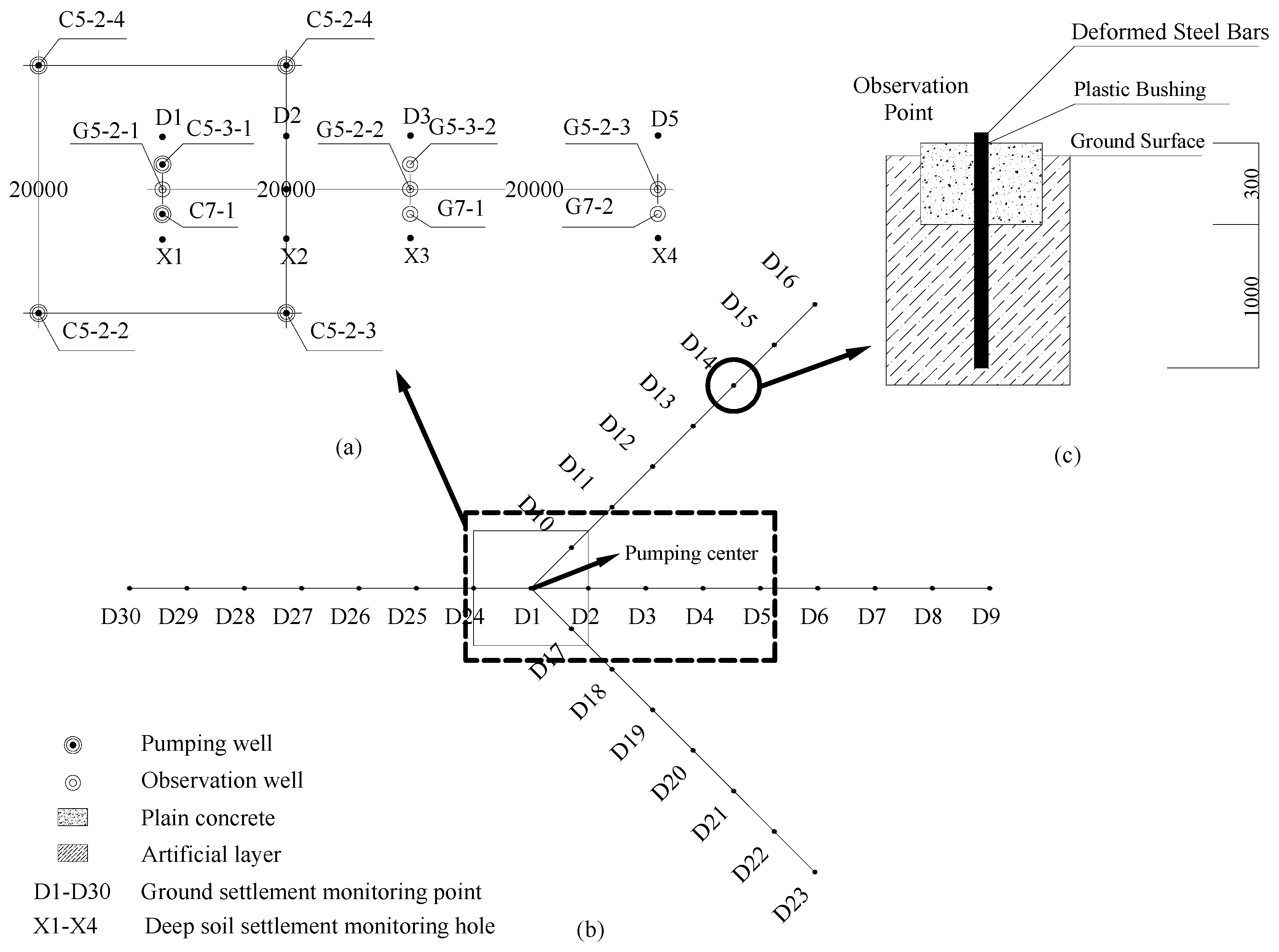
3.1. Well Installation

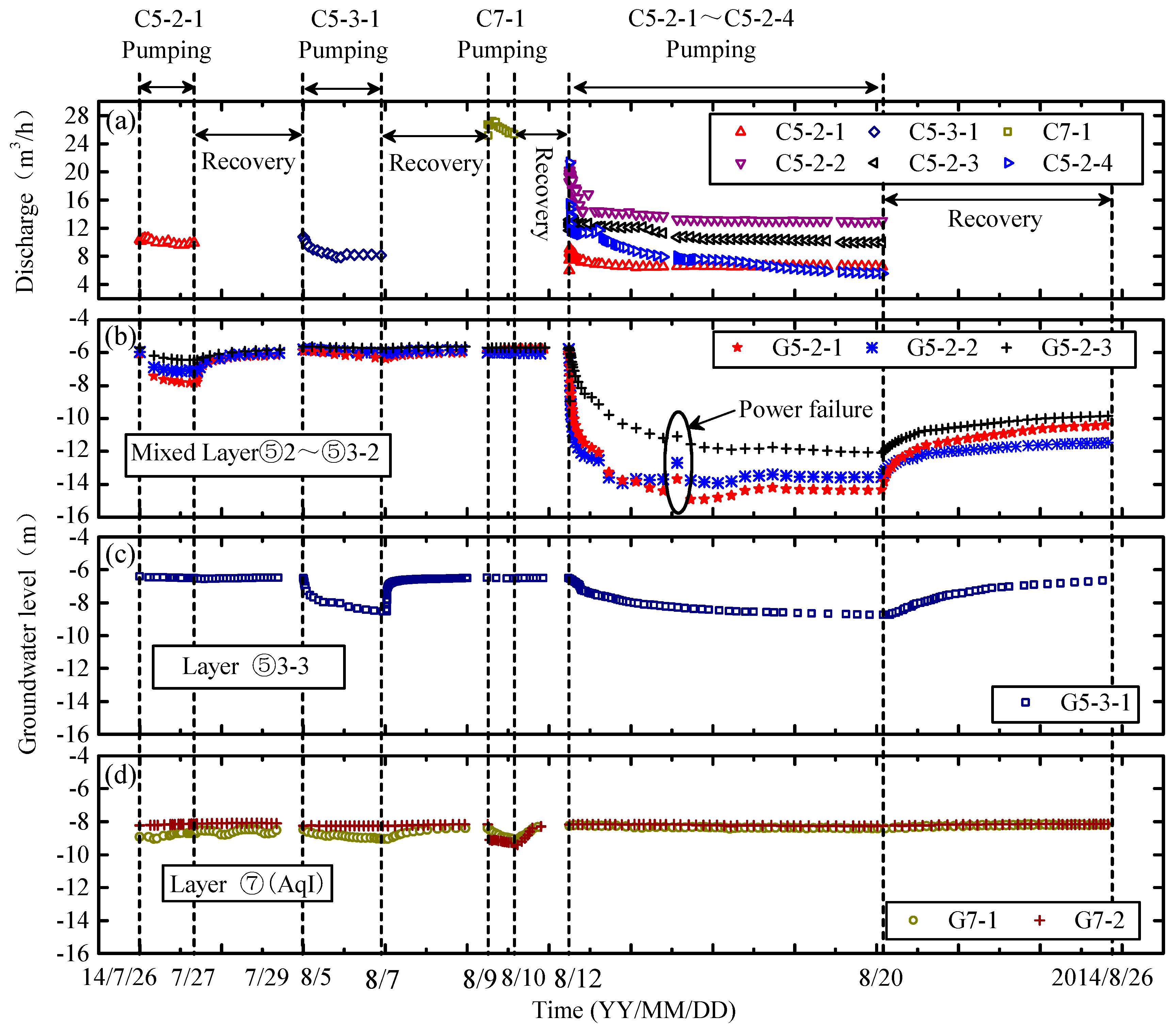
In the tests, twelve test wells, including seven pumping wells and five observation wells, were employed. The layout of the wells is plotted in Figure 4, and the distance between each well is also labeled in the figure. Each test well was composed of a steel tube, screen pipe, and sedimentary pipe. The steel pipe was installed at the upper part of a well and outside the steel pipe were sealed with clay, high-quality clay, and gravel pack from top-down to prevent the groundwater from the upper aquifers flowing into test wells. The screen was installed underneath the steel pipe and outside the screen was backfilled with gravel to ensure the groundwater flowed into the well smoothly. The sedimentary pipe with a length of 1 m was installed at the bottom of the well to prevent the screen pipe being clogging by the sediment in the groundwater. The structures of the test well are depicted in Figure 2, and the associated parameters are also presented in the figure.

In the tests, there were four pumping wells (labelled C5-2-1~C5-2-4, at a depth of 35 m, 38 m, 35 m, 38 m, respectively) and three observation wells (labelled G5-2-1~G5-2-3, at a depth of 35 m) installed in Layers ⑤2~⑤3-2, a pumping well (labelled C5-3-1, at a depth of 56 m) and an observation well (labelled G5-3-1, at a depth of 56 m) installed in Layer ⑤3-3, a pumping well (labelled C7-1, at a depth of 73 m) and two observation wells (labelled G7-1 and G7-2, at a depth of 73 m) installed in Layer ⑦. The detailed structural parameters for each well are listed in

Table 1. Detailed characteristics of test wells.

Well Type	Well Number	Buried Depth of Well Bottom (m)	Internal Diameter (mm)	External Diameter (mm)	Buried Depth of Well Screen (m)		Pumping/ Monitoring Stratum
					Upper	Bottom
Pumping well	C5-2-1	35	273	650	20	34	⑤2~⑤3-2
	C5-2-2	38	273	650	20	37	⑤2~⑤3-2
	C5-2-3	35	273	650	20	34	⑤2~⑤3-2
	C5-2-4	38	273	650	20	37	⑤2~⑤3-2
	C5-3-1	56	273	650	46	55	⑤3-3
	C7-1	73	273	650	66	72	⑦
Monitoring well	G5-2-1	35	168	650	22	34	⑤2~⑤3-2
	G5-2-2	35	168	650	22	34	⑤2~⑤3-2
	G5-2-3	35	168	650	22	34	⑤2~⑤3-2
	G5-3-1	56	168	650	46	55	⑤3-3
	G7-1	73	168	650	66	72	⑦
	G7-2	73	168	650	66	72	⑦

. The external radius for pumping well was identical to that for observation well and was 650 mm, whereas the internal radius for pumping well was 273 mm while that for observation well was 168 mm. The length of the screen for C5-2-1~C5-2-4 was 14 m, 17 m, 14 m, and 12 m, respectively, for G5-2-1~G5-2-3 it was 12 m, for C5-3-1 and G5-3-1 it was 9 m, for C7-1 and G7-1~G7-2 it was 6 m.

3.2. Test Scheme

Three single-well pumping tests and a multi-well pumping test were performed successively from July 26, 2014, to August 26, 2014.

Table 2. Process of the pumping well tests.

Test Type	Pumping Aquifer	Well Number	sw (m)	t0	te	tp (min)	tr (min)	Q (m3/h)
Single- well	⑤2~⑤3-2	C5-2-1	8.94	09:00 26 Jul.	18:37 27 Jul.	2017	2920	−9.96
	⑤3-3	C5-3-1	31.21	12:00 5 Aug.	13:00 7 Aug.	2940	2828	−9.77
	⑦	C7-1	10.21	08:00 9 Aug.	10:00 10 Aug.	980	1020	−26.7
Multi- well	⑤2~⑤3-2	C5-2-1	10.87	12:00 12 Aug.	15:00 20 Aug.	10930	8120	−7.28
		C5-2-2	7.82					−15.64
		C5-2-3	7.63					−11.68
		C5-2-4	9.69					−10.87

Note: $s_w$ = drawdown in pumping well; $t_0$ = start time; $t_e$ = end time; $t_p$ = pumping time; $t_r$ = recovery time; $Q$ = discharge rate.

shows the detailed process of the tests. The single-well pumping tests were performed in Layers ⑤2~⑤3-2 using well C5-2-1 at a rate of 9.96 m³/h from 9:00, July 26 to 18:37, July 27 lasting for 2017 min, in Layer ⑤3-3 using well C5-3-1 at a rate of 9.77 m³/h from 12:00, August 5 to 13:00, August 7 lasting for 2940 min and in Layer ⑦ using well C7-1 at a rate of 26.7 m³/h from 8:00 August 9 to 10:00 August 10 lasting for 980 min. The multi-well pumping test was conducted in Layers ⑤2~⑤3-2 from 12:00, August 12 to 15:00, August 20 and consumed 10930 min using well C5-2-1~C5-2-4 at the discharge rate of 7.28 m³/h, 15.64 m³/h, 11.68 m³/h, and 10.87 m³/h, respectively. It should be noted that enough time should be left for groundwater recovery between each test and in this test they were 2920 min, 2828 min,1020 min, and 8120 min, respectively.

3.3. Stratum Deformation

To obtain the responses of the ground settlement and deep stratum deformation induced by multi-well dewatering, 30 ground settlement monitoring points (labelled D1 to D30) and four deep soil settlement monitoring holes (labelled X1 to X4) were installed at the test site. The layout of all the monitoring points is shown in Figure 4. The ground settlement monitoring points were arranged in a radial shape with the center of pumping area (D1) as its endpoint, and the distance between two adjacent points was 10 m. The burial depth of each monitoring point was 1.3 m to protect the point from external disturbance. The deep soil settlement monitoring holes were laid close to the monitoring point D1, D2, D3, and D5. The profile of the four monitoring holes is plotted in Figure 2. Each of the monitoring holes was 68 m deep and had four deep soil settlement monitoring points installed from Layer ⑤2 to Layer ⑦ at a depth of 22 m, 35 m, 50 m, and 68 m, respectively.

4. Results and Analysis

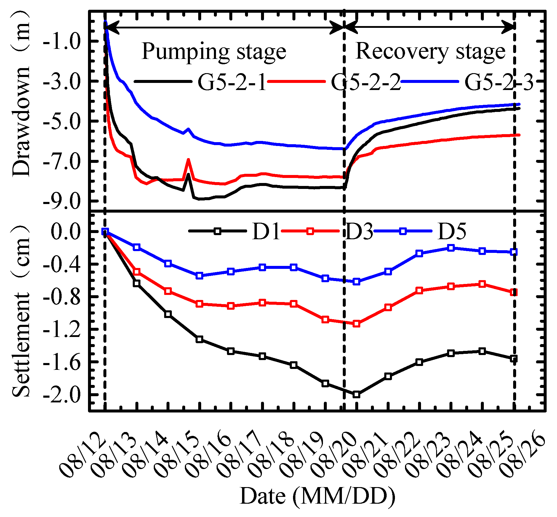
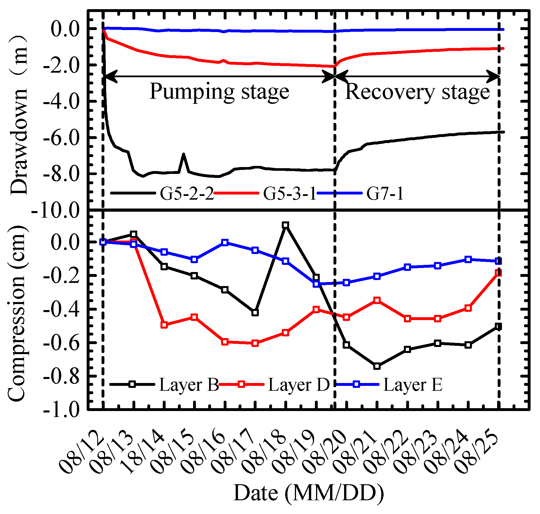
4.1. Responses of Groundwater Level

As aforementioned, the MCA concerned in this study is directly connected with Aq I. For this reason, dewatering in the MCA can also induce the groundwater drawdowns in its adjacent aquifers. To investigate the hydraulic connection between MCA and Aq I as well as its influence on groundwater fluctuations, the responses of groundwater level in different aquifers during the field tests are analyzed in this section.

4.1.1. Test Results

Figure 5 presents the discharge rates of the pumping wells and the groundwater level obtained in the observation wells. In the C5-2-1 pumping test, the groundwater head in Layers ⑤2~⑤3-2 had a rapid decline at the beginning and then decreased slowly until it reached a steady value, whereas the drawdowns observed in Layer ⑤3-3 and Layer ⑦ were relatively small. Specifically, the maximum drawdowns obtained using G5-2-1~G5-2-3 in Layers ⑤2~⑤3-2 were 1.75 m, 1.18 m and 0.74 m, respectively, while those monitored by G5-3-1 in Layer ⑤3-3 and G7-1 and G7-2 in Layer ⑦ were almost negligible, with the maximum drawdown of 0.14 m, −0.22 m, and −0.1 m, respectively, where minus meant head increment. A similar phenomenon was also observed from the C5-3-1 and the C7-1 pumping well test. The maximum drawdowns monitored by G5-2-1~G7-2 in the C5-3-1 pumping well test were 0.44 m, 0.23 m, 0.12 m, 2.04 m, 0.56 m, and 0 m, respectively, while those in the C7-1 pumping well test were 0.01 m, 0.02 m, −0.01 m, 0.03m, 1.23 m and 0.94m, respectively. In addition, once the dewatering was interrupted, the groundwater head recovered immediately.

When the multi-well pumping test was conducted in Layers ⑤2~⑤3-2 using well C5-2-1~C5-2-4, besides obvious drawdowns observed in the pumping aquifer, maximum drawdowns of 8.18 m monitored in well G5-2-1, 7.25 m in well G5-2-2, and 6.26 m in well G5-2-3, an inconspicuous but not negligible drawdown of 1.59 m monitored in well G5-3-1 was also observed in the underneath Layer ⑤3-3 as well as a 0.05-m-deep drawdown monitored in G7-1 and a 0.13-m-deep drawdown monitored in G7-2 traced in Layer ⑦. The groundwater drawdown rate in Layers ⑤2~⑤3-2 was large at the beginning and then declined gradually until it reached a steady level. The groundwater head in Layer ⑤3-3 and Layer ⑦ also followed the same development law. After the multi-well pumping test was shut down, the groundwater head in each aquifer recovered immediately. In addition, the groundwater head in Layers ⑤2~⑤3-2 increased unexpectedly after the test continued for about 65 h due to power failure.

4.1.2. Analyses

As aforementioned, in the single-well pumping test, remarkable groundwater drawdowns could be observed in the pumping aquifers, while small but not negligible drawdowns could also be detected in other aquifers especially in the adjacent aquifers, indicating that there were hydraulic connections and a leakage effect among each aquifer. The hydraulic connection and leakage effect were more easily observed in the multi-well pumping test because the accumulated discharge rate and operation time were much larger than those in the single-well pumping tests. In real field work, the dewatering is usually performed using multi-well for several months or even more than a year [7], consequently causing apparent drawdowns in the pumping aquifer as well as its adjacent aquifers due to the hydraulic connection and leakage effect. Hence, during the excavation dewatering, although the pumping wells were only installed in Layers ⑤2~⑤3-2, the groundwater drawdowns and stratum deformation in Layer ⑤3-3 and Layer ⑦ should also be considered because of the hydraulic connection and leakage effect. Otherwise, an underestimate of water inflow and land subsidence may emerge, resulting in an adverse effect on the safety of the excavation and the surroundings.

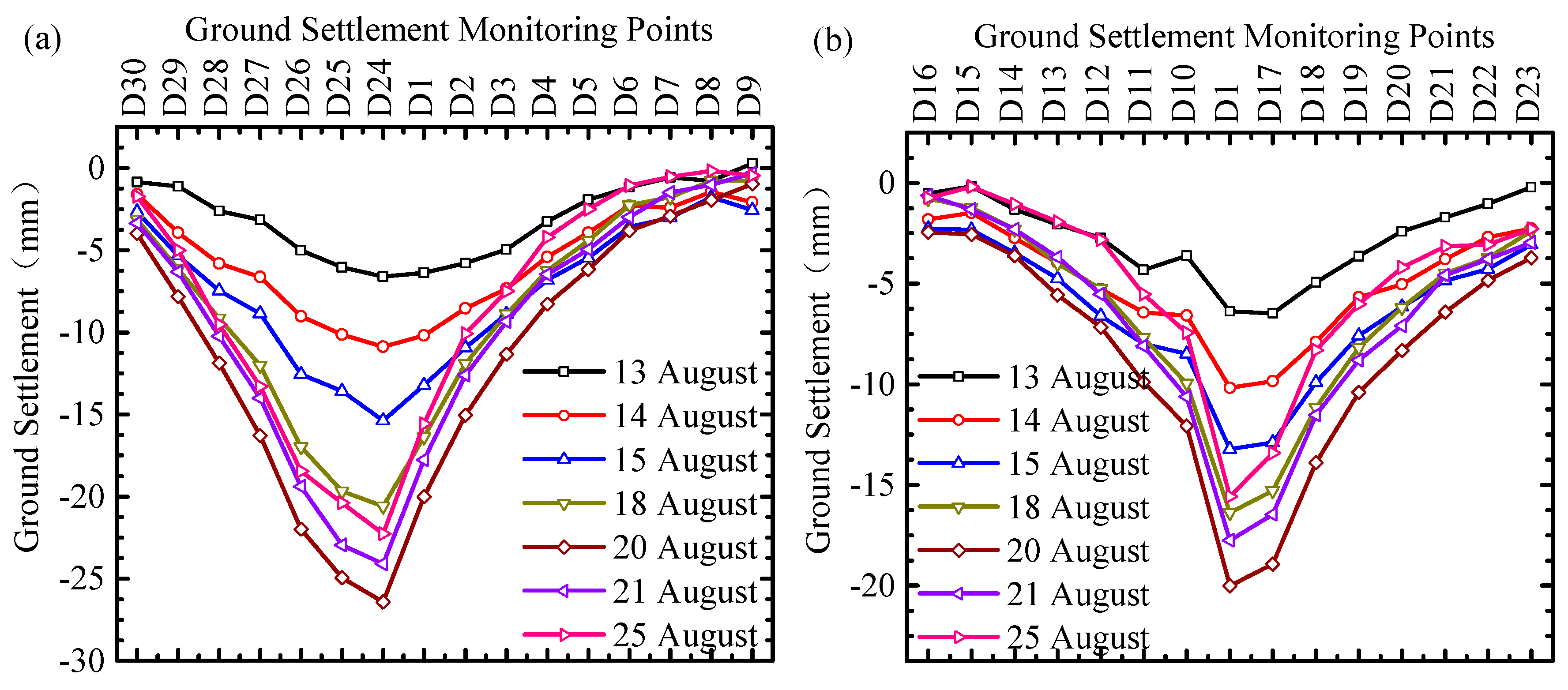
4.2. Responses of Ground Settlement

Responses of ground settlement induced by dewatering in deep confined aquifers [8,9,10,11,12] has been widely investigated, whereas few literatures focus on those due to groundwater extraction in shallow confined aquifers. In this section, the ground settlement due to dewatering in the MCA as well as the correlation between ground settlement and groundwater drawdowns is analyzed to investigate the responses of ground settlement induced by dewatering in shallow confined aquifers.

4.2.1. Results

In Figure 6, the distributions of ground settlements obtained by the 30 monitoring points (D1 to D30) during the multi-well pumping test are depicted. As can be seen in Figure 6, the ground settlement increased gradually with the proceeding of the pumping test and reached its maximum value at the end of the test (Aug. 20th). After that, a remarkable rebound of ground settlement could be observed. Besides, it is notable that the distributions of ground settlement at different stages of the test were similarly shown in bell-shaped distribution. The settlement was larger when the distance of monitoring point to the pumping center was smaller and reached its maximum value at the monitoring point D24. Additionally, the settlement at the left side of D1 was apparently larger than that at the right side, which was inconsistent with the groundwater drawdown. The possible reason responsible for this may be the soil erosion and ground collapse induced by high-speed groundwater flow.

Furthermore, the time-history curves for the settlement of D1, D3, and D5 as well as the drawdowns in G5-2-1, G5-2-2, and G5-2-3 (next to D1, D3, and D5, respectively) are observed in Figure 7. As can be seen, the development of the settlement was similar to that of the drawdown observed in the adjacent well. The rate of ground settlement varied in proportion to that of groundwater drawdowns, and a larger ultimate value of groundwater drawdown would cause a greater ultimate value of ground settlement. Once the multi-well pumping was terminated, the groundwater level recovered immediately, and the surface subsidence rebounded subsequently. As can be seen in Figure 7, slight hysteresis can be observed between the development of groundwater drawdowns and ground settlement. The possible reason responsible for this phenomenon could be that the aquitard and phreatic aquifer overlying the pumping aquifer limit the delivery and accumulation of the stratum deformation.

4.2.2. Analyses

Groundwater extraction would reduce the artesian head and pore pressure in the pumping aquifer as well as its adjacent aquifers, causing the increase of effective stress and finally resulting in the compression of pumping aquifers, which is the primary reason for ground settlement [3]. Thus, needless to say, the distributions of the ground settlement should be parallel to those of drawdowns. According to test results, the conclusion is tenable in the most areas of the test site except the immediate vicinity of pumping wells, where the ground settlement was a little larger, e.g., the settlement of D24. As aforementioned, the possible reason may be soil erosion and ground collapse. In fact, the average discharge rate of pumping well C5-2-2 was 15.64 m³/h with the maximum value of over 25 m³/h, making the groundwater flow to C5-2-2 at a higher speed. This high-speed flow, carrying along plenty of soil particles, flowed out of underground through pumping wells, consequently causing ground collapse and unexpected settlement. Moreover, the collapse-induced settlement was unrecoverable. Thus, the settlement could not rebound sufficiently as the drawdown did in the recovery stage (see Figure 7).

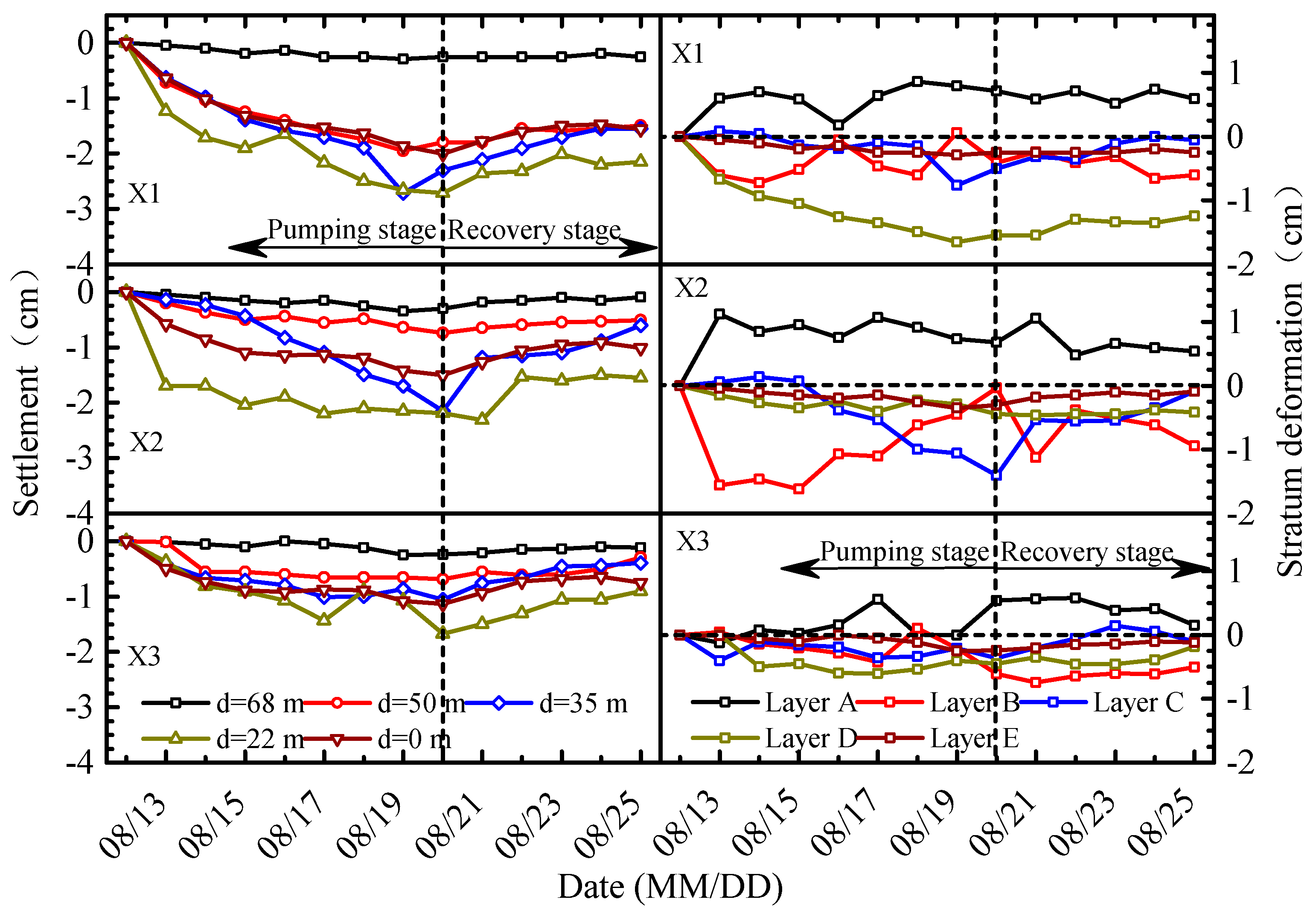
4.3. Responses of Deep Soil Deformation

Both engineering practices and theoretical researches have revealed that the dewatering-induced settlement of deep soil can be larger than that of the ground surface [8]. In this section, to investigate the responses of deep soil deformation, the soil settlement at different depths as well as its correlation to the groundwater fluctuations is analyzed.

4.3.1. Results

On the left part of Figure 8 are the history curves for deep soil settlement monitored by X1~X3. The data of X4 were absent due to technical failures. As can be seen, during the pumping stage, the soil at various depths and positions firstly subsided gradually until the pumping was shut down and shortly afterwards rebounded progressively with groundwater recovery. At the same depth, the subsidence of the monitoring point was larger as its distance to the pumping center became closer. In the same monitoring hole, the soil at a depth of 22 m suffered the largest subsidence for most of the time, followed by that at a depth of 35 m (in X1 and X2) or the surface soil (in X3), whereas that at a depth of 68 m held the smallest deformation, smaller than that at a depth of 50 m.

Subsequently, the stratum is divided into five layers by the deep soil settlement monitoring points and they are Layer A (0 m to −22 m), Layer B (−22 m to −35 m), Layer C (−35 m to −50 m), Layer D (−50 m to −68 m) and Layer E (≤−68 m), respectively, as can be seen in Figure 2. Here, Layer A refers to the soil layers overlying the MCA, Layers B, C, and D refer to the upper, middle, and lower part of the MCA, respectively, while Layer E refers to the soil layers underlying the MCA. The deformation of each layer can be obtained by subtracting the displacement at its bottom by that of its top, and positive values mean soil expansion while negative values mean soil compression. The results are depicted in the right part of Figure 8. As can be seen, there were usually four layers, including Layer B, C, D, and E, compressed to varying degrees and one layer, Layer A, expanded and the expansion decreased as the distance to the pumping center increased. Among the compressed layers, Layers B, C, and D located in the pumping aquifer (MCA) usually had relatively larger deformation while layer E in Layer ⑦ suffered the smallest compression.

Additionally, the time-history curves for the soil compression of Layers B, D, and E in X3 and the corresponding drawdowns monitored by G5-2-2, G5-3-1, and G7-1 (next to X3) are depicted in Figure 9. As demonstrated, the development of soil compression in the pumping stage was irregular, whereas that in the recovery stage showed good correlation with the development of the groundwater fluctuations in the same layer. The larger the drawdown was, the more severely the soil compressed, also indicating that dewatering-induced drawdown was an important reason for ground settlement.

4.3.2. Analyses

As aforementioned, there was expansion in Layer A, and that was why the maximum subsidence usually occurred at the top of the pumping aquifer instead of the ground surface. The reason for soil expansion could be attributed to dewatering-induced differential drawdowns and compression in the pumping aquifer. During the test, although there were no obvious drawdowns in Layer A, whereas to satisfy deformation coordination, uneven downward displacement took place at the bottom of Layer A, which induced the rotation of principal stress and the formation of stress arch in Layer A due to surrounding constraint and caused the expansion of Layer A. In addition, as observed in Figure 8 and Figure 9, the distributions and development of the stratum deformation were relatively irregular. The possible reasons, including compressibility, body force, and stress history of soil, piping erosion, and ground collapse due to high-speed flow as well as the influence of partially penetrating well, etc., are various and complex. Therefore, further study on this issue is still imminently required.

5. Back Analysis of Groundwater Fluctuations and Ground Settlement

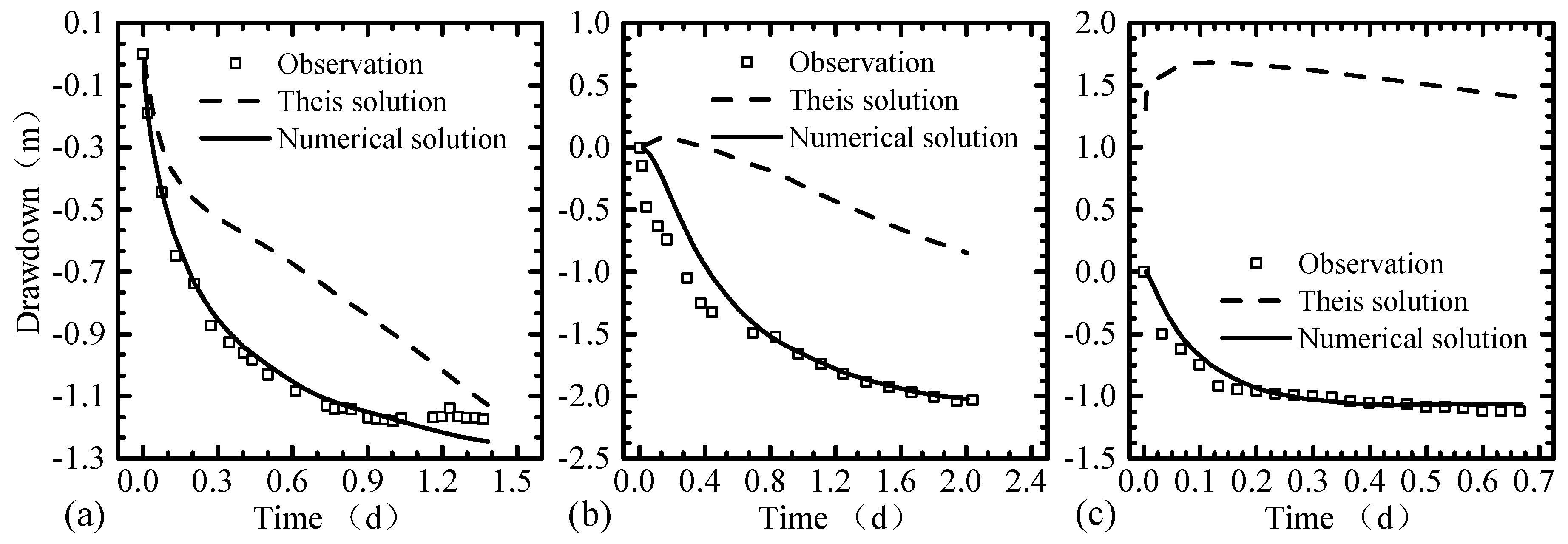
5.1. Hydrogeological Parameter Estimation Based on Pumping Well Test

5.1.1. Limitations of the Analytical Methods

For the prediction model of groundwater drawdown and stratum deformation, in addition to accurate mechanisms of groundwater seepage, the precise parameters of pumping aquifers play significant roles for the final results. Several mathematical models and corresponding analytical or semi-analytical solutions have been proposed for aquifer parameter estimation [38,39,40,41,42,43,44,45,46]. These models can consider the influence of leaky aquifers [40,41] or variable discharge [42,45] to a certain degree. However, the preceding models assume homogeneous, isotropic, and laterally-unbounded aquifers. Nevertheless, in reality, the aquifer is much more complicated than the previously-assumed aquifer aforementioned. Real aquifers are generally characterized by anisotropy and leakage effect, resulting in the above models being not accurate enough for the description of groundwater flow and estimation of aquifer parameters.

5.1.2. Parameter Estimation using Numerical Method

This research mainly focuses on an aquifer system consisting of several micro-confined and confined aquifers. Considering the complexity of the hydrogeology and the limitations of the analytical methods, the numerical method is more reliable and recognized for parameter estimation [47,48,49,50]. In this study, a three-dimensional numerical model is developed in Visual Modflow [51] for groundwater drawdown calculation. In the model, the leaky aquifers are considered by simulating the real site conditions, whereas the variable injection rate is considered by setting a pumping schedule in the software. Moreover, the parameter estimation program PEST of Visual Modflow has been adopted for hydrogeological parameter estimation [51]. The following steps are undertaken for the parameter estimation using numerical method:

Step 1: Develop a numerical model based on the site condition and calculate the groundwater drawdowns in observation wells due to single-well pumping with the parameters obtained using the Hantush–Jacob solution.

Step 2: Call PEST for the parameter optimization of Layers ⑤2~⑤3-2 and update the parameters.

Step 3: Call PEST for the parameter optimization of Layer ⑤3-3 and update the parameters.

Step 4: Recalculate the groundwater drawdowns in Layers ⑤2~⑤3-2 and compare the discrepancy between the results of Step 4 and Step 2. Repeat step2 and step 3 until the discrepancy is sufficiently small.

Step 5: Call PEST for parameter optimization for Layer ⑦ and check the influence of parameter optimization on groundwater level in other aquifers. Repeat Step 2 and Step 3 until the influence can be negligible.

5.1.3. Results and Analyses

In this section, the proposed numerical method is employed for parameter estimation as well as an analytical method based Theis solution.

Table 3. Comparison between the parameter obtained by the analytical and numerical method.

Estimation Method		Theis Method	Numerical Solution
Layers ⑤2~⑤3-2	kh (cm/s)	3.73 × 10−3	1.02 × 10−2
	kv (cm/s)	3.73 × 10−3	3.58 × 10−3
	S	4.07 × 10−4	8.90×10−4
Layer ⑤3-3	kh (cm/s)	1.68 × 10−3	4.51 × 10−4
	kv (cm/s)	1.68 × 10−3	1.50 × 10−4
	S	2.44 × 10−4	9.12 × 10−4
Layer ⑦	kh (cm/s)	4.86 × 10−2	9.21 × 10−3
	kv (cm/s)	4.86 × 10−2	3.84 × 10−3
	S (10−4)	9.80 × 10−6	1.44 × 10−3

lists the results for parameter estimation. The estimation value using the analytical method is larger in hydraulic conductivity and smaller in storage than that using the numerical method in Layer ⑤3-3 and Layer ⑦, while it is the opposite in Layers ⑤2~⑤3-2. Moreover, the drawdowns are calculated in Visual Modflow using the two group of parameters, and the results are depicted in Figure 10 as well as the observed drawdowns. As can be seen, the calculated drawdowns using the proposed numerical method match the observed drawdowns well except at the early stage of pumping when the discharge rate is unstable, whereas those using the analytical method present significant discrepancy with the observed drawdowns, indicating that the proposed numerical method is more reliable for parameter estimation and drawdown calculation in complex aquifer systems.

As mentioned earlier, there are significant discrepancies between the numerical results and the analytical ones. The primary reason for this is the hydraulic connection among each aquifer. When pumping in Layer ⑤3-3 or Layer ⑦, the head in the pumping aquifer decreased rapidly, and head difference was formed, causing the groundwater from the adjacent aquifers to flow into the pumping aquifer. When pumping in Layers ⑤2~⑤3-2, significant drawdowns could be widely observed in the pumping aquifer. However, the natural head in this layer was relatively larger than that in Layer ⑤3-3 before dewatering, and this held true for most areas during dewatering, resulting in the groundwater flowed into Layer ⑤3-3. In analytical methods, the aquifers were assumed to be entirely isolated. Thus, the groundwater flowing into or out of the pumping aquifer is oversimplified, causing the hydraulic conductivity in Layer ⑤3-3 and Layer ⑦ was overrated and that in Layers ⑤2~⑤3-2 was underestimated. Whereas, in the numerical method this characteristic could be considered by developing a unified numerical model according to the site condition. Consequently, the numerical method is more accurate for parameter identification in complex aquifer systems.

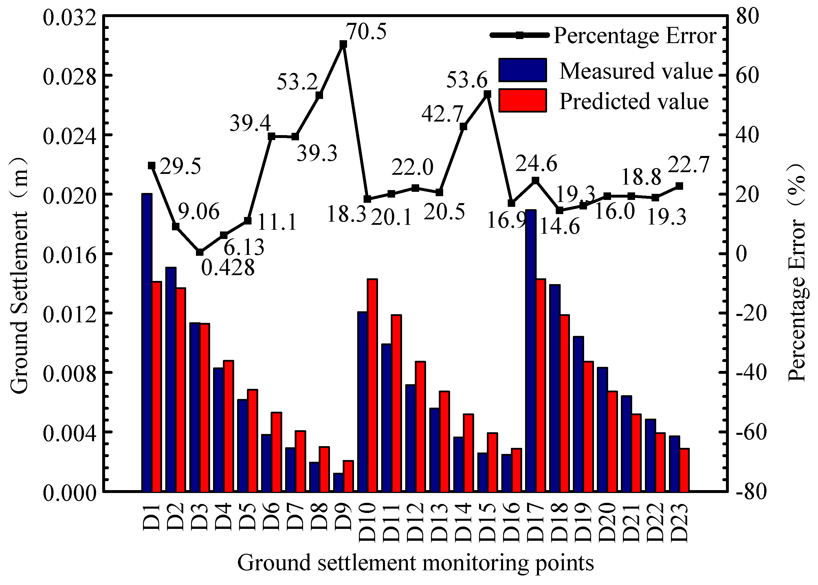
5.2. Ground Settlement Prediction Induced by Dewatering

5.2.1. Basic Assumptions

In this section, a simple prediction method for ground settlement induced by dewatering is proposed and discussed. In this method, the conventional Theis Model is employed to calculate the drawdowns due to dewatering, and the unidirectional compression formula is utilized to estimate the soil compression. Hence, the assumptions used in this method are identical to those in the Theis Model except that the compression of the pumping aquifer is assumed to be completed instantly and equal to the ground settlement. This assumption is conservative considering the expansion of the overlying non-pumping layers. Besides, the assumptions above cannot consider many factors related to the geological condition, such as the body force and stress history of soil. However, these factors can be considered indirectly by calibrating the predicting result using the observation data.

5.2.2. Ground Settlement Prediction Based on Pumping Well Test

In application, the following steps may be taken to calculate the dewatering-induced ground settlement:

Step 1: Calculate the groundwater drawdown induced by single-well pumping based on Theis Formula.

Step 2: Acquire the groundwater drawdown caused by multi-well pumping using the superposition principle.

Step 3: Obtain the additional effective stress due to groundwater drawdown by the theory of effective stress.

Step 4: Develop the prediction expression for settlement utilizing unidirectional compression formula.

Step 5: Compute the undetermined coefficients in the expression with the observation data.

According to the aforementioned, the expression for ground settlement prediction can be described as follows (details can be found in the Appendix A):

$$\Delta s=\frac{{\gamma }_{w}H}{E_s}{\displaystyle \sum _{i=1}^n\left(\frac{2.3Q_i}{4\pi T}·\lg \frac{2.25Tt}{S}-\frac{2·2.3Q_i}{4\pi T}·\lg r_i\right)}={\displaystyle \sum _{i=1}^n{J}_i·\lg t-K_i·\lg r_i+L_i}$$

(1)

where $\Delta s$ is the ground settlement [L] at distance $r$ [L] and time $t$ [T]; $E_s$ is the compressing modulus [ML⁻¹T⁻²]; $H$ is the thickness [L] of the pumping aquifer; ${\gamma }_w$ the bulk density [ML⁻²T⁻²] of water; $Q$ is the discharge rate [L³T⁻¹]; $T$ is the transmissivity [L²T⁻¹], and $S$ is the storage coefficient [dimensionless]. Besides, $J_i$, $K_i$ and $L_i$ are undetermined coefficients and can be expressed as $J_i=\frac{2.3{\gamma }_{w}H{Q}_i}{4\pi T{E}_s}$, $K_i=\frac{2·2.3{\gamma }_{w}H{Q}_i}{4\pi T{E}_s}$ and $L_i=\frac{2.3{\gamma }_{w}H{Q}_i}{4\pi T{E}_s}·\lg \left(2.25T/S\right)$. The undetermined coefficients follow the relationships: $J_1:J_2:\cdots :J_n=K_1:K_2:\cdots :K_n=L_1:L_2:\cdots :L_n=Q_1:Q_2:\cdots :Q_n$, $K_i=2J_i$, and can be determined using the nonlinear curve fitting function of the Origin software based on the ground settlement observation data.

5.2.3. Validation and Analyses

During the test, there were four pumping wells employed. Thus, the total number of the undetermined coefficient was 12. Subsequently, these undermined coefficients were determined by performing the nonlinear fitting according to Equation (1) based on the ground settlement observation data of D1~D23 from Day 4 to Day 7. The results are shown as: $J_1$ = 0.00128, $J_2$ = 0.00275, $J_3$ = 0.00205, $J_4$ = 0.00191, $K_1$ = 0.00256, $K_2$ = 0.00550, $K_3$ = 0.00410, $K_4$ = 0.00382, $L_1$ = 0.00228, $L_2$ = 0.00490, $L_3$ = 0.00366, $L_4$ = 0.00340, and the goodness of fitting is 0.870. Further, the predicting formula is employed to predict the ground settlement on Day 8, and the predictive values and observation values, as well as the error analyses, are depicted in Figure 11.

As illustrated in Figure 11, the percentage errors vary from 0.428% to 70.5% with an average value of 25.57%. The prediction method functioned well for a majority of the monitoring points with a percentage error of less than 25%. However, for the points at the far-field (such as D9 and D15) of the test site, the error was much larger and even exceeded 50%. At the far-field, the ground settlement induced by groundwater extraction was very small, usually 2~3 mm. For this reason, the error caused by human activities and measurements was inevitable and considerable. In addition, at the central part of the test site, the measured value of subsidence was usually larger than the prediction value. The possible reason may be the aforementioned ground collapse due to high-speed groundwater flow. In general, the prediction values match well with the observation data, indicating that the prediction method proposed in this paper is feasible.

6. Conclusions

In this paper, field pumping well tests were performed in Pudong New Aera to investigate the responses of the groundwater level and stratum deformation due to dewatering in the MCA. On this basis, practical methods for hydrological parameter estimation and ground settlement prediction were proposed and discussed. Following conclusions can be drawn:

(1) Both the single-well and multi-well pumping tests indicate that there is a close hydraulic connection between MCA and Aq I. Hence, even if dewatering measurements are only performed in MCA, the groundwater drawdowns and stratum deformation in Aq I should be considered to avoid underestimating water inflow and ground settlement.

(2) The distributions and development of ground settlement are similar to those of groundwater drawdowns. It is tenable for most areas except the immediate vicinity of the pumping wells, where the subsidence is larger and cannot rebound sufficiently with groundwater recovery due to ground collapse induced by high-speed groundwater flow.

(3) During the pumping well test, soil settlement and stratum compression can be observed not only in the pumping aquifer but also in its underlying aquifers and their distributions and development show correlation with those of groundwater fluctuations, which also indicates there is a close hydraulic connection among each aquifer.

(4) During the pumping well test, because a stress arch is formed in the top layer due to uneven deformation and surrounding constraint, the top layer is expanded, and the largest subsidence usually occurs at the top of the pumping aquifer instead of the ground surface.

(5) For the parameter estimation under complex hydrogeology conditions, especially when the micro-confined aquifer is directly connected with the deep confined aquifer, the proposed numerical method can consider the effect of hydraulic connection, and the results are more reliable and accurate compared with those of the conventional analytical methods.

(6) The proposed prediction method for the dewatering-induced ground settlement functions well at most parts of the test site except at the far-field and the central parts, indicating its feasibility. Moreover, the parameters used in the method can be obtained by performing fitting with observation data, avoiding the dependence on precise hydrogeological parameters.

References

1. Shanghai Geology Office (SGO). Report on Land Subsidence in Shanghai (1962–1976); SGO: Shanghai, China, 1979. (In Chinese) [Google Scholar]
2. The Institute of Hydrogeology and Engineering Geology (IHEG). Hydrogeological map of Shanghai, Hydrogeological in Atlas of China, No. 45; IHEG: Shanghai, China, 1979. (In Chinese) [Google Scholar]
3. Chai, J.C.; Shen, S.L.; Zhu, H.H.; Zhang, X.L. Land subsidence due to groundwater drawdown in Shanghai. Géotechnique 2004, 56, 143–147. [Google Scholar] [CrossRef]
4. Xu, Y.; Shen, S.; Du, Y. Geological and hydrogeological environment in Shanghai with geohazards to construction and maintenance of infrastructures. Eng. Geol. 2009, 109, 241–254. [Google Scholar] [CrossRef]
5. Xu, Y.; Shen, S.; Ma, L.; Sun, W.; Yin, Z. Evaluation of the blocking effect of retaining walls on groundwater seepage in aquifers with different insertion depths. Eng. Geol. 2014, 183, 254–264. [Google Scholar] [CrossRef]
6. Shanghai Geology and Minerals Topology Editorial Board (SGMTEB). Shanghai Geology and Minerals Topology (SGMT); Shanghai Academy of Social Science Press: Shanghai, China, 1999. (In Chinese) [Google Scholar]
7. Zeng, C.F.; Xue, X.L.; Zheng, G.; Xue, T.Y.; Mei, G.X. Responses of retaining wall and surrounding ground to pre-excavation dewatering in an alternated multi-aquifer-aquitard system. J. Hydrol. 2018, 559, 609–626. [Google Scholar] [CrossRef]
8. Zheng, G.; Zeng, C.F.; Xue, X.L. Settlement mechanism of soils induced by local pressure-relief of confined aquifer and parameter analysis. Chin. J. Geotech. Eng. 2014, 36, 802–807. (In Chinese) [Google Scholar]
9. Zhang, Y.; Li, M.; Wang, J.; Chen, J.; Zhu, Y. Field tests of pumping-recharge technology for deep confined aquifers and its application to a deep excavation. Eng. Geol. 2017, 228, 249–259. [Google Scholar] [CrossRef]
10. Zhang, Y.; Wang, J.; Chen, J.; Li, M. Numerical study on the responses of groundwater and strata to pumping and recharge in a deep confined aquifer. J. Hydrol. 2017, 548, 342–352. [Google Scholar] [CrossRef]
11. Wang, J.; Feng, B.; Liu, Y.; Wu, L.; Zhu, Y.; Zhang, X.; Tang, Y.; Yang, P. Controlling subsidence caused by de-watering in a deep foundation pit. Bull. Eng. Geol. Environ. 2012, 71, 545–555. [Google Scholar] [CrossRef]
12. Xu, Y.; Yuan, Y.; Shen, S.; Yin, Z.; Wu, H.; Ma, L. Investigation into subsidence hazards due to groundwater pumping from Aquifer II in Changzhou, China. Nat. Hazards 2015, 78, 281–296. [Google Scholar] [CrossRef]
13. Zheng, G.; Dai, X.; Diao, Y.; Zeng, C.F. Experimental and simplified model study of the development of ground settlement under hazards induced by loss of groundwater and sand. Nat. Hazards 2016, 82, 1869–1893. [Google Scholar] [CrossRef]
14. Shanghai Geotechnical Engineering Survey and Design Research Institute (SGESDRI). Code for Investigation of Geotechnical Engineering; SGESDRI: Shanghai, China, 2012. (In Chinese) [Google Scholar]
15. Zhang, H.; Liu, M. “Feeble confined water” in Shanghai area and related geotechnical engineering problems in foundation excavation. Chin. J. Geotech. Eng. 2005, 27, 944–947. (In Chinese) [Google Scholar]
16. Wei, T.Y.; Chen, Z.Y.; Wei, Z.X.; Wang, Z.Q.; Wang, Z.H.; Yin, H.F. The distribution of geochemical trace elements in the Quaternary sedments of the Changjiang River Mouth and the paleo environmental implications. Quat. Sci. 2006, 26, 397–405. (In Chinese) [Google Scholar]
17. Wei, Z.X. Quaternary Environmental Evolution in Eastern Yangtze Delta: Coupling of Neotectonic Movement, Paleoclimate and Sea-Level Fluctuation. Ph.D. Thesis, East China Normal University, Shanghai, China, 2003. (In Chinese). [Google Scholar]
18. Chen, J.; Wang, J.; Zhang, J.; Zhang, L.; Zhu, Y. Field Tests, Modification, and application of deep soil mixing method in soft clay. J. Geotech. Geoenviron. 2013, 139, 24–34. [Google Scholar] [CrossRef]
19. Li, M.; Zhang, Z.; Chen, J.; Wang, J.; Xu, A. Zoned and staged construction of an underground complex in Shanghai soft clay. Tunn. Undergr. Space Technol. 2017, 67, 187–200. [Google Scholar] [CrossRef]
20. Shen, S.; Wu, H.; Cui, Y.; Yin, Z. Long-term settlement behaviour of metro tunnels in the soft deposits of Shanghai. Tunn. Undergr. Space Technol. 2014, 40, 309–323. [Google Scholar] [CrossRef]
21. Liao, C.; Chen, J.; Zhang, Y. Accumulation of pore water pressure in a homogeneous sandy seabed around a rocking mono-pile subjected to wave loads. Ocean Eng. 2019. [Google Scholar] [CrossRef]
22. Chen, J.; Zhu, Y.; Li, M.; Wen, S. Novel excavation and construction method of an underground highway tunnel above operating metro tunnels. J. Aerosp. Eng. 2015, 28, A4014003. [Google Scholar] [CrossRef]
23. Li, M.G.; Wang, J.H.; Chen, J.J.; Zhang, Z.J. Responses of a Newly Built Metro Line Connected to Deep Excavations in Soft Clay. J. Perform. Constr. Facil. 2017, 31, 04017096. [Google Scholar] [CrossRef]
24. Wei, B.; Tan, Y. Performance of an Overexcavated Metro Station and Facilities Nearby. J. Perform. Constr. Facil. 2012, 26, 241–254. [Google Scholar]
25. Wu, Y.; Shen, S.; Xu, Y.; Yin, Z. Characteristics of groundwater seepage with cut-off wall in gravel aquifer. I: Field observations. Can. Geotech. J. 2015, 52, 1526–1538. [Google Scholar] [CrossRef]
26. Zheng, G.; Cao, J.; Cheng, X.; Ha, D.; Wang, F. Experimental study on the artificial recharge of semiconfined aquifers involved in deep excavation engineering. J. Hydrol. 2018, 557, 868–877. [Google Scholar] [CrossRef]
27. Wang, J.; Deng, Y.; Ma, R.; Liu, X.; Guo, Q.; Liu, S.; Shao, Y.; Wu, L.; Zhou, J.; Yang, T.; et al. Model test on partial expansion in stratified subsidence during foundation pit dewatering. J. Hydrol. 2018, 557, 489–508. [Google Scholar] [CrossRef]
28. Zeng, C.-F.; Zheng, G.; Xue, X.-L.; Mei, G.-X. Combined recharge: A method to prevent ground settlement induced by redevelopment of recharge wells. J. Hydrol. 2019, 568, 1–11. [Google Scholar] [CrossRef]
29. Wu, Y.X.; Shen, S.L.; Yuan, D.J. Characteristics of dewatering induced drawdown curve under blocking effect of retaining wall in aquifer. J. Hydrol. 2016, 539, 554–566. [Google Scholar] [CrossRef]
30. Pujades, E.; Vàzquez-Suñé, E.; Carrera, J.; Jurado, A. Dewatering of a deep excavation undertaken in a layered soil. Eng. Geol. 2014, 178, 15–27. [Google Scholar] [CrossRef]
31. Wang, J.; Wu, Y.; Liu, X.; Yang, T.; Wang, H.; Zhu, Y. Areal subsidence under pumping well–curtain interaction in subway foundation pit dewatering: Conceptual model and numerical simulations. Environ. Earth Sci. 2016, 75, 198. [Google Scholar] [CrossRef]
32. Zhang, X.; Yang, J.; Zhang, Y.; Gao, Y. Cause investigation of damages in existing building adjacent to foundation pit in construction. Eng. Fail. Anal. 2018, 83, 117–124. [Google Scholar] [CrossRef]
33. Chen, X.Y.; Zhang, L.L.; Chen, L.H.; Li, X.; Liu, D.S. Slope stability analysis based on the Coupled Eulerian-Lagrangian finite element method. Bull. Eng. Geol. Environ. 2019. [Google Scholar] [CrossRef]
34. Zheng, G.; Zeng, C.F.; Diao, Y.; Xue, X.L. Test and numerical research on wall deflections induced by pre-excavation dewatering. Comput. Geotech. 2014, 62, 244–256. [Google Scholar] [CrossRef]
35. Shen, S.; Xu, Y. Numerical evaluation of land subsidence induced by groundwater pumping in Shanghai. Can. Geotech. J. 2011, 48, 1378–1392. [Google Scholar] [CrossRef]
36. Li, M.G.; Chen, J.J.; Wang, J.H.; Zhu, Y.F. Comparative study of construction methods for deep excavations above shield tunnels. Tunn. Undergr. Space Technol. 2018, 71, 329–339. [Google Scholar] [CrossRef]
37. Li, M.G.; Xiao, X.; Wang, J.H.; Chen, J.J. Numerical study on responses of an existing metro line to staged deep excavations. Tunn. Undergr. Space Technol. 2019, 85, 268–281. [Google Scholar] [CrossRef]
38. Theis, C.V. The relation between the lowering of the Piezometric surface and the rate and duration of discharge of a well using ground-water storage. Eos Trans. Am. Geophys. Union 1935, 16, 519–524. [Google Scholar] [CrossRef]
39. Cooper, H.H.; Jacob, C.E. A generalized graphical method for evaluating formation constants and summarizing well-field history. Eos Trans. Am. Geophys. Union 1946, 27, 526–534. [Google Scholar] [CrossRef]
40. Hantush, M.S. Nonsteady flow to flowing wells in leaky aquifers. J. Geophys. Res. 1959, 64, 1043–1052. [Google Scholar] [CrossRef]
41. Hantush, M.S. Modification of the theory of leaky aquifers. J. Geophys. Res. 1960, 65, 3713–3725. [Google Scholar] [CrossRef]
42. Hantush, M.S. Drawdown around Wells of variable discharge. J. Geophys. Res. 1964, 69, 4221–4235. [Google Scholar] [CrossRef]
43. Papadopulos, I.S.; Cooper, H.H. Drawdown in a well of large diameter. Water Resour. Res. 1967, 3, 241–244. [Google Scholar] [CrossRef]
44. Agarwal, R.G.; Al-Hussainy, R. An Investigation of Wellbore Storage and Skin Effect in Unsteady Liquid Flow: I. Analytical Treatment. Soc. Petroleum Eng. J. 1970, 10, 279–290. [Google Scholar] [CrossRef]
45. Wen, Z.; Zhan, H.; Wang, Q.; Liang, X.; Ma, T.; Chen, C. Well hydraulics in pumping tests with exponentially decayed rates of abstraction in confined aquifers. J. Hydrol. 2017, 548, 40–45. [Google Scholar] [CrossRef]
46. Wu, Y.X.; Shen, J.S.; Cheng, W.C.; Hino, T. Semi-analytical solution to pumping test data with barrier, wellbore storage, and partial penetration effects. Eng. Geol. 2017, 226, 44–51. [Google Scholar] [CrossRef]
47. Shen, S.; Wu, Y.; Xu, Y.; Hino, T.; Wu, H. Evaluation of hydraulic parameters from pumping tests in multi-aquifers with vertical leakage in Tianjin. Comput. Geotech. 2015, 68, 196–207. [Google Scholar] [CrossRef]
48. Chen, C.; Jiao, J.J. Numerical simulation of pumping tests in multilayer wells with non-Darcian flow in the wellbore. Groundwater 1999, 37, 465–474. [Google Scholar] [CrossRef]
49. Doulgeris, C.; Zissis, T. 3D variable density flow simulation to evaluate pumping schemes in coastal aquifers. Water Resour. Manag. 2014, 28, 4943–4956. [Google Scholar] [CrossRef]
50. Calvache, M.L.; Sánchez-Úbeda, J.P.; Duque, C.; López-Chicano, M.; De la Torre, B. Evaluation of analytical methods to study aquifer properties with pumping tests in coastal aquifers with numerical modelling (Motril-Salobreña aquifer). Water Resour. Manag. 2006, 30, 559–575. [Google Scholar] [CrossRef]
51. HydroGeoLogic, Inc. MOD-HMS/MODFLOW-SURFACT ver. 4.0 User’s manual. A Comprehensive MODFLOW-Based Hydrologic Modeling System; HydroGeoLogic, Inc.: Herndon, VA, USA, 2008. [Google Scholar]
Figure 1. Typical distribution and hydro-geological profile of multi-aquifer-aquitard system (MAAS) in Shanghai central city: (a) location of Shanghai; (b) plan view for the location of Shanghai Administration Region; (c) type distribution of MAAS in Shanghai central city; (d1) schematic diagram for MAAS of Type I and Type II; (d2) schematic diagram for MAAS of Type III; (d3) schematic diagram for MAAS of Type IV; (d4) schematic diagram for MAAS of Type V.
Jmse 07 00058 g001
Figure 2. Profile of geological and hydrogeological section and well structure.
Jmse 07 00058 g002
Figure 3. Soil profile and properties at the construction site.
Jmse 07 00058 g003
Figure 4. Layout of test wells and ground settlement monitoring points: (a) Layout of test wells; (b) Layout of ground settlement monitoring points; (c) profile of ground settlement monitoring points.
Jmse 07 00058 g004
Figure 5. The time-history curves for discharge rate and groundwater level: (a) curves for discharge rate of pumping well; (b) curves for groundwater level in Layer ⑤2~⑤3-2; (c) curves for groundwater level in Layer ⑤3-3; (d) curves for groundwater level in Layer ⑦.
Jmse 07 00058 g005
Figure 6. The distributions of ground settlement: (a) curves for ground settlement of D1–D9 and D24–D30; (b) curves for ground settlement of D1, D10–D16, and D17–D23.
Jmse 07 00058 g006
Figure 7. The time-history curve of ground settlement and groundwater drawdowns.
Jmse 07 00058 g007
Figure 8. The time-history curves of deep soil settlement and stratum deformation.
Jmse 07 00058 g008
Figure 9. The time-history curves of deep soil compression and groundwater drawdowns.
Jmse 07 00058 g009
Figure 10. Comparison between observed and calculated drawdowns: (a) drawdowns in observation well G5-2-2; (b) drawdowns in observation well G5-3-1; (c) drawdowns in observation well G7-1;
Jmse 07 00058 g010
Figure 11. Comparison of the observation value and prediction value.
Jmse 07 00058 g011