Statistical Analysis of the Stability of Rock Slopes

Abstract

Physical model tests were performed in a wave flume at Deltares with rock armoured slopes. A shallow foreshore was present. At deep water, the same wave conditions were used, but by applying different water levels, the wave loading on the rock armoured slopes increased considerably with increasing water levels. This allowed an assessment of the effects of sea level rise. Damage was measured by using digital stereo photography (DSP), which provides information on each individual stone that is displaced. Two test series were performed five times. This allowed for a statistical analysis of the damage to rock armoured slopes, which is uncommon due to the absence of statistical information based on a systematic repetition of test series. The statistical analysis demonstrates the need for taking the mean damage into account in the design of rock armoured slopes. This is important in addition to characterising the damage itself by erosion areas and erosion depths. The relation between damage parameters, such as the erosion area and erosion depth, was obtained from the tests. Besides tests with a straight slope, tests with a berm in the seaward slopes were also performed. A new method to take the so-called length effect into account is proposed to extrapolate results from physical model tests to real structures. This length effect is important, but is normally overlooked in the design of rubble mound structures. Standard deviations based on the presented model tests were used.

1. Introduction

Due to sea level rise, the wave loading on sea defences can become more severe. This is especially the case for sea defences in shallow water. Depth-limited waves at the base of structures become larger when water levels increase under equal wave conditions in deep water. Thus, not only is there a direct influence of increasing water levels, which cause sea defences to become more vulnerable to wave overtopping, but wave loading is also affected by rising sea levels. Increased wave loading on structures affects wave overtopping and also the stability of the armour. Here, the effects of increasing water levels on the stability of rock armoured slopes have been studied under conditions that are equal in deep water, but more severe at the base of the structure.

Early stability formulae for armour layers were derived by [1] and [2]. For most significant port structures in deep water, concrete armour units are used in the armour layer for which the stability formula based on [2] is the state-of-the-art stability formula. The stability of rock armour layers in deep water is less relevant for practical applications since rock armour layers are often applied in shallower water. Shallow water or very shallow water can be defined as conditions where, during design, the offshore wave height reduces to 90% or less at the base of the structure. For such structures with rock armoured slopes, stability formulae based on [3] can be applied, as also recommended in [4]. In [5], it was shown that for shallow water, the spectral significant wave height (H_s = H_m0) is a better parameter to describe the influence of the wave height than the significant wave height from the time domain (H_s = H_1/3). In the present study, rock armour layers are also applied in shallow water, and both measures to characterize the significant wave height are presented in the present research. The stability of rock armoured slopes was studied by performing physical model tests in a wave flume. Tests with rock armoured slopes were performed with straight slopes and with a berm in the seaward slope. Damage was measured using digital stereo photography (DSP) and characterised by using various damage parameters. The tests on the straight slopes were performed five times, which allows for a statistical analysis of the results by taking into account the spreading in the test results (using the mean values, μ, the standard deviations, σ, and the variations, σ/μ). Besides the spreading of the test results in the wave flume (see also [6]), in reality, spreading of the damage also occurs. For longer structures, the risk that, at a particular location along this structure, the damage exceeds a specified maximum allowable damage increases. In the present paper, guidance for how to take this length effect into account in the design of rock armoured slopes is provided. The importance of the length effect is illustrated in an example based on the proposed method and the statistical information that was obtained from the physical model tests by repeating test series with the same conditions.

2. Physical Model Tests

Physical model tests were performed in the Scheldt Flume of Deltares, Delft (width 1 m, height 1.2 m, length 110 m of which 55 m was used in this study). The wave board is equipped with active reflection compensation (ARC). This means that the motion of the wave board compensates for the waves reflected by the structure, preventing them from re-reflecting back into the model. The wave board is equipped with second order wave steering. This means that second order effects of the first higher and lower harmonics are considered in the wave board motion. This wave generation system ensures that the generated waves resemble waves that occur in nature.

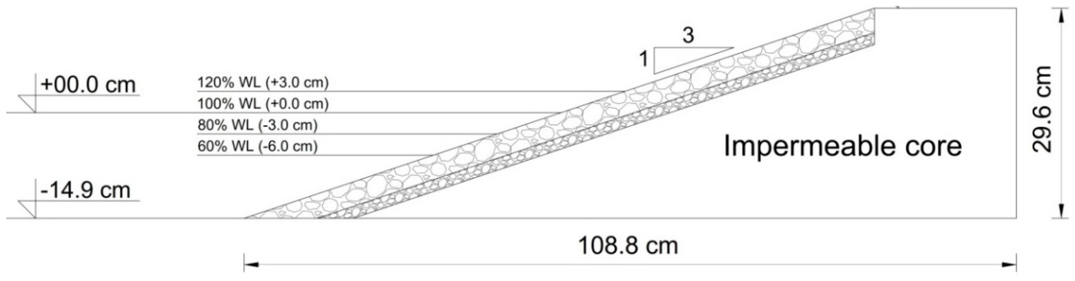
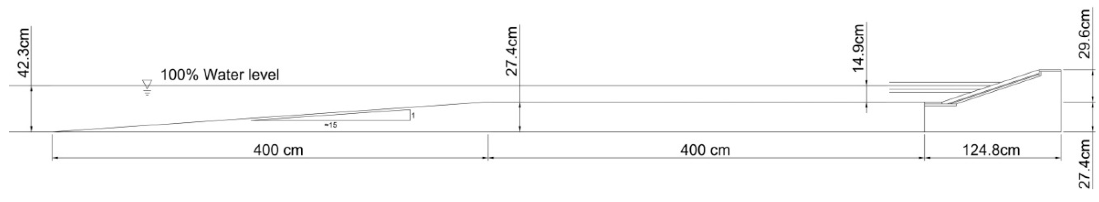
Figure 1 shows the cross-section of the test set-up in the flume. A horizontal shallow foreshore was present in front of the structure. The length of the horizontal foreshore (4 m) is long enough to ensure that the depth-limited waves that reach the structure are adapted to the (shallow) water at the base. Therefore, the foreshore is representative of other shallow foreshores, where the incident wave conditions at the base (as applied in most existing design guidelines for rock slopes) are adapted to the local water depth. The transition slope from deep water to this shallow horizontal foreshore was close to 1:15. Five structure configurations were tested. 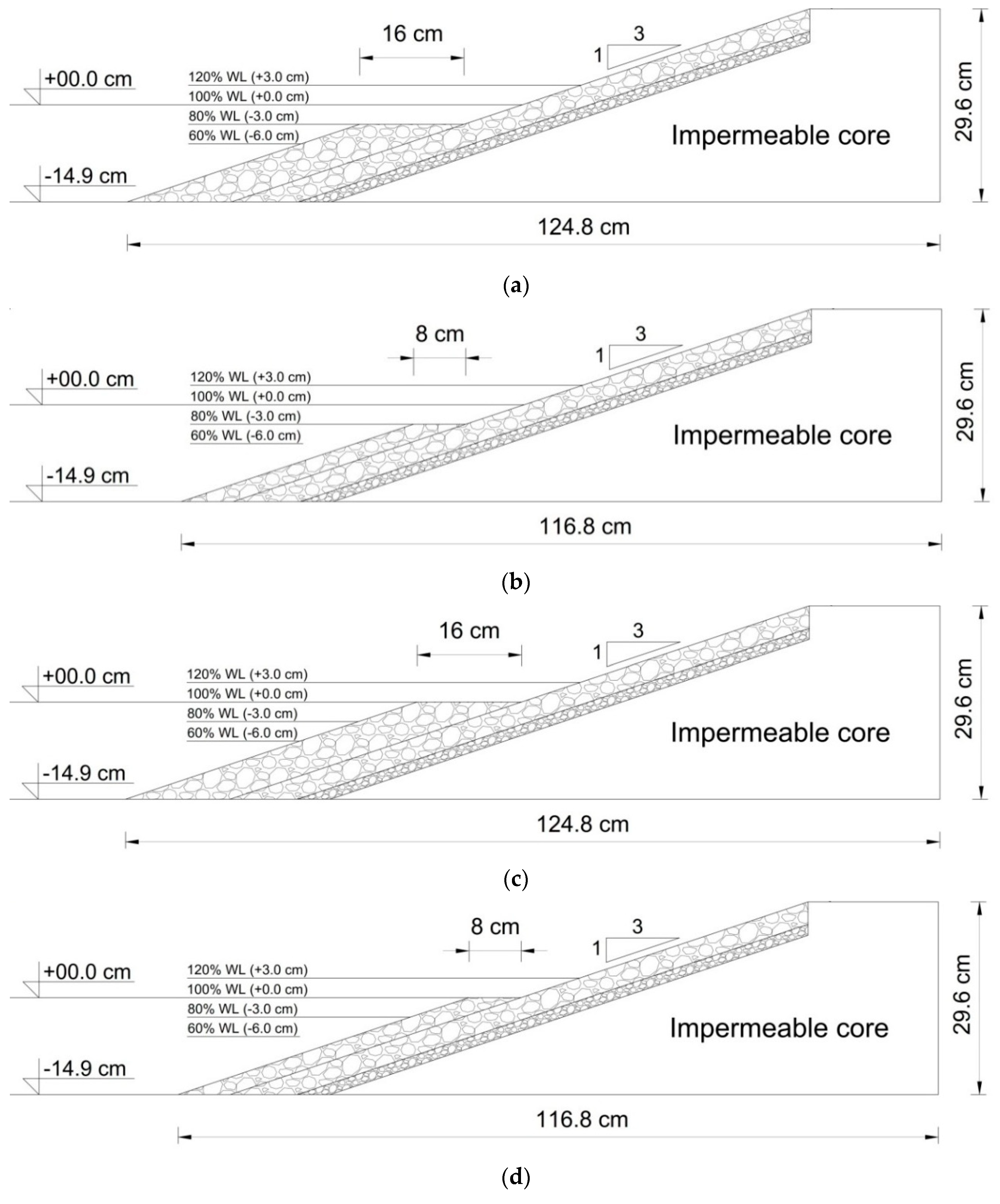One with a straight slope (see Figure 2) and four with a berm (see Figure 3): A narrow (0.08 m, i.e., a width of 5 stone diameters: 5 D_n50) and a wide berm (0.16 m, i.e., 10 D_n50), each at two different levels. The tested structures consisted of an armour layer of rock with a D_n50 of 0.0163 m, a grading of D_n85 /D_n15 = 1.25, density of ρ_s = 2710 kg/m³ and a layer thickness of two diameters, a filter layer of rock with D_n50 of 0.0094 m, and a layer thickness of two diameters, on a 1:3 slope with an impermeable core. The crest level was fixed at 0.296 m above the base of the structure (non-overtopped). The statistical analysis in the present research focuses on the structure configuration with a straight 1:3 rock slope. The tests investigated the range of damage levels that is also relevant for other structure configurations with rock armour layers (i.e., S < 12). The actual damage levels depend, for instance, on the slope and permeability of the structure, but the variation in the damage levels is assumed not to depend on the slope and permeability of the structure; the statistics of the 1:3 slope are considered representative for rock slopes with damage levels of S < 12.

The waves were measured in deep water and in front of the base of the structure. At each location, the incident waves were obtained from an array of three wave gauges. The incident deep water conditions were always the same, namely a spectral significant wave height of H_m0 = 0.088 m and a peak wave period of T_p = 1.27 s (wave steepness s_op = 0.035). Standard JONSWAP spectra were used. The number of waves was N = 1000. Each structure was tested with four different water levels (WL), resulting in water depths at still water at the base of the structure of d = 0.089 m, 0.119 m, 0.149 m, and 0.179 m (i.e., 0.03 m increase in each case).

Table 1. Measured wave conditions at deep water and at the base.

Water Level		Deep		Toe
Notation	D (m)	Hm0 (m)	Tp (s)	Hm0 (m)	H1/3 (s)	H2% (s)	Tm (s)	Tm-1,0 (s)
60%	0.089	0.088	1.27	0.039	0.030	0.035	1.21	1.59
80%	0.119	0.089	1.27	0.052	0.041	0.048	1.25	1.51
100%	0.149	0.089	1.27	0.065	0.052	0.061	1.23	1.41
120%	0.179	0.088	1.27	0.073	0.061	0.074	1.23	1.38

shows the mean values of the measured wave conditions in deep water and at the base (H_1/3 denotes the significant wave height from the time-domain analysis and T_m-1,0 is the spectral wave period characterising the effects of the wave energy spectra on the armour stability, wave run-up, wave overtopping, etc.).

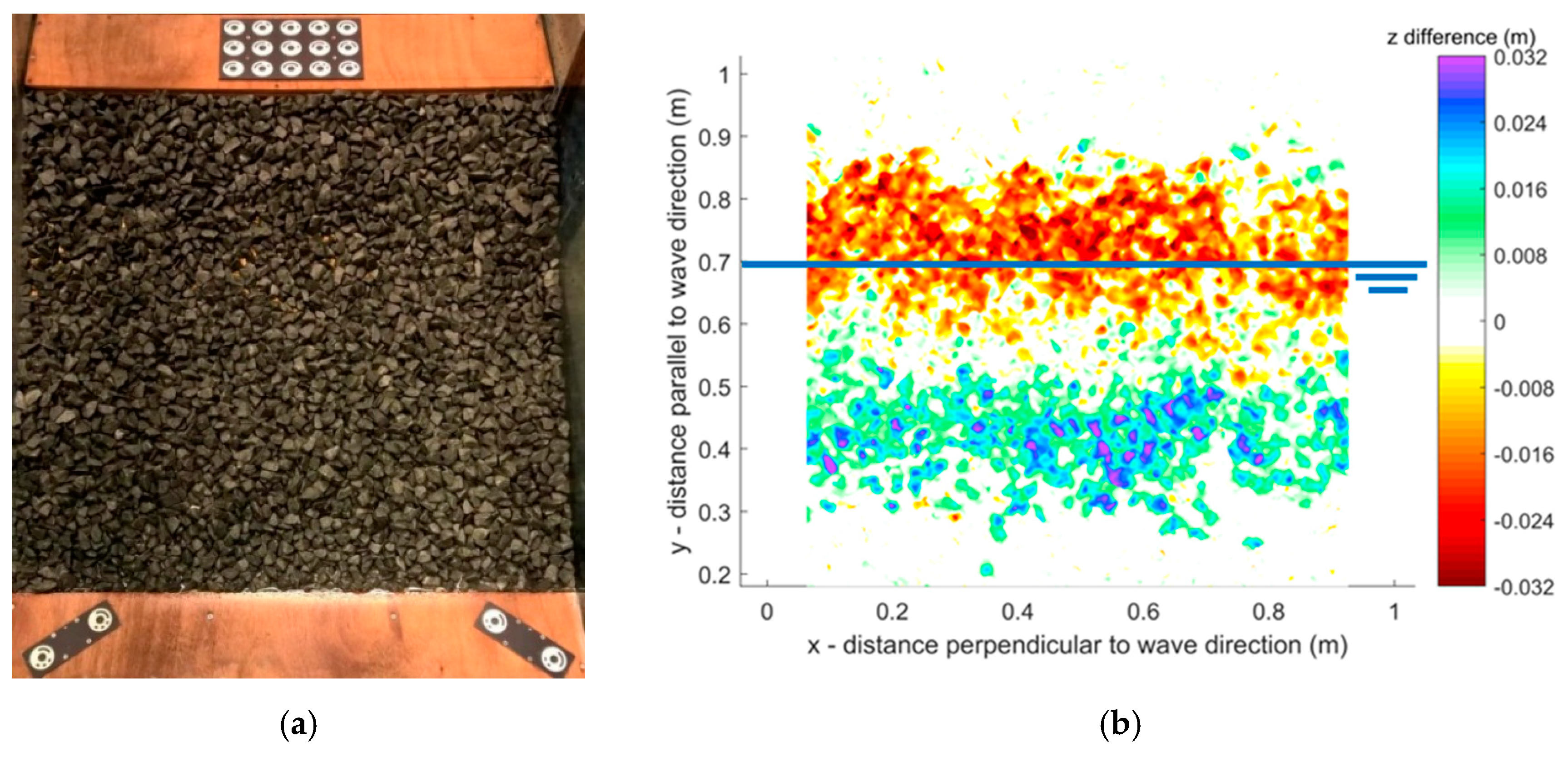
Six test series were performed, Series S1 and S2 with the structure in Figure 2, and Series S3 to S6 with one of the berm configurations in Figure 3. Except for Series S2, all series consisted of four increasing water level conditions (see Table 1) without any repair of the slope after each test, thus the resulting damage values are cumulative damage values. Series S1 with a uniform slope was performed five times. In Series S2 only the 100% condition was tested, which enabled a comparison of the results with (Series S1) and without (Series S2) milder conditions prior to the design condition. This test was also performed five times. Damage to the rock armoured slope was measured using the digital stereo photography technique (DSP) as described in [7,8]. With this measurement technique, all displaced stones can be identified by comparing the images (i.e., a 3D digital representation of the slope) after a test run with the images of the initial slope, see Figure 4. Based on this technique, all required parameters characterising the damage can be determined.

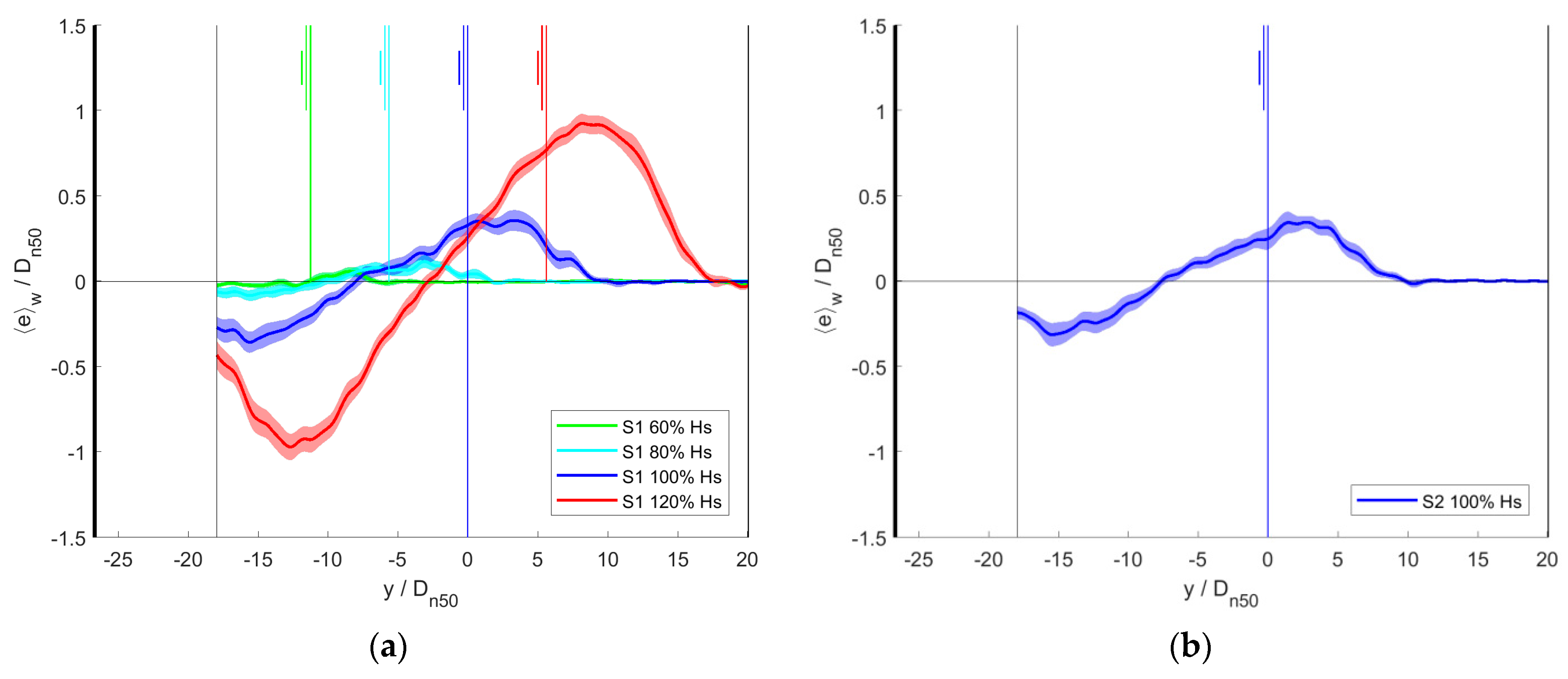
Figure 5 shows the non-dimensional erosion and deposition profiles for Series S1 and S2, averaged over five tests, including the 90% confidence intervals. On the horizontal axis, y/D_n50 denotes the intersection of the original profile of the armour and the still water level for the 100% condition. For all conditions, erosion occurs around the still water level, with the maximum erosion depth slightly above the still water level.

The following parameters were used to characterise the damage to the rock armoured slopes:

S =	Ae/Dn502 where Ae is the eroded area comparing the profiles before the tests and after a test [9] in the tests based on the average profile over the test section.
E2D =	de/Dn50 where de is the maximum depth of erosion perpendicular to the slope [6] in the tests based on the average profile over the test section.
E3D,m =	de/Dn50 where de is the maximum depth of erosion perpendicular to the slope, based on a moving average over a circular area of m Dn50 [7,8].

Here, for the parameters, S and E_2D, the values averaged over a width of 0.88 m (i.e., 54 stones with D_n50 of 0.0163 m) were used. For the parameter, E_3D,m, two values for m were used, m = 1 and m = 5.

Table 2. Test results (μ denotes the mean value of the five tests and σ denotes the corresponding standard deviation; ‘lower’ denotes the part of the slope below the berm plus the berm, and ‘upper’ denotes the slope above the berm).

Series	Condition	Slope	S		E2D		E3D,1		E3D,5
			μ	σ	μ	σ	μ	σ	μ	σ
S1	60%	Uniform 1:3	0.3	0.044	0.07	0.027	1.07	0.050	0.17	0.016
	80%		0.9	0.278	0.16	0.024	1.15	0.096	0.35	0.044
	100%		3.7	0.413	0.41	0.044	1.45	0.077	0.73	0.093
	120%		11.4	0.445	0.96	0.086	2.13	0.220	1.31	0.120
S2	100%	Uniform 1:3	3.4	0.888	0.39	0.064	1.51	0.148	0.74	0.060
			S		E2D		E3D,1		E3D,5
			lower	upper	lower	upper	lower	upper	lower	upper
S3	60%	Wide berm B = 0.16 m, hb = 0.03 m	0.1	0.0	0.03	0.00	1.13	0.12	0.18	0.01
	80%		1.1	0.0	0.15	0.01	1.11	0.25	0.28	0.02
	100%		1.7	0.3	0.25	0.08	1.35	1.15	0.44	0.20
	120%		1.5	1.0	0.25	0.16	1.35	1.15	0.38	0.38
S4	60%	Narrow berm B = 0.08 m, hb = 0.03 m	0.4	0.0	0.07	0.01	0.93	0.15	0.15	0.03
	80%		0.8	0.0	0.13	0.01	1.07	0.72	0.32	0.08
	100%		2.8	0.1	0.51	0.03	1.40	0.95	0.81	0.18
	120%		2.9	1.9	0.58	0.31	1.40	1.32	0.86	0.53
S5	60%	Wide berm B = 0.16 m, hb = 0 m	0.6	0.1	0.11	0.01	1.09	0.23	0.22	0.04
	80%		0.6	0.1	0.14	0.03	1.09	0.91	0.28	0.11
	100%		0.6	0.3	0.16	0.05	1.24	1.07	0.24	0.18
	120%		1.2	3.4	0.19	0.45	1.27	1.30	0.31	0.74
S6	60%	Narrow berm B = 0.08 m, hb = 0 m	0.2	0.1	0.04	0.01	0.97	0.25	0.17	0.03
	80%		0.7	0.3	0.14	0.12	1.10	1.11	0.28	0.20
	100%		1.2	2.0	0.23	0.31	1.15	1.35	0.37	0.68
	120%		0.1	4.6	0.04	0.53	1.11	1.51	0.24	0.74

shows the test results based on the width of the measurement section (i.e., 54 stones). Since the tests in Series S1 and Series S2 were performed five times, the mean values (μ) and the standard deviations are presented (σ). The tests with berm configurations (Series S3 to S6) were not repeated (thus the numbers denote the actual test results; h_b denotes the water depth above the berm for the 100% water level condition); the damage values are provided for the lower part of the slope, including the berm (i.e., from the base of the structure to start of the upper slope), and for the upper slope. The S-values for the entire slope are the summation of the two values. For the other damage parameters, the values for the entire slope are the maximum values of the two values (since maximum damage occurs either at the lower slope or at the upper slope).

3. Analysis of Results

The following observations can be made based on the tests results summarized in Table 2:

• Increasing water levels increase the wave loading and consequently the damage to the rock armour slopes. This increase in damage depends on the parameter that is used to characterise the damage. In the present tests, the damage increased by a factor of 44 for S, 15 for E_2D, 2 for E_3D,1, and 8 for E_3D,5.
• Comparing the damage values after the 100% condition in Series S1 (with the two preceding conditions) with the 100% condition in Series S2 (without the preceding conditions) indicates that the influence of the preceding conditions on the damage values (μ) is not statistically significant. The spreading (σ) in the damage is clearly larger for the one without preceding conditions, except for the last damage parameter (E_3D,5).
• The variations (σ/μ) in the test results for the damage parameters, S and E_2D, are relatively large for low damage values. For low damage values (60% and 80% conditions), the variations for these damage parameters, S and E_2D, are, on average, comparable, but are larger than for the damage parameters, E_3D,1 and E_3D,5. Within the range of damage that is normally considered relevant, 2 < S < 12 (where S = 2 is characterised as the start of the damage and S = 12 as the failure for the tested 1:3 slope), the variations in the damage values are comparable for the various damage parameters (S, E_2D, E_3D,1, and E_3D,5). However, for the tests without milder conditions prior to the design condition (i.e., 100% water level in Series S2), the variations in the damage parameters, E_3D,1 and E_3D,5, are clearly less than for the damage parameters, S and E_2D. As will be discussed in the following analysis, these observations are affected by the width of the test section over which the damage is determined (the above observations are valid for a width of 54 stones).
• For damage values larger than S = 1, adding a berm leads to lower damage values than in the tests with a straight slope. For wider berms, the effect of the berm increases (i.e., less damage). The structures with a submerged berm (h_b = 0.03 m) show less damage to the upper slope and more damage to the lower slope than the structures with the water level at the berm (h_b = 0 m). This is similar to results shown in [10].
• If damage is characterised by E_2D or E_3D,5, the berm does not always reduce the damage values, which is also the case for higher amounts of damage (e.g., the 100% condition). The wide berms with a width of 10 stone diameters reduce the damage most effectively, irrespective of the damage parameter that is used.

As also discussed in [11], berms can be added to existing straight slopes to reduce overtopping and damage from increasing wave loading or water levels without increasing the crest level. Since the level of berms can be increased relatively easily once sea water levels increase, adding and/or modifying a berm can be a useful measure for climate adaptation.

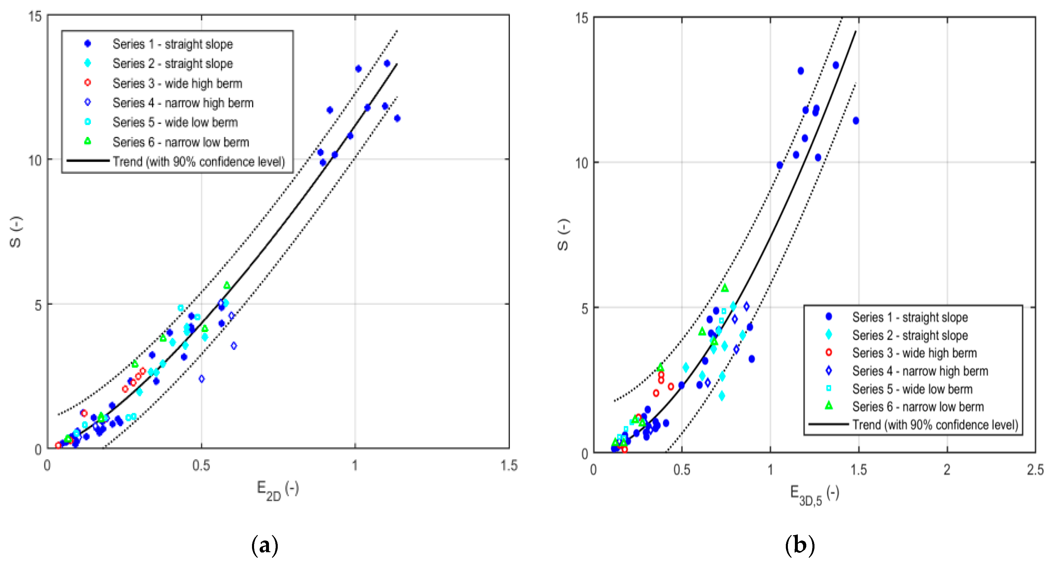
Figure 6a shows the measured damage values, S (based on the eroded area), versus E_2D (based on the erosion depth). This figure shows a clear trend between these two parameters. The relevant range of damage is often between the start of the damage (S = 2) and failure (S = 12); within this range, the trend can be simplified to S = 10 E_2D for the tested configurations (1:3 slopes, with and without a berm). Figure 6b shows the measured damage values, S (based on the eroded area), versus E_3D,5. This figure also shows a clear trend between these two parameters. Within the relevant range of damage, this trend can be simplified to S = 8 (E_3D,5)² for the tested configurations (1:3 slopes, with and without a berm).

The test results match reasonably well with existing empirical expressions for rock slope stability, with or without a berm. In [12], these comparisons were shown: For the straight slopes, the measured data is within the 90%-error bands of predictions using the stability formulae for plunging and surging waves by [3]. For the configurations with berms, the measured damage is on average somewhat lower for the part below the berm and somewhat higher for the part above the berm than predicted with the stability formulae by [10].

In the present tests, the damage was determined over a width that is equivalent to 54 stones of 0.0163 m (i.e., somewhat less than the width of the flume due to the use of markers close to the glass walls of the flume for the digital stereo photography technique). Series S1 was performed five times. Therefore, the mean damage values, the standard deviations, and the variations (i.e., the standard deviation, σ, divided by the mean values, μ) could be determined over the width of 54 stones. The statistical analysis can also be performed over a smaller width of the test section, for instance, over 10 × 27 stones instead of 5 × 54 stones (S (54) means that the mean and standard deviations of the damage are determined over a width of 54 stones, and S (27) means that the mean and standard deviations of the damage are determined over a width of 27 stones, etc.). The influence of the width of the test section (characterisation width) on the statistical values was analysed. 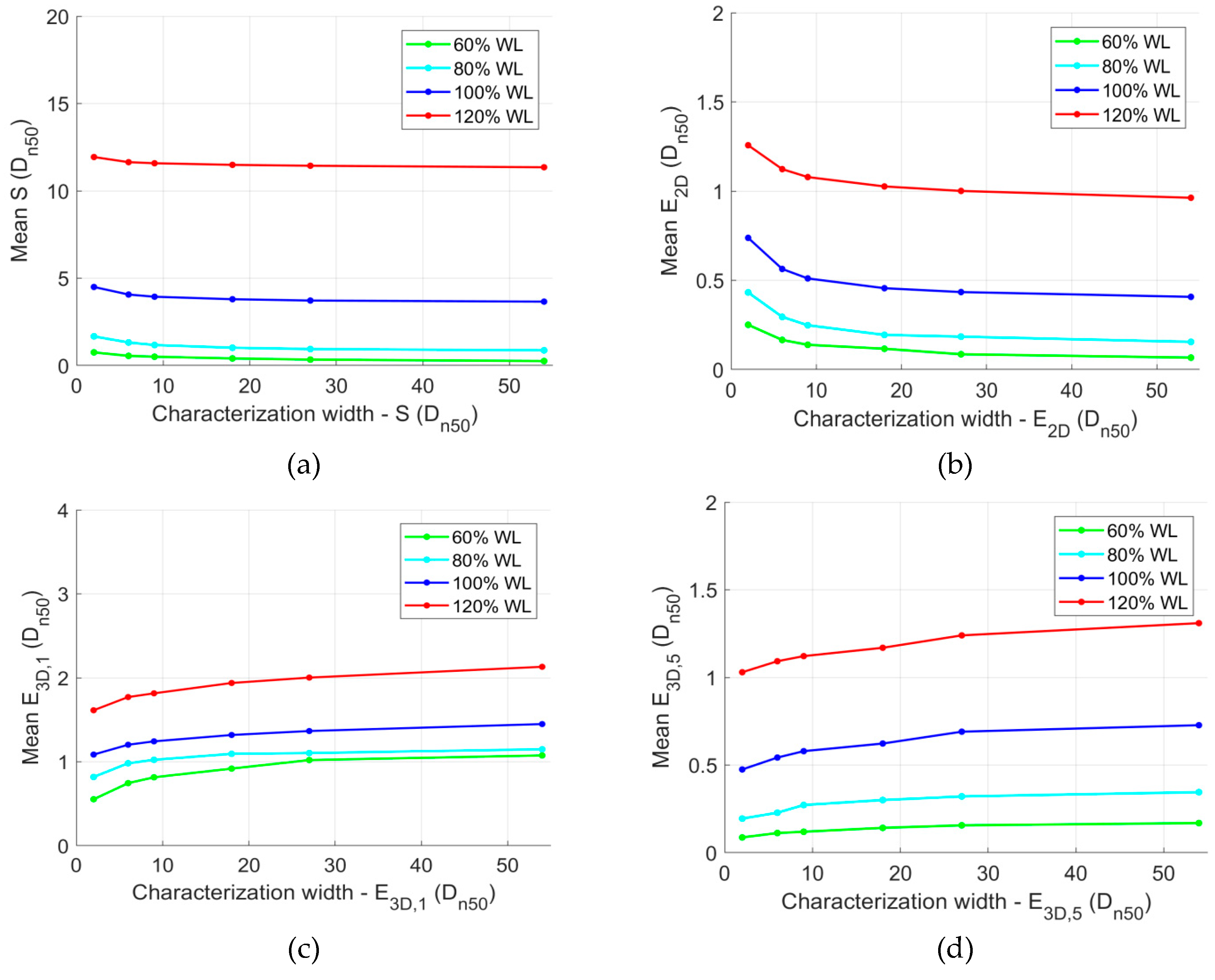Figure 7, Figure 8, and Figure 9 show, respectively, the mean damage values, the standard deviations, and the variations as a function of the width over which the damage was determined. These figures illustrate that the damage values were affected by the width over which the damage was determined. This is not only valid for the present tests, but for all physical model tests with rock slopes.

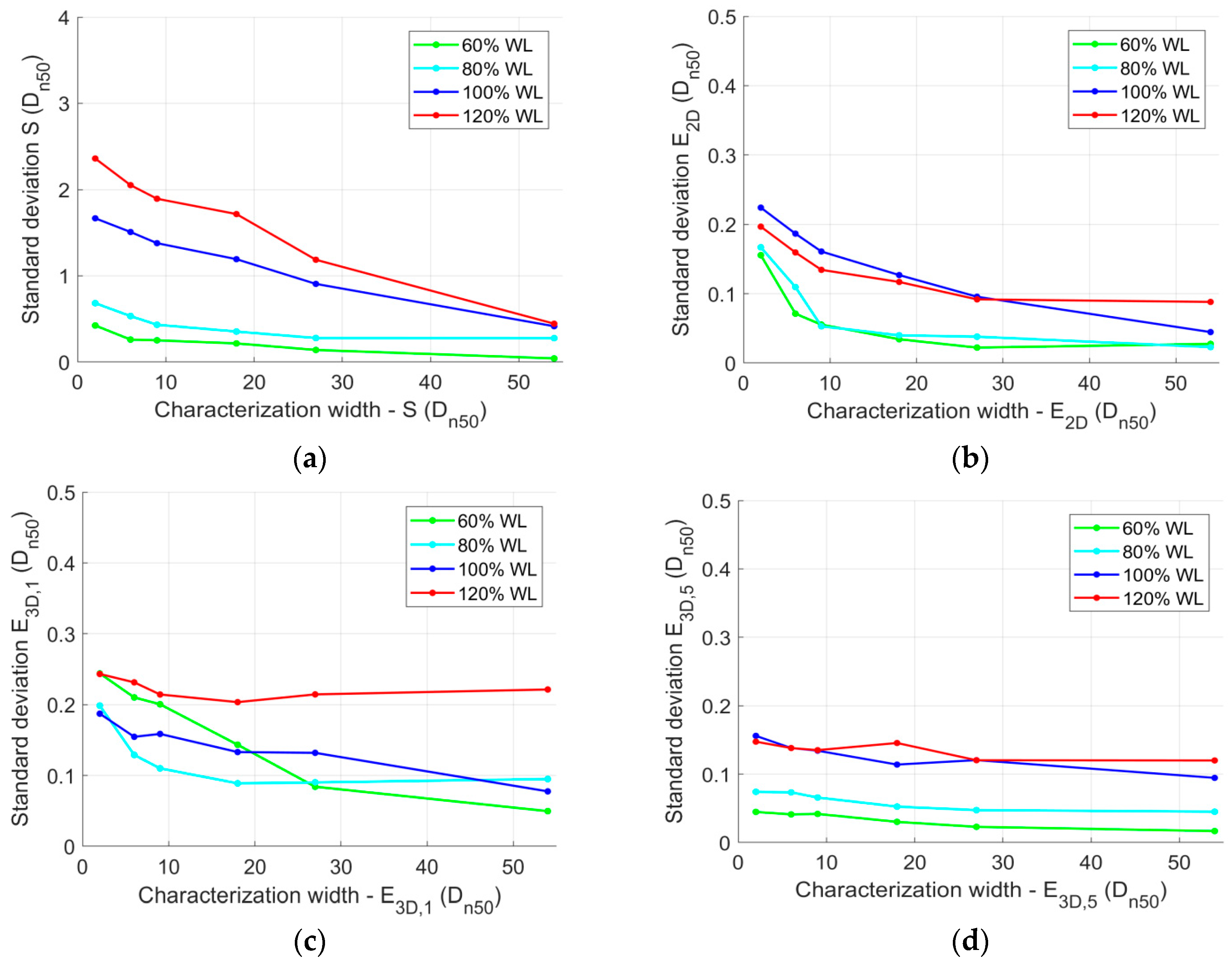
Figure 8 shows that the width over which the damage is obtained (i.e., the characterisation width) also affects the standard deviations of the damage parameters. Figure 8a shows that for the damage parameter, S, the standard deviations were highly affected by the width of the section over which the damage was determined. Figure 8b,d show that the standard deviations of the parameters, E_2D and E_3D,5, are more or less constant for a section with a width of 25 stones or more. Figure 8c shows that for the parameter, E_3D,1, there is not a clear trend; for some conditions, the values decrease for wider sections while for other conditions, the values are constant for wider sections.

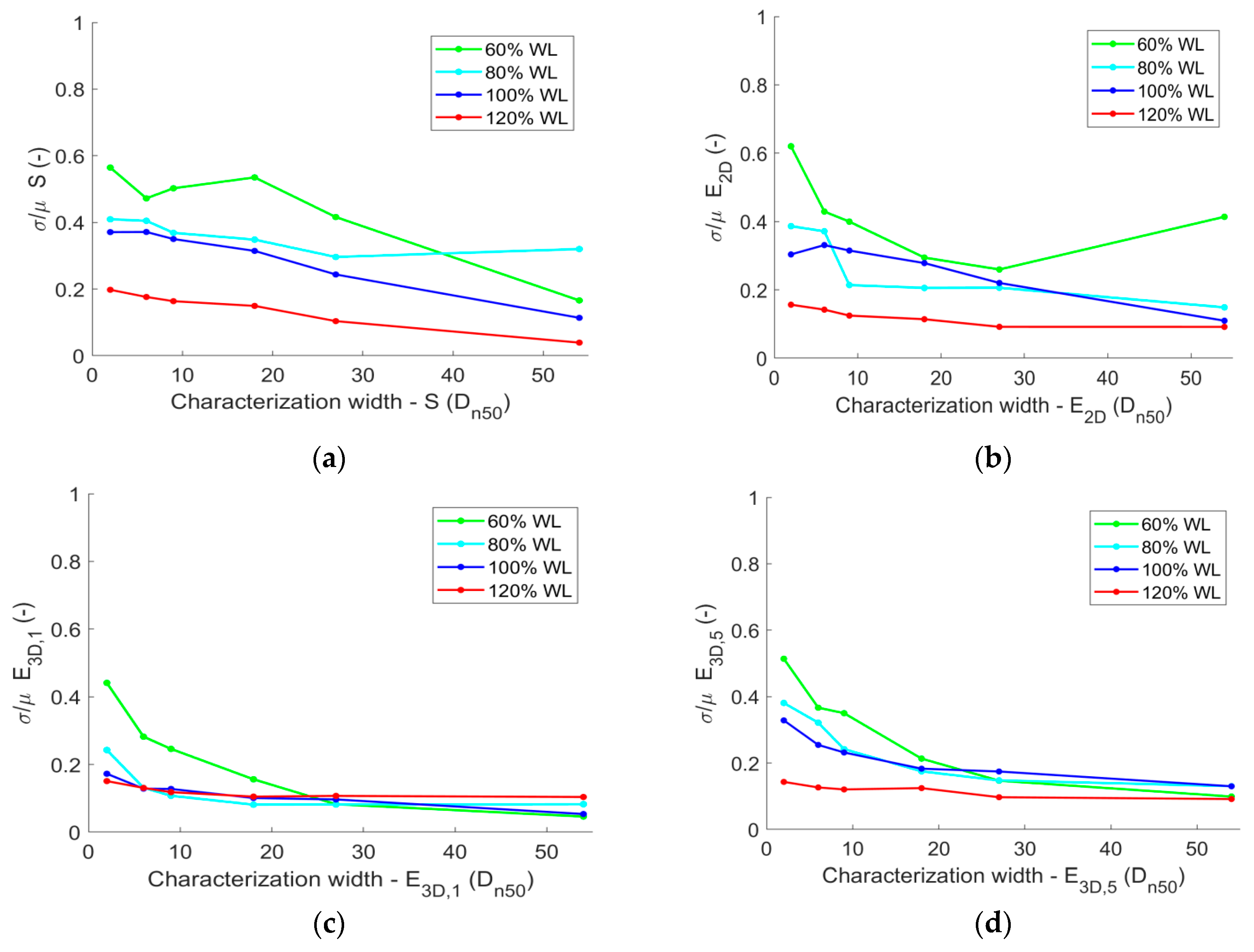
Figure 9 shows the variation as a function of the width over which the damage was obtained. For the lower damage values (i.e., at the 60% and 80% water levels), the variability of the damage parameters, E_3D,1 and E_3D,5, was less than for the damage parameters, S and E_2D. For the higher damage values (i.e., at the 100% and 120% water levels) and the largest width of the test section (e.g., a width of 54 stones), there was no clear difference between the variation values of the various damage parameters. Figure 9 shows that the variation of the damage parameters, E_3D,1 and E_3D,5, does not vary significantly for various widths over which the damage was obtained, as long as the width was about 25 stones or more. Note that for E_3D,1 and E_3D,5, the mean values increase for a larger width, such that for equal values of the spreading, the variations decrease for a larger width. As also discussed in [13,14], it is recommended that damage is determined in a wave flume over a width of about 25 stones.

Besides the width over which the damage was determined in the tests affecting the damage values, there is also a difference between the width of the structure in the tests (scaled to prototype) and the width of the structure in reality. The present tests can be used to take this effect into account. This is the so-called length effect and this will be discussed in the following section.

4. Length Effect

Damage is normally measured over a specific width in a wave flume (here, 54 stones of 0.0163 m). In reality, the width of the structure is likely to be longer than the width (scaled to prototype dimensions) applied in the tests. Therefore, the mean and maximum damage in the real structure can deviate from the mean and maximum damage measured in the tests. This is called the length effect of the structure. In this section, the subscript, m, refers to model test results and the subscript, p, refers to real (prototype) structures. Given that, in this study, tests have been repeated, the mean values and standard deviations of the damage can be determined. These can be used to extrapolate the results in a narrow section (i.e., the test section) to a wider section, the width of the real structure. Several assumptions are made in the following method of which the most important are that damage is normally distributed and that the spreading in the present tests is representative of other structures with rock slopes.

Due to the assumption that the damage is normally distributed, the probability that at any location within the test section the damage, S, is larger than the damage, S_m, obtained over the entire width of the measurement section is 50%, thus P(S > S_m) = 0.5 (S_m characterises the mean damage in the model test section since it is based on the averaged profile over the width of the test section). For practical situations in physical model tests, this is considered as a reasonable assumption for damage numbers of S_m ≥ 2. The probability that within this test section there is at any location damage that exceeds a pre-described critical damage, S_crit (i.e., the maximum allowable damage) is denoted by P(S > S_crit).

$$P(S_{}>S_{crit})=1-F(S_m)$$

(1)

where F (S_m) is the cumulative normal distribution, with the (mean) value, S_m, and standard deviation, σ, from the model tests (In Excel: F (S_m) = NORM.DIST (S_crit; S_m; σ; TRUE)).

To calculate the length effect due to the difference between the width of the test section, the scaled to prototype scale, L_m, and the width of the real structure, L_p, the ratio of these two, r = L_p/L_m, is used. The probability that in the real (prototype) structure a critical damage is exceeded at any location is:

$$P(S_p>S_{crit})=1-[F(S_m){]}^r$$

(2)

where F (S_m) is the same cumulative normal distribution, with the (mean) value, S_m, and the standard deviation, σ, from the model tests.

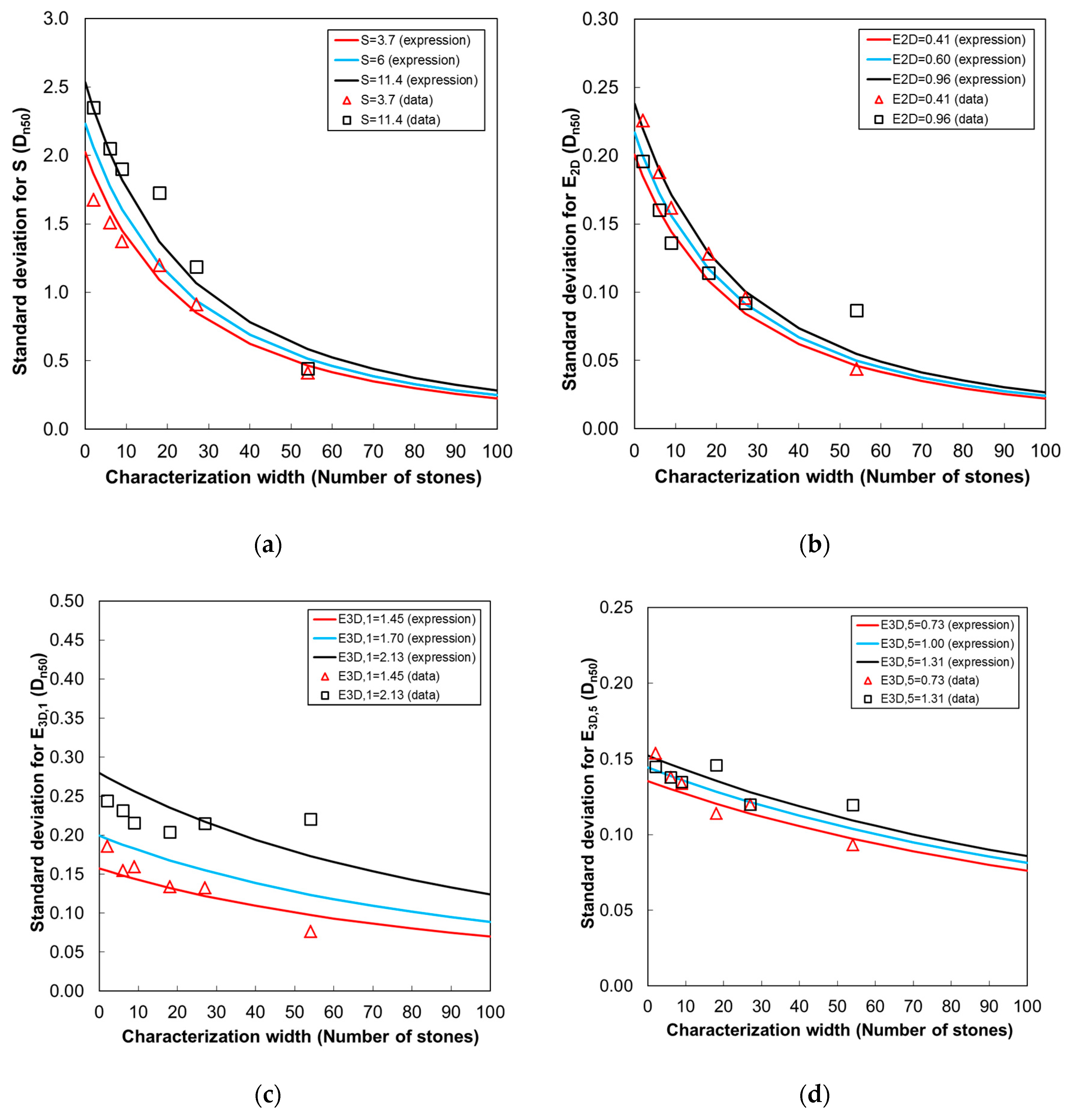
If a model test is performed without any repetitions, the standard deviation, σ, can be estimated based on the present tests. The standard deviation and variation (σ/μ, where μ = S_m) appeared to be dependent on the amount of damage and on the width of the test section (i.e., the number of stones, N_st, within the width of the test section). For the four different damage parameters’ standard deviations obtained from the tests (see Table 2 and Figure 8), a simple fit can be used for the damage levels between the start of the damage and failure (i.e., for S between 2 < S < 12). These fits are given in Equations (3a)–(3d) and Figure 10. Note that these expressions for the standard deviations include not only the damage level, but also the number of stone, N_st, within the width of the test section. The latter influence was not included in [10].

$$S:{\sigma }_{}=3900S_{}{}^{0.2}{\left(N_{st}+50\right)}^{-2}\mathrm{for}2\le S\le 12$$

(3a)

$$E_{\mathit{2}D}:{\sigma }_{}=600E_{2D}{}^{0.2}{\left(N_{st}+50\right)}^{-2}\mathrm{for}0.2\le E_{\mathit{2}D}\le 1.2$$

(3b)

$$E_{\mathit{3}D,\mathit{1}}:{\sigma }_{}=3600E_{3D,1}{}^{1.5}{\left(N_{st}+200\right)}^{-2}\mathrm{for}1.2\le E_{\mathit{3}D,\mathit{1}}\le 2.2$$

(3c)

$$E_{\mathit{3}D,\mathit{5}}:{\sigma }_{}=13000E_{3D,5}{}^{0.2}{\left(N_{st}+300\right)}^{-2}\mathrm{for}0.3\le E_{\mathit{3}D,\mathit{5}}\le 1.4$$

(3d)

Assuming that the standard deviations in the present tests are representative for all rock slopes, the above mentioned expressions for the probability that a critical value is exceeded can be used for other physical models representing real structures using only the parameters, r (for that particular structure), and the measured damage, S_m (for that particular test) and S_crit (for that particular structure in reality). The expressions relating the standard deviation to the amount of damage and the number of stones applied in the tests provide a robust estimation of the standard deviation. As can be seen in Table 2, the associated uncertainties in the estimates of the damage are large.

The width of the real (prototype) structure, L_p, can be divided into r sections with a (scaled) width of the test section, L_m. The average damage profile in each of these r sections provides r values of S_p. Analogous to what is being assumed in the test section, the probability that at any location the damage, S, is larger than the damage value of that section, S_p, is 50%, thus P(S > S_p) = 0.5. The maximum damage of the r values of S_p will be higher than the damage in the model, S_m. This maximum value (which is still a value based on an averaged profile over a width of L_m) can be calculated as follows:

$$S_p=F^{-1}\left({0.5}_{}{}^{\frac{1}{r}}\right)$$

(4)

where F^-1(S) is the inverse of the cumulative normal distribution, with the value, S_m, and standard deviation, σ, both from the model tests (In Excel: S_p = NORM.S.INV(0.5^(1/r)) σ + S_m).

The above expressions (Equations (1), (2), and (4)) can also be applied for the other mentioned damage parameters, but the expression to relate the standard deviation to the amount of damage varies per damage parameter (Equations (3a)–(3d)).

These expressions (Equations (3a)–(3d)) lead to variations (σ/μ) that decrease for larger damage values using S, E_2D, or E_3D,5 or increase for larger values using E_3D,1. Note that [6] also derived estimates of the spread depending on the amount of damage, but those were based on individual damage profiles and not on average damage profiles.

In the above described expressions, the assumption is made that the damage to the rock slope is normally distributed and consequently the maxima are Gumbel distributed. For all mentioned damage parameters, (S, E_2D, E_3D,1, and E_3D,5) Equations (1), (2), and (4) can be used. In contrast to the damage parameters, S and E_2D, that are based on average damage profiles, the damage parameters, E_3D,1 and E_3D,5, are based on maximal values that occurred over the width of the measurement section. Since the latter two are based on maxima, extreme value analysis can be used. To account for the difference between the width of the test section, scaled to the prototype scale, L_m, and the width of the real structure, L_p, the ratio of these two, r = L_p/L_m, can be used to determine the damage value in the real structure, using the Gumbel distribution:

$$E_{3D}={\mu }_G-{\sigma }_G\hspace{0.17em}\ln \left(-\ln \left(1-\frac{1}{r}\right)\right)$$

(5)

where μ_G and σ_G are the location and scale parameters of the Gumbel distribution, which can be computed directly from the mean (E_3D,m) and standard deviation (σ) obtained from the model tests using σ_G = σ 6^0.5/π and μ_G = E_3D,m − 0.577 σ_G.

To illustrate the importance of the length effect and taking into account the spreading of the results, an example is given here based on Equation 1 to 5 (bold are assumed input values; in italics, red is the outcome of this example).

L = Width of the test section in the model:	0.8 m
Dn50 = Stone diameter in the model (Nst = L/Dn50):	0.0125 m
M = Model scale:	50
Lm = Width of the test section scaled to prototype scale (m):	40 m
Lp = Width of the real (prototype) structure (m):	1000 m
R = Lp/Lm	25
Sm = Damage observed in model test (based on the average profile):	5
σ = Standard deviation of the damage, using Equation (3a) with S = Sm = 5:	0.414
Sp = Damage (maximum of r sections) in the real (prototype) structure, using Equation (4):	5.80
Scrit = Critical damage: Maximum allowable damage in the real (prototype) structure:	6
P(Sm > Scrit) = Probability that S at any cross-section in a model is larger than Scrit (Equation (1)):	0.008
P(Sp > Scrit) = Probability that S at any cross-section in the real structure is larger than Scrit (Equation (2)):	0.179

This example shows that for a model test with, for instance, a measured damage of S = 5, there is a probability of 17.9% that in the real structure, S = 6 will be exceeded while the probability that S = 6 will be exceeded in the tests is less than 1%. The damage value for the real structure (i.e., the maximum damage based on a damage profile averaged over a width of 40 m in the real structure: The maximum value of 1000 m/40 m = 25 damage values) will be higher than the damage in the model (i.e., the damage obtained based on the average profile in the measurement section): 5.80 versus 5.

In above described example, the damage parameter, S, was used, but the same can be done for the other three damage parameters, using the earlier mentioned expressions for the standard deviation, σ, for each damage parameter.

The following example provides an illustration of the length effect using another damage parameter, namely E_3D,5.

E3D,5-m = Damage observed in model test (based on the average profile):	0.60
σ = Standard deviation of the damage, using Equation (3d) with E3D,5 = 0.60:	0.09
E3D,5-p = Damage in the real (prototype) structure, using Equation (4) (Normal distribution):	0.770
E3D,5-p = Damage in the real (prototype) structure, using Equation (5) (Gumbel distribution):	0.781
E3D-crit = Critical damage: Maximum allowable damage in the real (prototype) structure:	0.8
P(E3D,5-m > E3D-crit) = Probability that E3D,5 in a model is larger than E3D-crit (Equation (1)):	0.012
P(E3D,5-p > E3D-crit) = Probability that E3D,5 in the real (prototype) model is larger than E3D-crit (Equation (2)):	0.260

This example shows that for a model test in which a damage level of E_3D,5 = 0.60 is measured, there is a probability of 26% that in the real structure, that is 25 times wider (R = L_p/L_m = 25), the critical value of E_3D,5 = 0.80 will be exceeded. The damage in the real structure will be higher than the measured damage in the model; in the case when a normal distribution is used, E_3D,5 = 0.77 versus E_3D,5 = 0.60, while in the case when the Gumbel distribution is used, E_3D,5 = 0.78 versus E_3D,5 = 0.60. Thus, in this example, the expected damage values for the real (prototype) structure are not sensitive to the applied approach; for both distributions, the expected damage values, E_3D,5, in the real structure are similar and are clearly larger than that observed in the measurements.

In the approach described here, the measured spreading in Series S1 was considered as representative, rather than Series S2. In Series S1, milder wave conditions were generated prior to the design condition (100% WL). This is considered as being more representative of real structures since before reaching the peak of the storm (that is modelled in the model tests), milder wave conditions also occur earlier in a storm. In addition, it is likely that structures experience storms prior to the design storm. In Series S2, no milder conditions were present prior to the design condition. Therefore, the standard deviations in the above-mentioned approach are based on Series S1 and not on Series S2. Note that, unlike the spreading, the mean damage values obtained in Series S1 and Series S2 are rather similar.

5. Conclusions and Recommendations

Based on the physical model tests, the damage to rock armoured slopes was analysed for conditions with different water levels in still water. The wave conditions in deep water were the same, but due to the shallow foreshore, the wave conditions at the base of the structure varied considerably. Tests with a straight slope and tests with berms were performed. Those with a straight slope were performed five times and this allowed for an analysis of the spreading in the tests results. The following conclusions can be drawn based on the described study:

• Increasing water levels can increase the damage to rock armour slopes considerably for structures with a shallow foreshore. In the performed tests, the increasing water levels caused increased wave loading and consequently an increase of the damage with a factor 2 (for E_3D,1) to 44 (for S) while the wave conditions in deep water were equal. Thus, this factor depends on which parameter is used to characterise the damage.
• Wide berms (with a width of 10 stone diameters) are effective to reduce the total damage to the armour layer, irrespective of the parameter that is used to characterise the damage. Berms can be added to existing straight slopes to reduce overtopping and damage from increasing water levels and increasing wave loading without increasing the crest level. Since the level of berms can be increased relatively easily once sea water levels increase, adding and/or modifying a berm is a useful measure for climate adaptation.
• The present tests can be used to estimate the spreading of the damage to rock armoured slopes for tests that have not been repeated as many times as in the present tests. Simple expressions were derived to estimate the standard deviations and variations in the damage to rock armoured slopes.
• With the range of damage that is normally considered relevant, 2 < S < 12 (where S = 2 is characterised as the start of the damage and S = 12 as failure for the tested 1:3 slope), the variations in the damage values are comparable for the various damage parameters (S, E_2D, E_3D,1, and E_3D,5). However, for the tests without milder conditions prior to the design condition (i.e., 100% water level in Series S2), the variations in the damage parameters, E_3D,1 and E_3D,5, are clearly less than for the damage parameters, S and E_2D.
• If conditions with lower waves precede the design conditions, the magnitude of the damage is similar to the situation where no conditions with milder waves precede the design condition. However, the variability in the damage increases if no conditions with milder waves precede the design condition.
• Since in 2D physical model tests, structures are generally less wide than the real (prototype) structures that they resemble, the difference between the scaled width of the structure in the model and the width of the structure in reality needs to be taken into account. Expressions to take this length effect into account were proposed.

Since the spreading of the damage to rock armoured slopes is rather large, future research should aim to study the spreading of the damage to rock armoured slopes in more detail with even more repetitions than performed here. It is recommended to take the spreading of the damage to rock armoured slopes into account in physical model tests and in reality; in investigations where only one test is performed, the presented tests can provide an estimate of the spreading. It is recommended that the length effect is considered if the structure, in reality, is wider than the scaled width of the model in a wave flume.