All articles published by MDPI are made immediately available worldwide under an open access license. No special
permission is required to reuse all or part of the article published by MDPI, including figures and tables. For
articles published under an open access Creative Common CC BY license, any part of the article may be reused without
permission provided that the original article is clearly cited. For more information, please refer to
https://www.mdpi.com/openaccess.
Feature papers represent the most advanced research with significant potential for high impact in the field. A Feature
Paper should be a substantial original Article that involves several techniques or approaches, provides an outlook for
future research directions and describes possible research applications.
Feature papers are submitted upon individual invitation or recommendation by the scientific editors and must receive
positive feedback from the reviewers.
Editor’s Choice articles are based on recommendations by the scientific editors of MDPI journals from around the world.
Editors select a small number of articles recently published in the journal that they believe will be particularly
interesting to readers, or important in the respective research area. The aim is to provide a snapshot of some of the
most exciting work published in the various research areas of the journal.
Methods for the separation of long-crested linear waves into incident and reflected waves have existed for more than 40 years. The present paper presents a new method for the separation of nonlinear bichromatic long-crested waves into incident and reflected components, as well as into free and bound components. The new method is an extension of a recently proposed method for the separation of nonlinear regular waves. The new methods include both bound and free higher harmonics, which is important for nonlinear waves. The applied separation method covers interactions to the third order, but can easily be extended to a higher orders. Synthetic tests, as well as physical model tests, showed that the method accurately predict the bound amplitudes and incident and reflected surface elevations of nonlinear bichromatic waves. The new method is important in order to be able to describe the detailed characteristics of nonlinear bichromatic waves and their reflection.
In physical model tests, it is very important to know in detail the wave conditions that are present in the facility. Incident waves hit passive or active absorbers or structures and are partly absorbed and partly reflected. Thereafter, the wave system includes both incident and reflected components. Nonlinear waves might at a given frequency include both bound and free components, making the separation into incident and reflected components more complicated. In regular or bichromatic waves, free incident higher harmonics are usually unwanted, as they mainly exist if the bound components were not correctly generated by the wave maker. Moreover, in regular and bichromatic waves, the bound harmonics at a given frequency usually stem from only one interaction. In irregular waves, this is not the case, and moreover, for wider spectra the primary energy overlaps with the sub- and superharmonics. If the wave height decreases, for example due to wave-breaking or waves propagating into deeper waters, the generation of free harmonics might also occur.
The present paper presents a detailed analysis of two-dimensional model tests with unidirectional bichromatic waves. Bichromatic waves are commonly used for detailed studies on the effect of bound sub- and superharmonics on, for example, the response of beaches and structures. Therefore, being able to accurately separate these waves into incident and reflected as well as bound and free components is of high interest.
Historically, waves have been separated into incident and reflected components based on methods assuming linear waves, cf. Goda and Suzuki [1], Mansard, and Funke [2], and Zelt and Skjelbreia [3]. Today, these methods are standard tools used in most hydraulic laboratories, but these methods do not consider any bound components to be present and also disregard amplitude dispersion. The few existing methods for nonlinear waves use questionable assumptions, e.g., the Lin and Huang [4] method, which applies to regular waves but disregards amplitude dispersion and thus is only applicable to mildly nonlinear regular waves. The nonlinear LASA methods (Local Approximation using Simulated Annealing) by Figueres et al. [5] and Figueres and Medina [6] are based on local time domain solutions fitted to theoretical wave profiles, making application of their method to cases where free energy exists questionable. Even when no free energy exists and even for linear waves, Lykke Andersen et al. [7] and Eldrup and Lykke Andersen [8] found that the LASA V method was not accurate, and as the method at the same time is computationally very expensive, it is not practical for real applications.
Recently, a nonlinear frequency domain method to separate regular waves into incident and reflected components was developed, cf. Lykke Andersen et al. [7]. This method is an extension of the Lin and Huang [4] method, but includes amplitude dispersion based on stream function wave theory (Fenton and Rienecker [9]). This nonlinear separation method was further extended by Eldrup and Lykke Andersen [8] to irregular waves by utilizing a narrow-band assumption for the primary spectrum. They showed that even for typical single-peaked primary spectra (JONSWAP with γ = 3.3), this assumption was leading to accurate estimated incident and reflected waves even for highly nonlinear waves. The reason for this was that the main contribution to the bound superharmonics stems from the interaction of components near the peak frequency of the primary spectrum.
The narrow-band assumption applied by Eldrup and Lykke Andersen [8] for the separation of irregular waves is not necessarily valid for nonlinear bichromatic waves if the frequency interval between the two primary components is not small enough. However, as the bound waves in bichromatic waves normally stem mainly from only one interaction, a more accurate method could be developed. Such a method is presented in the present paper, and the new method is evaluated on new model tests performed in a wave flume at the Atmosphere-Ocean Interaction Flume in Granada, Spain.
2. Third-Order Wave Theory for Bichromatic Waves
Bichromatic waves refer to waves with two primary incident components at cyclic frequencies ωn and ωm. The surface elevation of such incident waves can, with first-order theory, be expressed as
Second-order theory for a bichromatic group gives additionally three bound superharmonic components (sum-interactions) at the cyclic frequencies 2ωn, 2ωm, and ωn + ωm, and one subharmonic component (difference-interactions) at cyclic frequency ωm − ωn (assuming ωm > ωn). Complete expressions, including second-order transfer functions (G), are given in, for example, Sharma and Dean [10], Schäffer [11], and Madsen and Fuhrman [12,13]. The second-order contribution due to the interaction of component n and m can be written as:
This gives one subharmonic contribution (ηn−m) and three superharmonic contributions (η2n, η2m, ηn+m). The period of the subharmonic component (T = 2π/(ωm − ωn)) also corresponds to the duration of the formed wave group. A correction to the linear dispersion equation appears first at third order, and thus in second order theory the linear dispersion equation is valid for the primary components. The wave numbers of the bound superharmonics are calculated as the sum of the wave numbers of the interacting components and the difference for the subharmonics. Thus, the celerity of the bound components due to interaction of component n and m can be calculated as cn−m = (ωm − ωn)/(km − kn) for the subharmonic and cn+m = (ωm + ωn)/(km + kn) for the superharmonic component.
Recently, third-order solutions for bichromatic waves as well as for irregular waves were developed, cf. Madsen and Fuhrman [12,13]. Applying that theory to unidirectional bichromatic waves yields additionally four bound superharmonic components at the cyclic frequencies 3ωn, 3ωm, ωm + 2ωn, ωn + 2ωm and two additional bound subharmonics at the cyclic frequencies |ωn − 2ωm| and |ωm − 2ωn|. The computational cost of that method for irregular waves is very high, but for bichromatic waves the computational cost is very small. The wave numbers of the bound waves at the above given angular frequencies are found simply by summation and differences of the wave numbers for the primary frequencies (as in the second-order components given in Equation (2)). Thus, for example, the wave number of the bound component at frequency ωm + 2ωn is given by km + 2kn. The celerity of the bound components can afterwards be calculated using the same principle as for the second-order components. However, the celerity of the primary components is different from the first-order values due to amplitude dispersion. The dispersion equation was derived to third order by Madsen and Fuhrman [12,13]. Here, it was shown that the celerity of each of the two primary components depend on the amplitude and frequency of both components.
3. Nonlinear Reflection Separation Method for Bichromatic Waves
Lykke Andersen et al. [7] showed that for regular waves the celerity of the bound superharmonics is higher than a free component at the same frequency, and this makes it possible to separate the bound and free waves. The same applies to bichromatic waves, and thus for bichromatic waves it is also possible to separate the bound and free superharmonic components due to their different celerities. The bound subharmonic component has a lower celerity than a free one at the same frequency. Thus, it is also possible to separate these components based on their differences in celerity. However, for shallow water waves, the celerities of the bound and the free waves are almost identical, and thus separation of the two is not possible.
The mathematical model used for the separation of nonlinear bichromatic waves is chosen as a third-order surface for the incident as well as for the reflected waves. Moreover, free incident and reflected components are included in all of the sub- and superharmonic frequencies. Finally, a noise term (Ω) is included. In the following, it is assumed that at the frequencies of the two primary components, only primary incident and reflected waves exist. In special cases, it might occur for bichromatic waves that the frequency of one or more of the sub- or superharmonic components is coincident with either a primary component or another higher harmonic. This is a special case that for the moment is not covered by the present method. For irregular waves, this occurs to a large extent, and Eldrup and Lykke Andersen [8] used a narrow band assumption for the primary spectrum to overcome this issue.
In order to separate the bichromatic waves, a mathematical model for the surface is needed at every frequency present in the signal. The surface is expressed at each of the wave gauges (xj) in the frequency domain (Fourier space). The signal include both incident and reflected waves, and due to amplitude dispersion, the wave numbers are different for the incident waves (kn,I, km,I) and the reflected (kn,R, km,R) primary components. Based on Equation (1) the following mathematical model is obtained at the two primary frequencies (where index i can take the values n and m and thus represent frequencies ωn and ωm):
where Δxj = xj − x1 is the distance between wave gauge number j and wave gauge number 1, i is the imaginary unit (i2 = −1), and Ωi,j is the noise at frequency ωi at gauge j. Later, an iterative procedure to estimate the wave numbers will be presented. The amplitudes are then calculated by a least-squares approach identical to that used by Lykke Andersen et al. [7] for regular waves.
Seven superharmonic frequencies (2ωn, 2ωm, ωm + ωn, 3ωn, 3ωm, ωm + 2ωn, ωn + 2ωm) and three subharmonic frequencies (ωm − ωn, |ωn − 2ωm| and |ωm − 2ωn|) are analyzed. These corresponded to the second- and third-order interaction frequencies given in Section 2. In the following, these frequencies are termed ωi, where index i can take the values 2n, 2m, m + n, 3n, 3m, m + 2n, m − n, n − 2m, and m − 2n. The related wave numbers of the bound wave are termed ki: For example, i = m + 2n corresponds to the cyclic frequency ωm + 2ωn, and the wave number of the bound wave is ki = km+2n = km + 2kn. These wave numbers are different for the incident and the reflected waves due to different primary wave numbers due to amplitude dispersion (kn,I, km,I for incident and kn,R, km,R for reflected). For these ten frequencies, the mathematical model consists of both free and bound components in the incident and reflected wave direction. The mathematical model can be written in frequency domain as
where kf is the wave number of the free waves at the cyclic frequency ωi and is calculated by the linear dispersion equation. The amplitudes of the bound harmonics can also be calculated by a least-square method when the wave numbers are known (see solution in Lykke Andersen et al. [7]).
Including terms up to the third order is reasonable for the tests considered in the present paper. Nevertheless, it is straightforward to extend the method to a higher order by applying Equation (4) at these frequencies. However, it is important to stress that it is assumed that only one (significant) bound interaction must occur at each frequency. This becomes more difficult to fulfill the higher order the waves are.
The wave numbers of the two primary components determine the wave numbers of each of the bound sub- and superharmonics analyzed with Equation (4). Thus, a critical part of being able to separate accurately the bound and the free harmonics is to have an accurate estimate of the wave number (or the celerity) of the two incident and reflected primary components that the bichromatic waves consist of. In principle, these four wave numbers could be unknown parameters in the mathematical model to be calculated, which, however, would result in nonlinear equations. Alternatively, they might be estimated by a wave theory, which was the procedure chosen by Lykke Andersen et al. [7] and Eldrup and Lykke Andersen [8] and which was also chosen for the present paper. In the present case, the wave numbers of the free sub- and superharmonic components (kf) were calculated with the linear dispersion equation. The wave numbers for the primary may be calculated with the third-order theory of Madsen and Fuhrman [12,13], which is valid for all of the present cases except one test (see Chapter 5). Initial tests showed that the presence of a second primary component did not influence significantly the celerity of the other component. Therefore, another possibility is to calculate the celerity of each primary component based on the stream function theory for regular waves by Fenton and Rienecker [9], with the parameters of each of the primary waves. This might increase the range of applicability to more shallow water waves. For the present test cases, the results were almost identical for the two methods, and thus more nonlinear waves in shallow water are needed to clarify this. The iterative procedure used is as follows:
Calculate the wave number for each primary frequency (n,m) based on linear dispersion, i.e., for infinitesimally small amplitudes of the primary components. Use this estimate as a starting guess for the incident and reflected wave numbers (kn,I, km,I, kn,R, and km,R);
Calculate first- to third-order incident and reflected components by applying the Lykke Andersen et al. [7] method on Equation (3) for the two primary frequencies and Equation (4) for the frequencies of the ten bound second and third harmonics. For bound components, use the latest estimated incident and reflected wave numbers (kn,I, km,I, kn,R, and km,R) calculated in either step 1 for the first iteration or step 3 for the following iterations. Free components are normally of much smaller height, and linear assumption is assumed valid for those;
Calculate updated values of kn,I, km,I, kn,R, and km,R either based on either a) third-order wave theory using the found amplitudes of the primary components, or b) ignoring the interaction of the two primary components (n and m), and thus a method for highly nonlinear regular waves can be applied for each component (e.g., stream function theory from Fenton and Rienecker (1980));
Repeat steps 2 and 3 until convergence is obtained for the incident and reflected wave numbers.
In principle, the calculations of the wave numbers should take into account the generated return currents from the incident and reflected waves. The third-order dispersion equation given by Madsen and Fuhrman [12,13] makes it possible to calculate the influence of the return currents on the celerities. This was done by calculating the celerities when no return currents were considered (U = 0) and when a closed basin was considered and thus a return current from the incident waves existed (q = 0). As the reflected waves generate a return current in the opposite direction, these calculations show the maximum influence of the return currents. For the test cases considered in the present paper, the difference on the celerities between using U = 0 and q = 0 was found to be from 0.2% to 0.9%, and thus the return current was not very important to include for the present tests. Therefore, it was decided to use U = 0 in the calculations, which was in line with what was used by Lykke Andersen et al. [7] for regular waves.
Moreover, the interaction of the incident and reflected waves was ignored, which from second-order wave theory is known to be a reasonable approximation (Eldrup and Lykke Andersen [8]). When both free and bound waves are present at a given frequency, this causes a modulation of the amplitude of the other components. This effect is mainly relevant when the bound and the free waves are high and have amplitudes of the same order of magnitude. This effect was not included in the mathematical model by Lykke Andersen et al. [7] and Eldrup and Lykke Andersen [8], and it was also ignored in the present paper.
Equations (3) and (4) are of similar form to the equations provided by Lykke Andersen et al. [7] for regular waves. Their solution can thus be applied also to bichromatic waves. Cases where the celerity of the free and the bound waves are almost identical can also be handled in a similar way to that presented in that paper. In bichromatic waves, the two primary frequencies in the signal would normally be known from the input to the wave maker. If this is not the case, a frequency domain analysis can be carried out to identify the frequency of the two highest peaks.
4. Validation on Synthetic Data
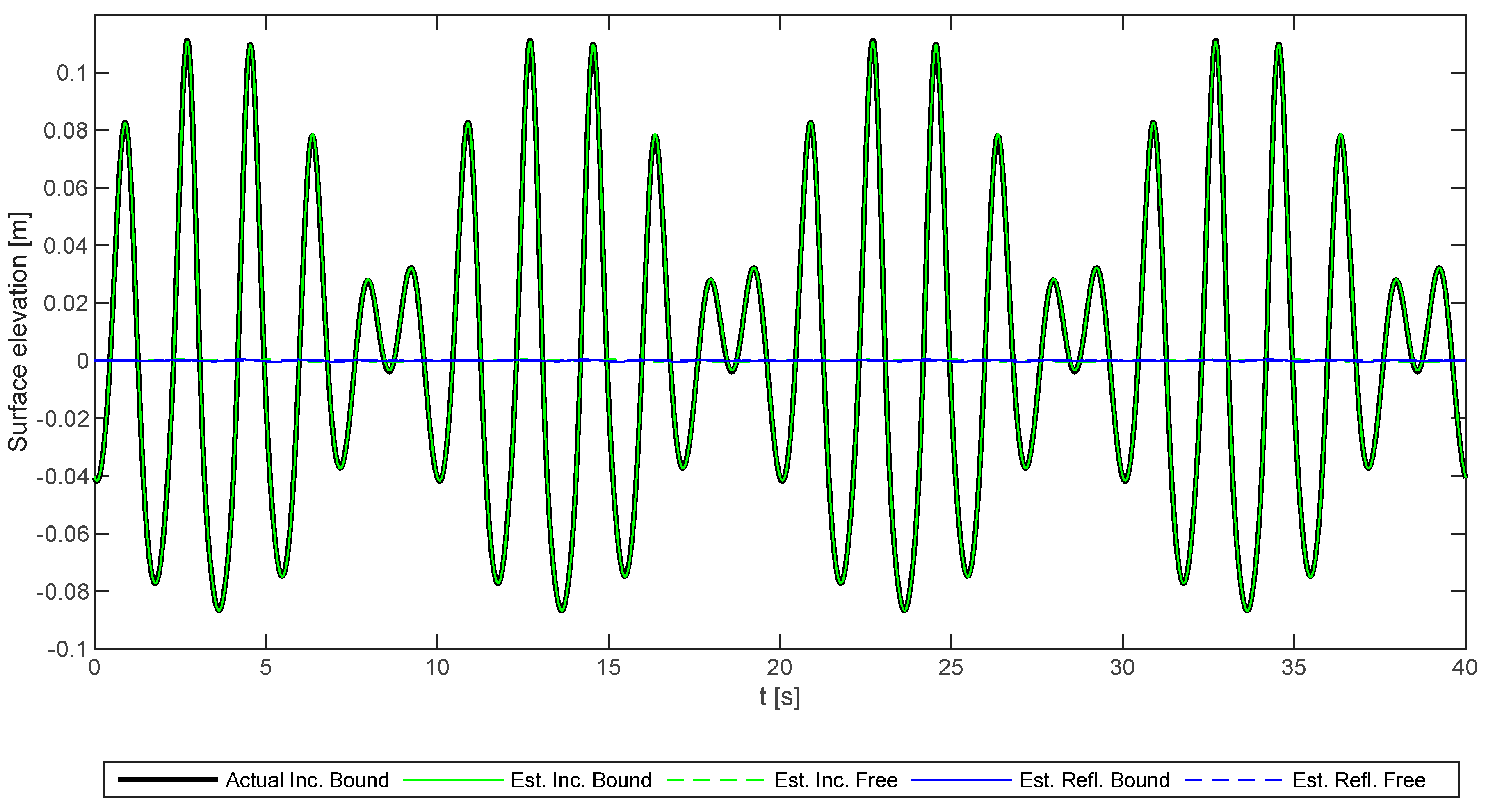
In order to validate the method and its implementation, bichromatic synthetic data were generated using the third-order theory of Madsen and Fuhrman [12,13]. The test case corresponds to “Test No. 2” in the later presented physical model tests (see Section 5). The data does not include any reflection or free harmonics. The wave gauge array used is also identical to that used in the physical model tests. The chosen phases of the two primary components are zero at x = 0.
Table 1 presents the actual amplitudes and the estimated ones. Note that there is almost full agreement, and errors on the amplitudes are typically less than 1%. Moreover, the estimated reflected free and bound components as well as the incident free components are close to zero, as used in the synthetic data. Minor errors are present mainly in the second-order components and are expected to be caused by small errors on the estimated celerities of the bound waves due to using third-order theory with q = 0 in the synthetic data and using stream function theory with U = 0 for each primary wave in the analysis method.
Additionally, the time series are plotted in Figure 1, which demonstrates that phases are also correctly calculated. Moreover, the figure gives an overall impression of the accuracy, as the estimated incident time series including only bound higher harmonics is almost identical to the target. Moreover, the estimated incident free higher harmonics, as well as the reflected components, are insignificant. Therefore, the implemented method was validated for data, fulfilling the assumptions of the method.
5. Physical Model Test Setup and Methodology
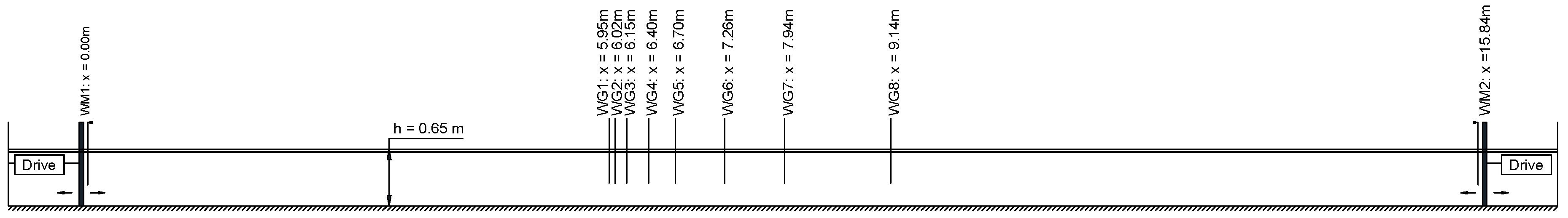
In order to evaluate the method, 2-D model tests were performed in a wave flume at the Atmosphere-Ocean Interaction Flume in Granada, Spain. The flume has a piston wave maker in each end, where one wave maker (WM1) is generating and absorbing waves, and the other wave maker (WM2) is only absorbing. The active absorption method used was the one presented by Lykke Andersen et al. [14], and the model test setup was also identical. An array of eight wave gauges (WG1–WG8) were used to test the above given reflection separation method. The method uses data from all gauges to calculate incident and reflected wave train components (amplitudes and phases). Based on the calculated components, the incident and reflected wave trains can be calculated at any point, but any errors in the mathematical model (for example, celerities) will amplify with distance from the central part of the wave gauge array. In the present paper, the time series will only be presented for x = 5.95 m (at the location of WG1). The water depth was constant throughout the length of the flume and equal to 0.65 m in all tests. The model test setup is shown in Figure 2.
Bichromatic waves were generated using the second-order wave maker theory of Schäffer [11], which correctly generates the bound sub- and superharmonics to second-order and thus minimizes free second-order incident energy. The test was performed for 240 s with a 10-s ramp up and down in each end. The analyzed part of the tests was from 40 s to 230 s. Table 2 presents the test conditions. With the chosen test conditions, the assumption in the mathematical model of all the primary and the interaction terms occurring at independent frequencies up to the third order was fulfilled. After Test Nos. 3, 8, and 9, some minor cross-modes were observed.
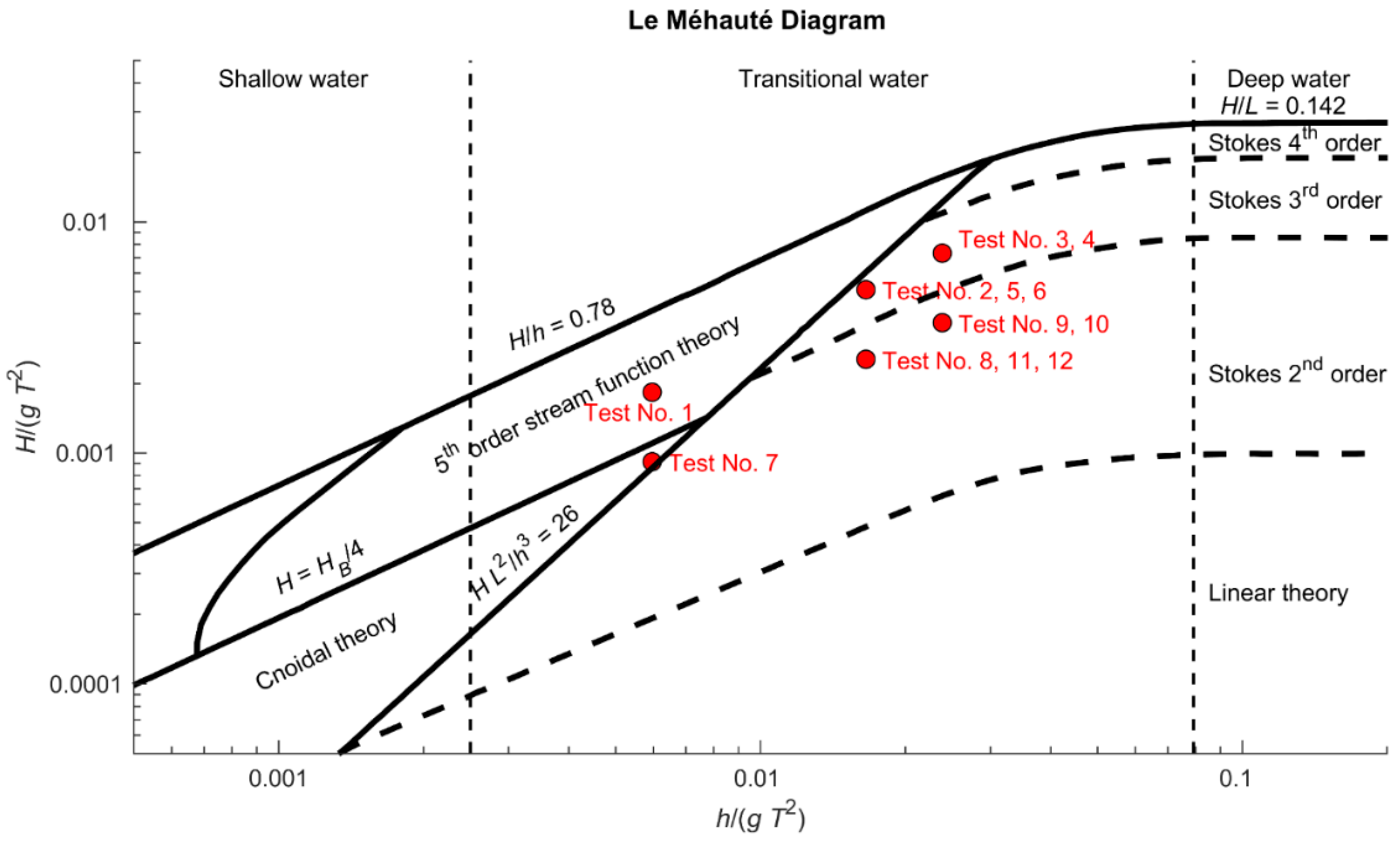
Figure 3 presents the test conditions in a Le Méhauté [15] diagram, where the data are plotted with the highest period of the two primary components and with the sum of their wave heights. In that way, the diagram should be slightly on the safe side with respect to the valid theory. It appears that third-order theory should be valid for all cases except for Test No. 1.
6. Physical Model Test Results
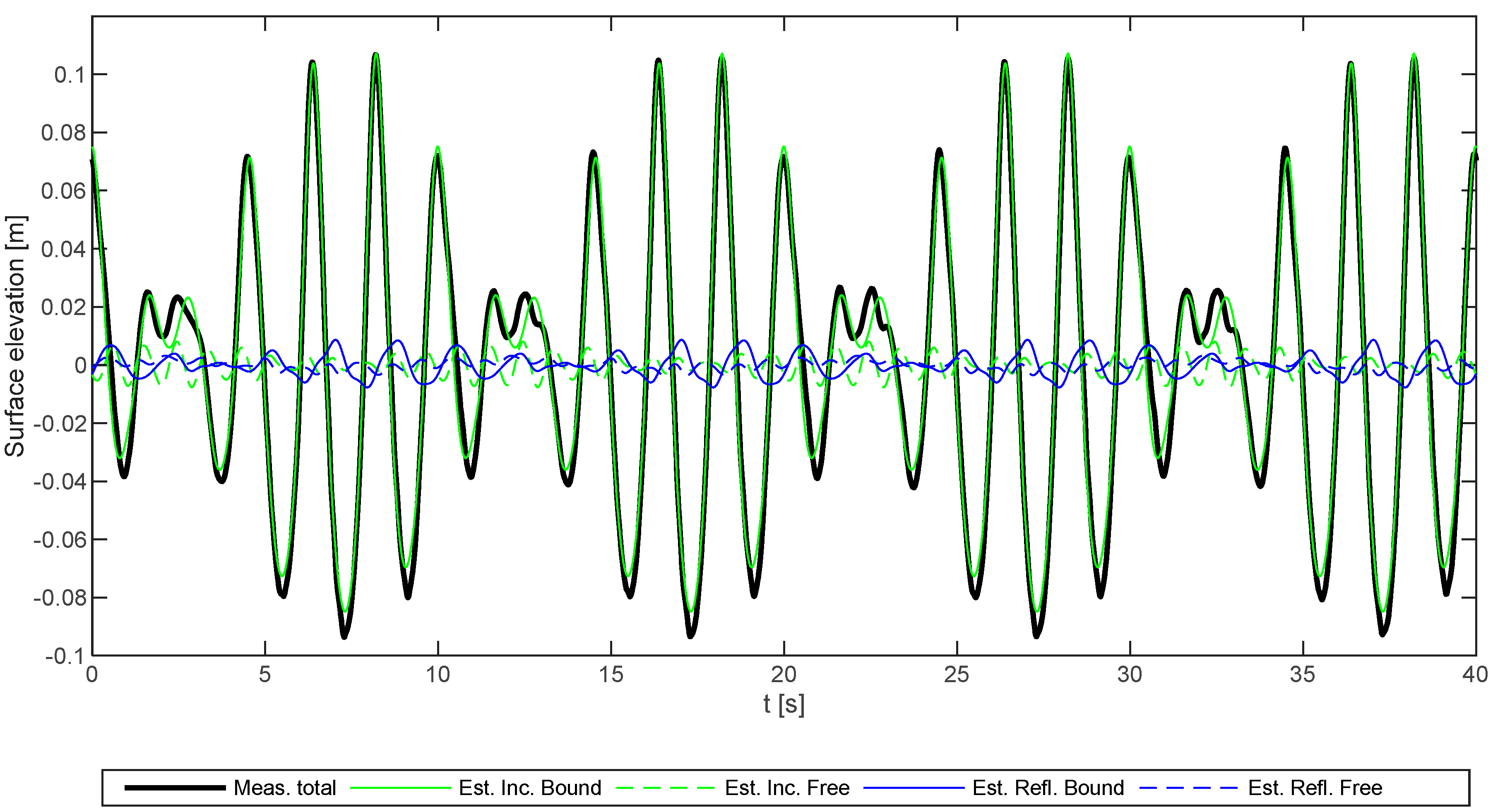
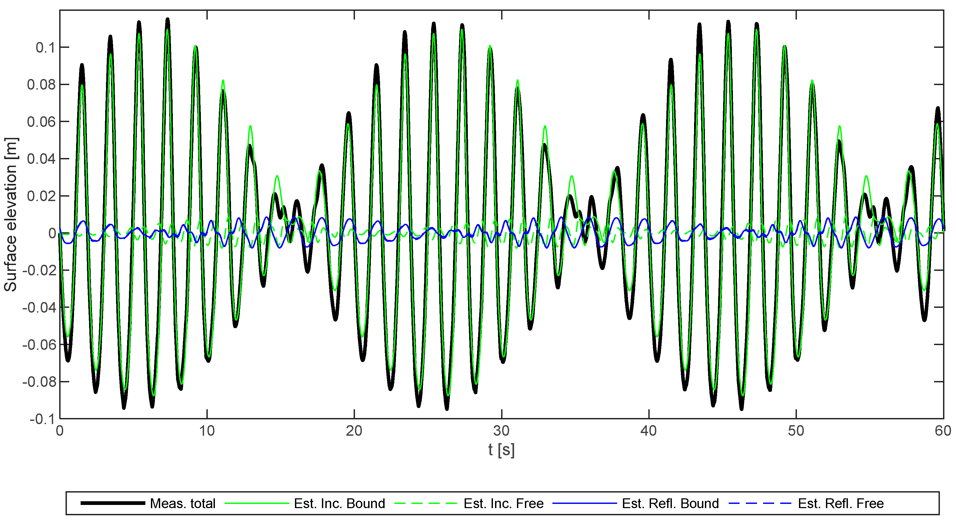
Figure 4 and Figure 5 show the incident and reflected time series for Test Nos. 2 and 5, respectively. The time series for the bound waves also include the two primary components. It appears that reflection is limited and in both cases at the order of 5%–10% of the incident wave. In the following, the focus is on analyzing the incident waves. An in-depth analysis of the reflection of the bound and free waves and a comparison to the linear absorption curve given by the Lykke Andersen et al. [14] method, is covered in detail by Lykke Andersen et al. [16].
Incident free waves of small amplitude are present, indicating that the bound harmonics were not generated accurately. This was maybe expected, as second-order generation was used while third-order theory was needed, according to Figure 3.
Table 3 presents the measured components for all the test cases using the present method. It appears that the two primary amplitudes are usually slightly lower than the target. This might be partly caused by energy needed to be stolen for the third-order components that were not generated and partly due to other issues such as leakage around the paddle.
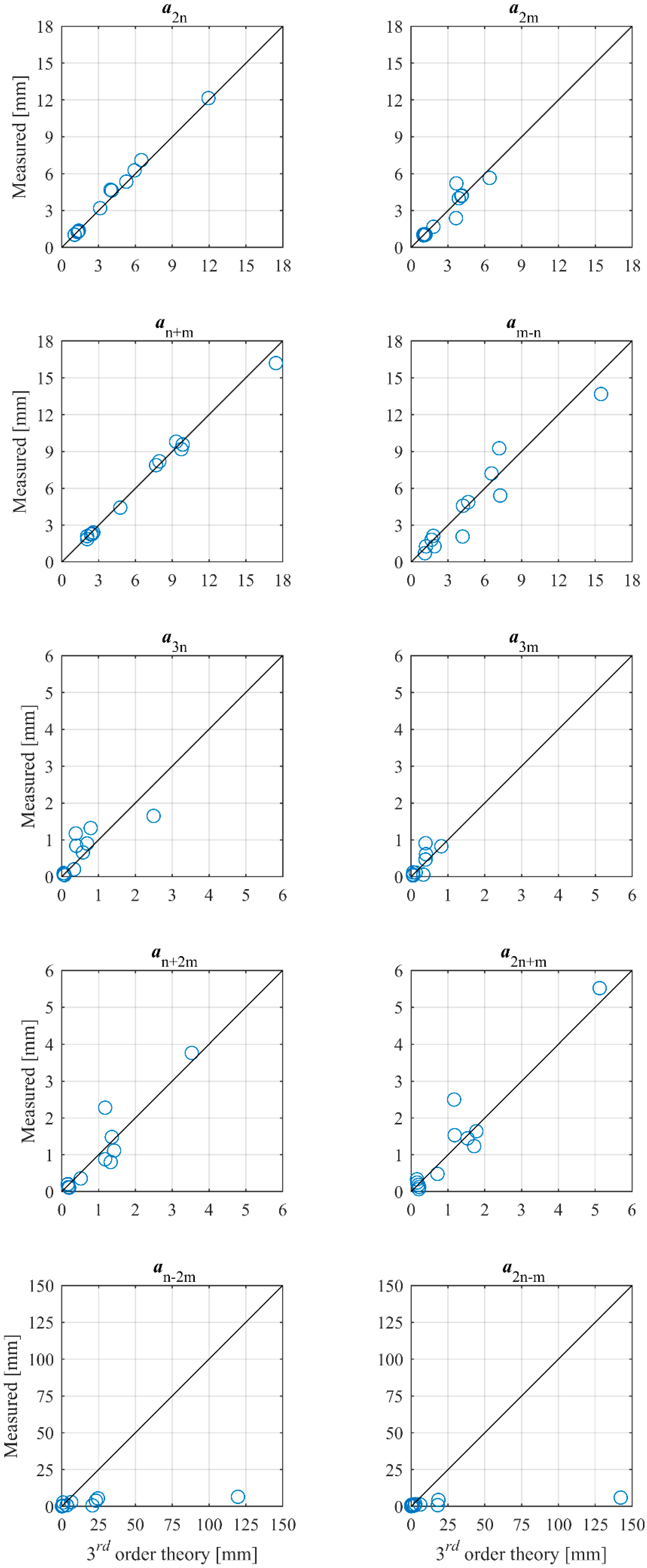
In Figure 6, the measured amplitudes from Table 3 are compared to theoretical predictions based on third-order wave theory (Madsen and Fuhrman [12,13]) using the two estimated primary amplitudes. The estimated amplitudes of the bound second-order superharmonics by the present method match accurately the ones predicted by the third-order theory. The same is the case for the subharmonic component, but more scatter is observed.
With respect to the third-order components, the agreement with third-order wave theory is fair except for the subharmonics, which presented strong deviations. The predicted amplitudes are significantly larger than the second-order components, which is not physically correct and is due to singularities in the transfer functions, as also found by Madsen and Fuhrman [13].
7. Discussion
In the present paper, a new method to separate nonlinear bichromatic waves into incident and reflected surface elevation time series was presented. Most existing methods only consider free energy to be present, and their range of applicability is thus limited to linear waves. The new method includes both free and bound higher harmonics, which is necessary in order to separate nonlinear waves accurately. The method is an extension of the method for nonlinear regular waves presented recently by Lykke Andersen et al. [7]. That method was extended by Eldrup and Lykke Andersen [8] to fully irregular waves by utilizing a narrow band approximation for the primary spectrum. The new method for bichromatic waves includes all interactions correctly to the third order. As expected, the results showed that the new method accurately predicted the incident and reflected waves in synthetically generated third-order bichromatic waves.
Moreover, the method was tested on physical model tests performed in a wave flume with wave makers in both ends. The new method seems to predict accurately the incident and reflected wave trains, and the estimated amplitudes of the second- and third-order bound components matched reasonably with third-order wave theory for irregular waves. For third-order subharmonics, a significant deviation from third-order wave theory was, however, found in some tests, but this could be attributed to singularities in the transfer functions provided by Madsen and Fuhrman [12,13], and thus their method was not valid for these cases.
Author Contributions
T.L.A. and M.R.E. defined the new analysis method, and M.R.E. prepared the synthetic and numerical model data. M.C. provided access to the wave flume and prepared the test setup for the physical model tests. T.L.A. prepared the test methodology and performed the model tests and the analysis. T.L.A. wrote the paper. All authors have read and approved the final manuscript.
Funding
This research received no external funding.
Conflicts of Interest
The authors declare no conflict of interest.
References
Goda, Y.; Suzuki, Y. Estimation of incident and reflected waves in random wave experiments. In Proceedings of the 15th International Conference on Coastal Engineering, Honolulu, HI, USA, 11–17 July 1976; pp. 828–845. [Google Scholar] [CrossRef]
Mansard, E.P.D.; Funke, E.R. The measurement of incident and reflected spectra using a least squares method. In Proceedings of the 17th International Conference on Coastal Engineering, Sydney, Australia, 23–29 March 1980; pp. 154–172. [Google Scholar] [CrossRef]
Zelt, J.A.; Skjelbreia, J.E. Estimating incident and reflected wave fields using an arbitrary number of wave gauges. In Proceedings of the 23rd International Conference on Coastal Engineering, Venice, Italy, 4–9 October 1992; pp. 777–788. [Google Scholar] [CrossRef]
Lin, C.-Y.; Huang, C.-J. Decomposition of incident and reflected higher harmonic waves using four wave gauges. Coast. Eng.2004, 51, 395–406. [Google Scholar] [CrossRef]
Figueres, M.; Garrido, J.M.; Medina, J.R. Cristalización Simulada para el Análisis de Oleaje Incidente y Reflejado con un Modelo de Onda Stokes-V; VII Jornadas de Puertos y Costas: Almeria, Spain, 2003. [Google Scholar]
Figueres, M.; Medina, J.R. Estimating incident and reflected waves using a fully nonlinear wave model. In Proceedings of the 29th International Conference on Coastal Engineering, Lisbon, Portugal, 19–24 September 2004; pp. 594–603. [Google Scholar] [CrossRef]
Lykke Andersen, T.; Eldrup, M.R.; Frigaard, P. Estimation of Incident and Reflected Components in Highly Nonlinear Regular Waves. Coast. Eng.2017, 119, 51–64. [Google Scholar] [CrossRef]
Eldrup, M.R.; Lykke Andersen, T. Estimation of Incident and Reflected Wave Trains in Highly Nonlinear Two-Dimensional Irregular Waves. J. Waterw. Port Coast. Ocean Eng.2019, 145. [Google Scholar] [CrossRef]
Fenton, J.D.; Rienecker, M.M. Accurate numerical solution for nonlinear waves. In Proceedings of the 17th Conference of Coastal Engineering, Sydney, Australia, 23–29 March 1980; Volume 1, pp. 50–69. [Google Scholar] [CrossRef]
Sharma, J.; Dean, R. Second-order directional seas and associated wave forces. Soc. Pet. Eng. J.1981, 21, 129–140. [Google Scholar] [CrossRef]
Schäffer, H.A. Laboratory Wave Generation Correct to Second Order. In Proceedings of the Conference Wave Kinematics and Environmental Forces, London, UK, 24–25 March 1993; Soc Underwater Tech. Volume 29, pp. 115–139. [Google Scholar]
Madsen, P.A.; Fuhrman, D.R. Third-order theory for bicromatic bi-directional water waves. J. Fluid Mech.2006, 557, 369–397. [Google Scholar] [CrossRef]
Madsen, P.A.; Fuhrman, D.R. Third-order theory for multi-directional irregular waves. J. Fluid Mech.2012, 698, 304–334. [Google Scholar] [CrossRef]
Lykke Andersen, T.; Clavero, M.; Frigaard, P.; Losada, M.; Puyol, J.I. A new active absorption system and its performance to linear and non-linear waves. Coast. Eng.2016, 114, 47–60. [Google Scholar] [CrossRef]
Le Mehauté, B. An Introduction to Hydrodynamics and Water Waves; Springer: Berlin/Heidelberg, Germany, 1976. [Google Scholar] [CrossRef]
Lykke Andersen, T.; Clavero, M.; Eldrup, M.R.; Frigaard, P.; Losada, M. Active Absorption of Nonlinear Irregular Wave. In Proceedings of the 36th International Conference on Coastal Engineering, Baltimore, MD, USA, 30 July–3 August 2018. submitted. [Google Scholar]
Figure 1.
Comparison of measured total and predicted incident and reflected time series at WG1 for the synthetic test case.
Figure 1.
Comparison of measured total and predicted incident and reflected time series at WG1 for the synthetic test case.
Figure 2.
Model test setup.
Figure 2.
Model test setup.
Figure 3.
Applicability of different wave theories for the test conditions.
Figure 3.
Applicability of different wave theories for the test conditions.
Figure 4.
Comparison of measured total and predicted incident and reflected time series at WG1 (x = 5.95 m) for Test No. 2.
Figure 4.
Comparison of measured total and predicted incident and reflected time series at WG1 (x = 5.95 m) for Test No. 2.
Figure 5.
Comparison of measured total and predicted incident and reflected time series at WG1 (x = 5.95 m) for Test No. 5.
Figure 5.
Comparison of measured total and predicted incident and reflected time series at WG1 (x = 5.95 m) for Test No. 5.
Figure 6.
Measured amplitudes of bound second- and third-order components compared to Madsen and Fuhrman [12,13].
Figure 6.
Measured amplitudes of bound second- and third-order components compared to Madsen and Fuhrman [12,13].
Table 1.
Actual and calculated amplitudes in millimeters for the synthetic test case.
Table 1.
Actual and calculated amplitudes in millimeters for the synthetic test case.
Component
Actual Incident Bound
Estimated Incident Bound
Estimated Reflected Bound
Estimated Incident Free
Estimated Reflected Free
an
50.0
50.1
0.2
-
-
am
50.0
49.9
0.2
-
-
a2n
5.8
5.8
0.0
0.0
0.0
a2m
4.7
4.7
0.0
0.1
0.1
an+m
10.5
10.5
0.0
0.2
0.1
am−n
7.4
7.6
0.1
0.3
0.1
a3n
0.7
0.7
0.0
0.0
0.0
a3m
0.5
0.5
0.0
0.0
0.0
an+2m
1.6
1.6
0.0
0.0
0.0
a2n+m
1.8
1.8
0.0
0.0
0.0
an−2m
7.7
7.7
0.0
0.0
0.0
am−2n
3.4
3.2
0.0
0.2
0.0
Table 2.
Target test conditions.
Table 2.
Target test conditions.
Test No.
fn [Hz]
fm [Hz]
an [mm]
am [mm]
1
0.30
0.40
50
50
2
0.50
0.60
50
50
3
0.60
0.70
50
50
4
0.60
0.80
50
50
5
0.50
0.55
50
50
6
0.50
0.52
50
50
7
0.30
0.40
25
25
8
0.50
0.60
25
25
9
0.60
0.70
25
25
10
0.60
0.80
25
25
11
0.50
0.55
25
25
12
0.50
0.52
25
25
Table 3.
Estimated amplitudes in millimeters of all the incident bound components.
Table 3.
Estimated amplitudes in millimeters of all the incident bound components.
Lykke Andersen, T.; Eldrup, M.R.; Clavero, M.
Separation of Long-Crested Nonlinear Bichromatic Waves into Incident and Reflected Components. J. Mar. Sci. Eng.2019, 7, 39.
https://doi.org/10.3390/jmse7020039
AMA Style
Lykke Andersen T, Eldrup MR, Clavero M.
Separation of Long-Crested Nonlinear Bichromatic Waves into Incident and Reflected Components. Journal of Marine Science and Engineering. 2019; 7(2):39.
https://doi.org/10.3390/jmse7020039
Chicago/Turabian Style
Lykke Andersen, Thomas, Mads R. Eldrup, and Maria Clavero.
2019. "Separation of Long-Crested Nonlinear Bichromatic Waves into Incident and Reflected Components" Journal of Marine Science and Engineering 7, no. 2: 39.
https://doi.org/10.3390/jmse7020039
APA Style
Lykke Andersen, T., Eldrup, M. R., & Clavero, M.
(2019). Separation of Long-Crested Nonlinear Bichromatic Waves into Incident and Reflected Components. Journal of Marine Science and Engineering, 7(2), 39.
https://doi.org/10.3390/jmse7020039
Note that from the first issue of 2016, this journal uses article numbers instead of page numbers. See further details here.
Article Metrics
No
No
Article Access Statistics
For more information on the journal statistics, click here.
Multiple requests from the same IP address are counted as one view.
Lykke Andersen, T.; Eldrup, M.R.; Clavero, M.
Separation of Long-Crested Nonlinear Bichromatic Waves into Incident and Reflected Components. J. Mar. Sci. Eng.2019, 7, 39.
https://doi.org/10.3390/jmse7020039
AMA Style
Lykke Andersen T, Eldrup MR, Clavero M.
Separation of Long-Crested Nonlinear Bichromatic Waves into Incident and Reflected Components. Journal of Marine Science and Engineering. 2019; 7(2):39.
https://doi.org/10.3390/jmse7020039
Chicago/Turabian Style
Lykke Andersen, Thomas, Mads R. Eldrup, and Maria Clavero.
2019. "Separation of Long-Crested Nonlinear Bichromatic Waves into Incident and Reflected Components" Journal of Marine Science and Engineering 7, no. 2: 39.
https://doi.org/10.3390/jmse7020039
APA Style
Lykke Andersen, T., Eldrup, M. R., & Clavero, M.
(2019). Separation of Long-Crested Nonlinear Bichromatic Waves into Incident and Reflected Components. Journal of Marine Science and Engineering, 7(2), 39.
https://doi.org/10.3390/jmse7020039
Note that from the first issue of 2016, this journal uses article numbers instead of page numbers. See further details here.


