2D Numerical Study of the Stability of Trench under Wave Action in the Immersing Process of Tunnel Element

Abstract
1. Introduction
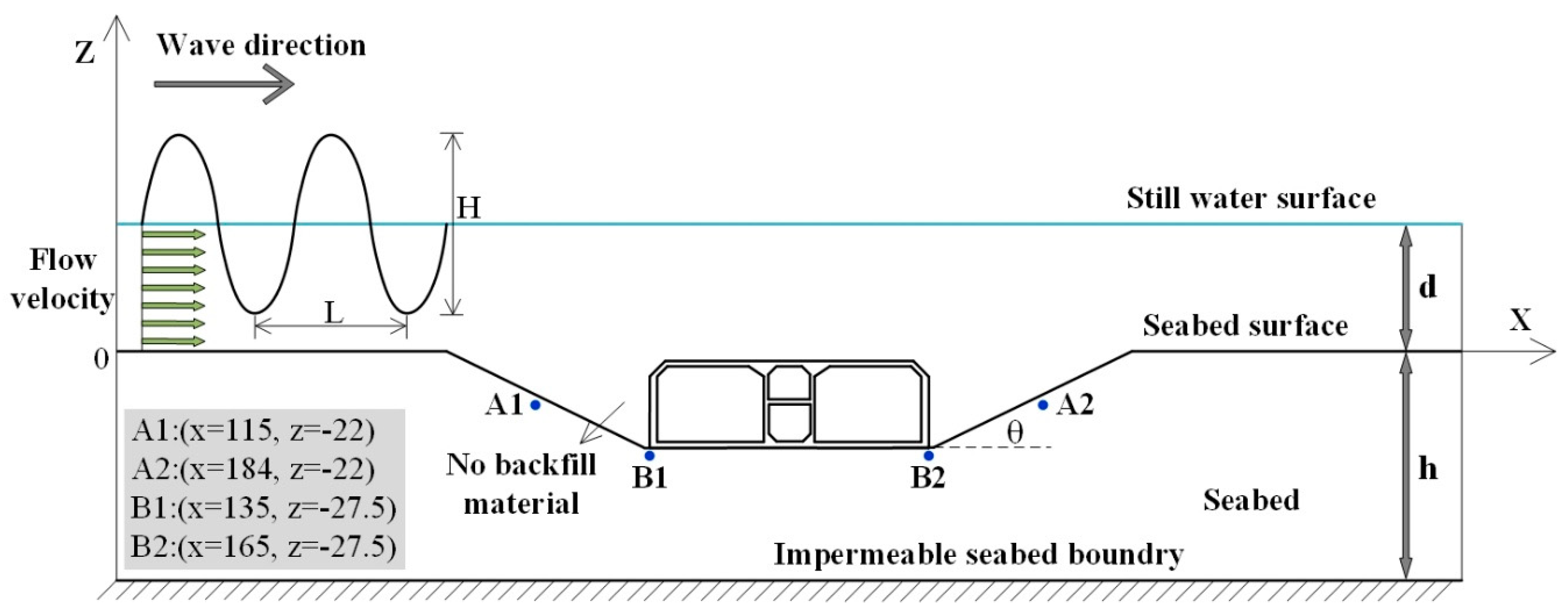
2. Numerical Model
2.1. Fluid Dynamic Model
2.2. Seabed Model
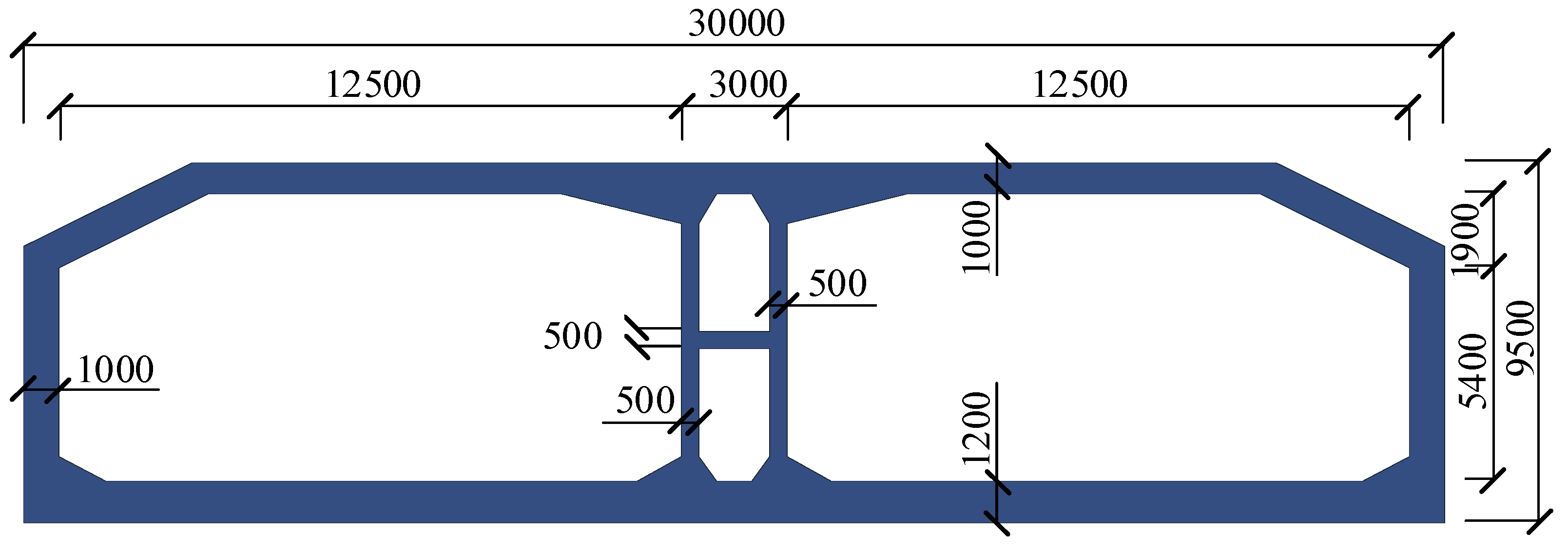
2.3. Tunnel Model
2.4. Boundary Conditions
2.4.1. Seabed Boundary Conditions
2.4.2. Tunnel Boundary Conditions
2.4.3. Free Water Surface Boundary Conditions
2.5. Integration of Fluid Dynamic Model and Seabed Model
3. Model Validation and Numerical Results
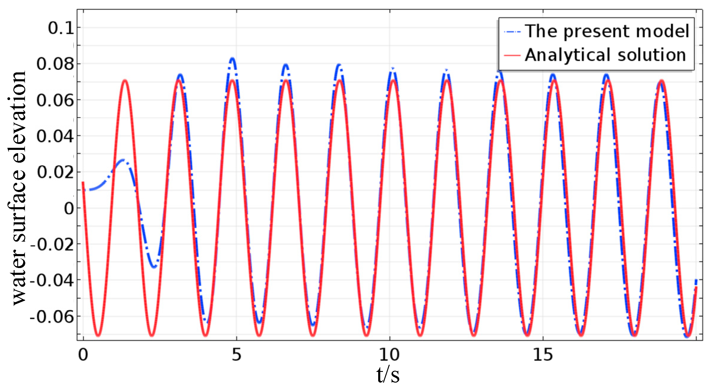
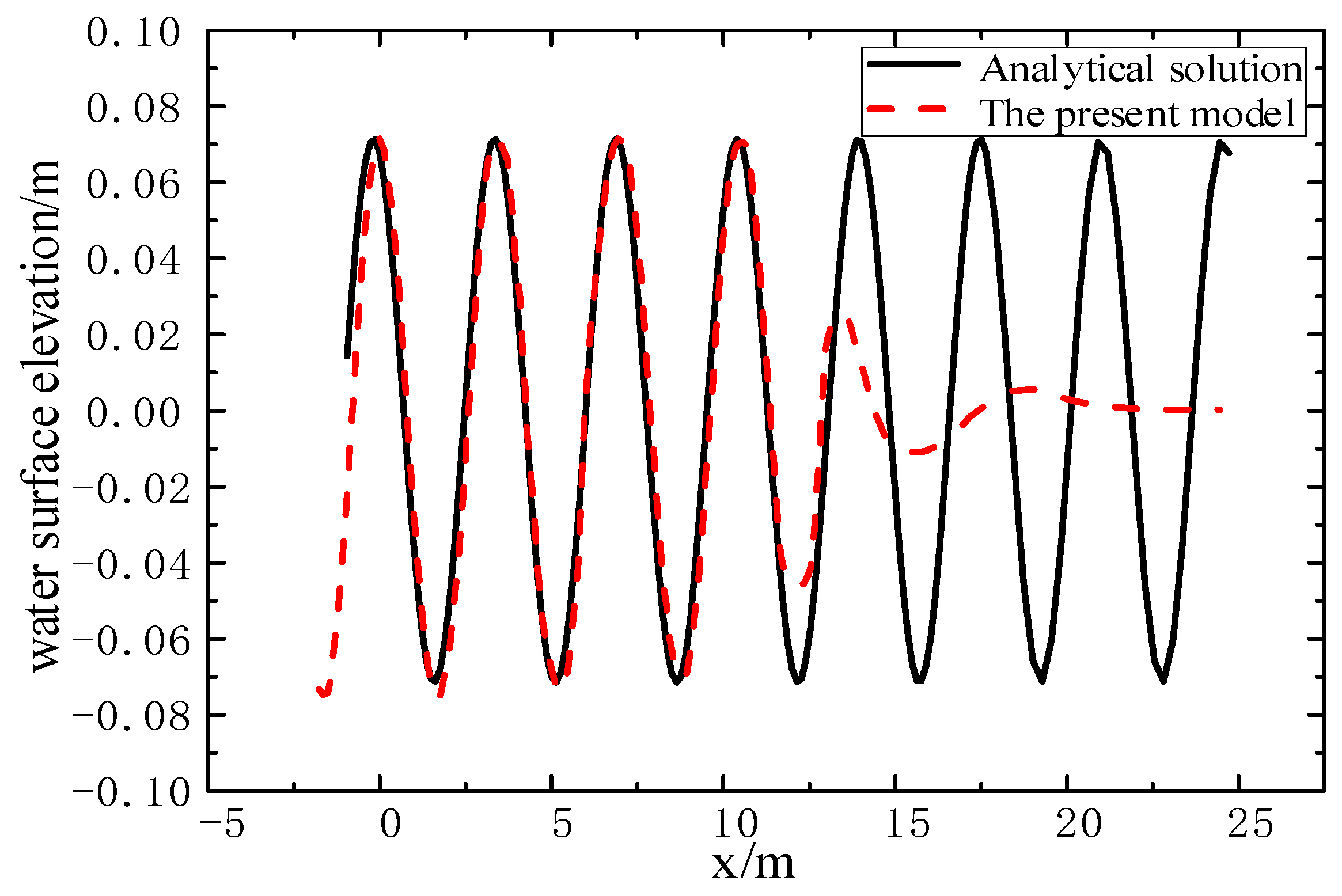
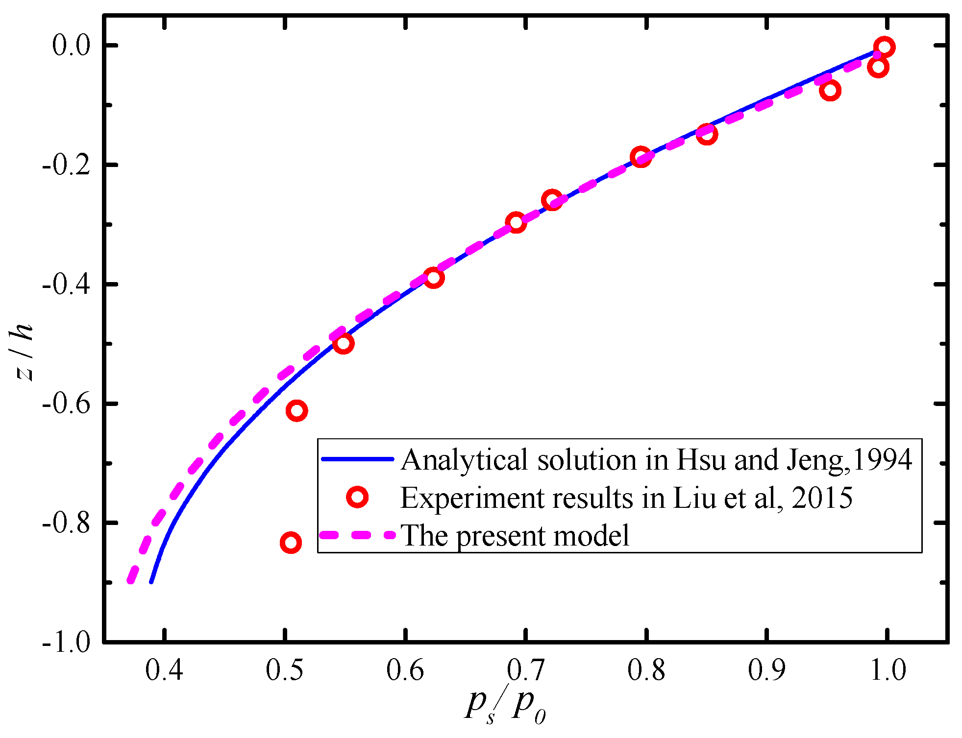
3.1. Model Validation
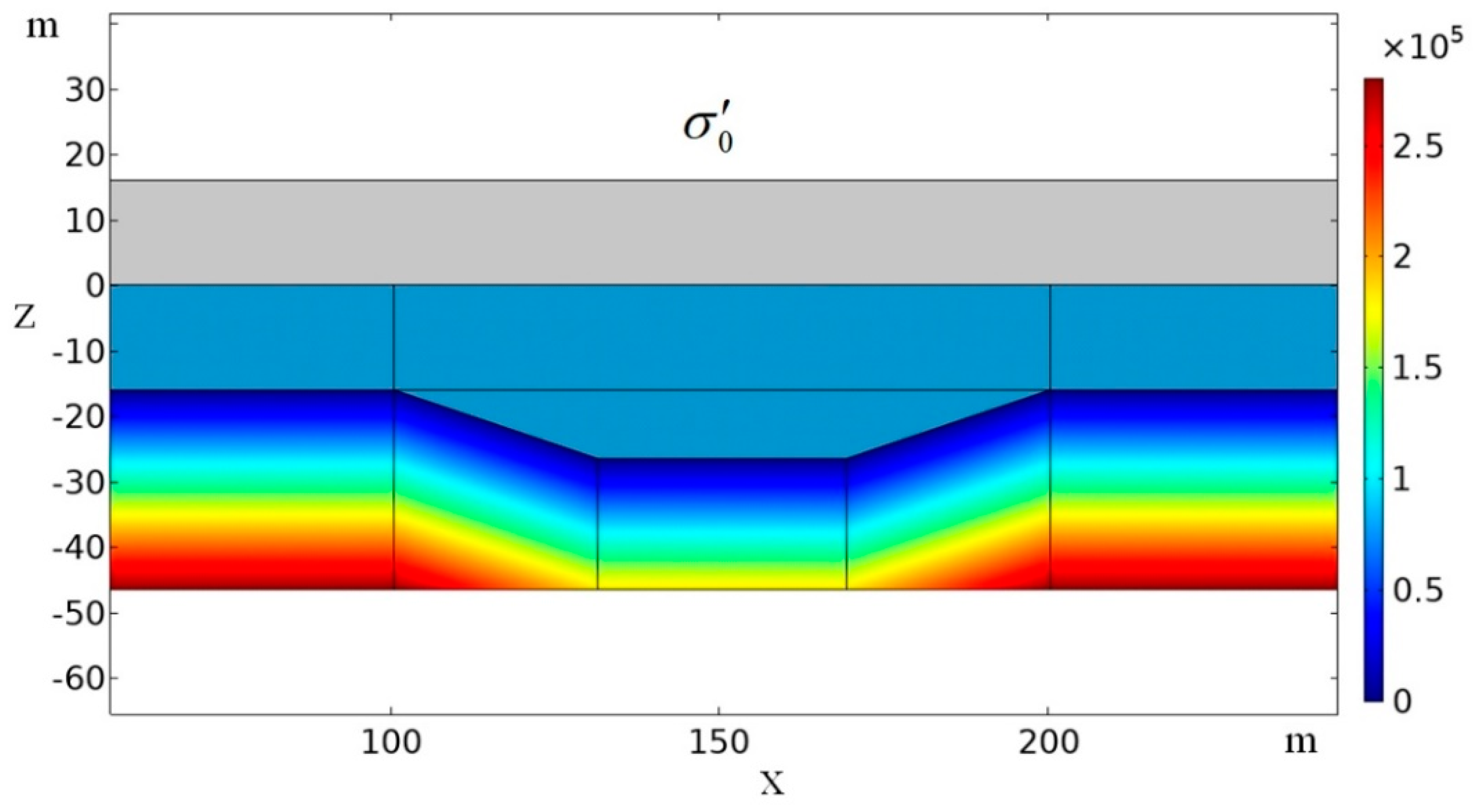
3.2. Consolidation of the Seabed
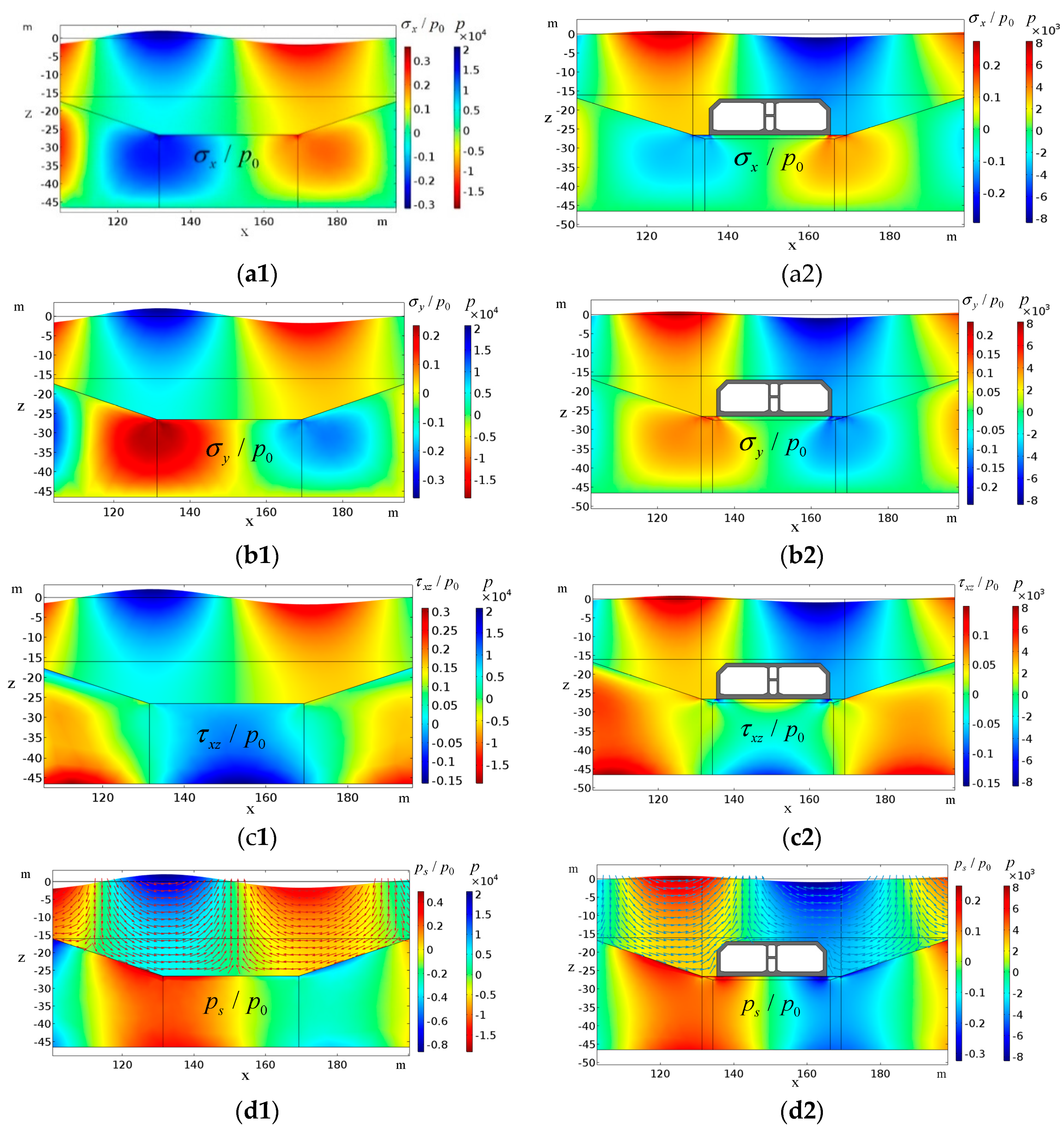
3.3. Dynamic Responses of the Seabed
3.4. Wave-Induced Liquefaction
3.5. Wave-Induced Shear Failure
3.6. Influence of Wave Characters on Liquefaction
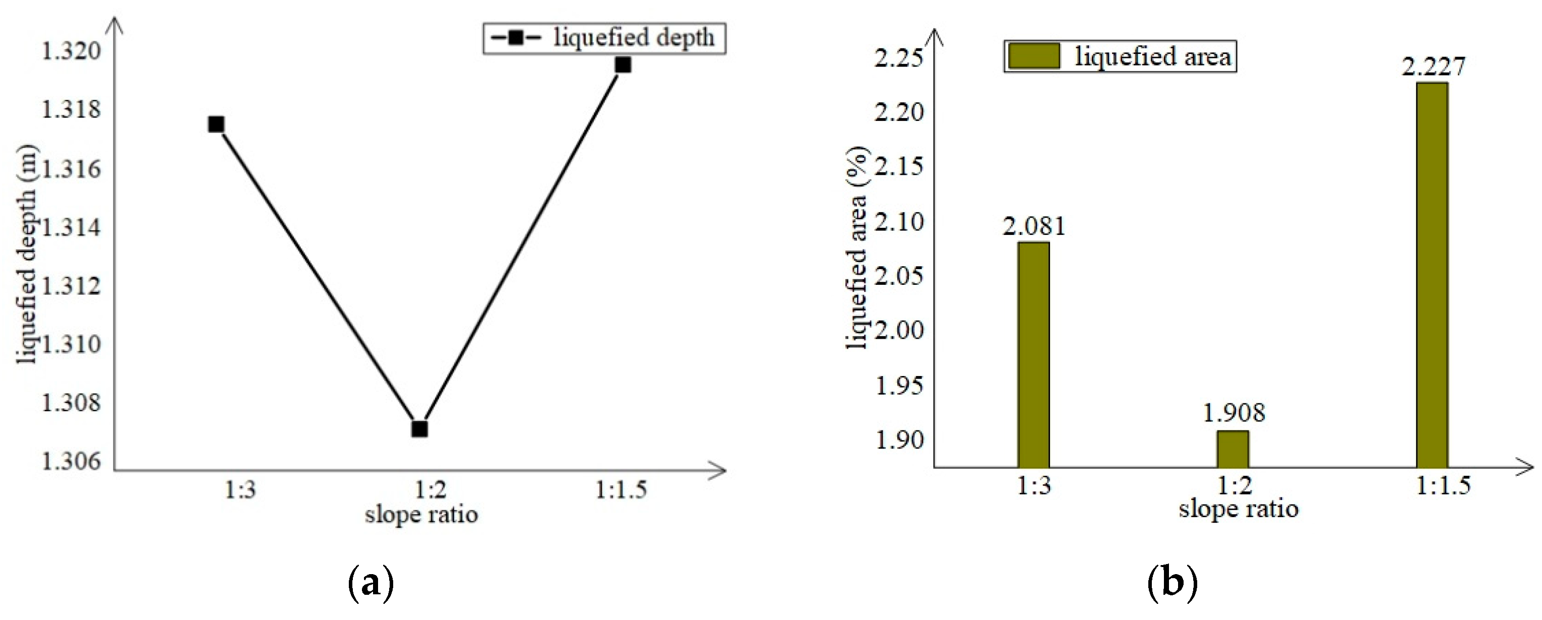
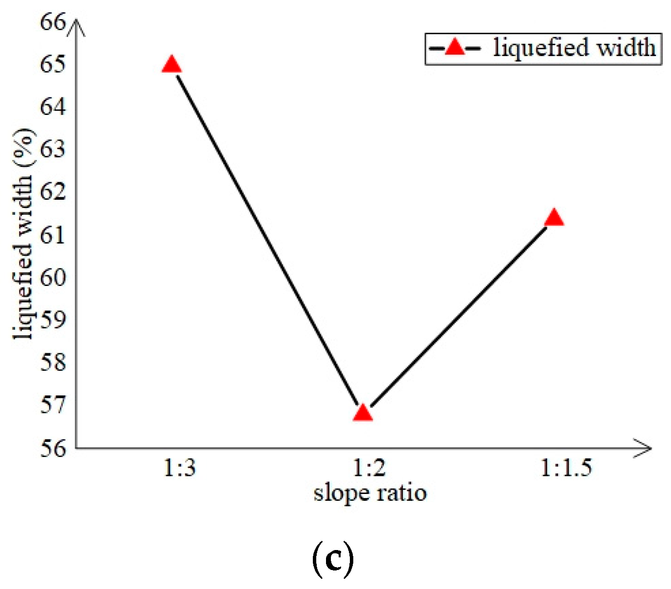
3.7. Influence of Slope Rate on Liquefaction
4. Conclusions
- (1)
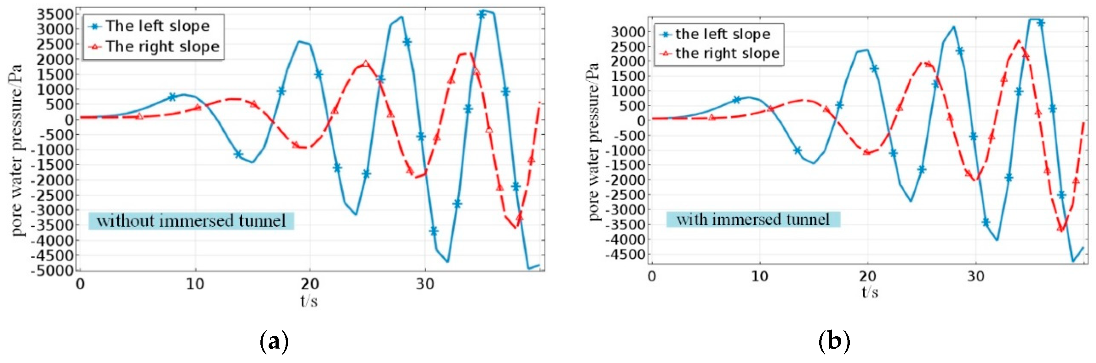
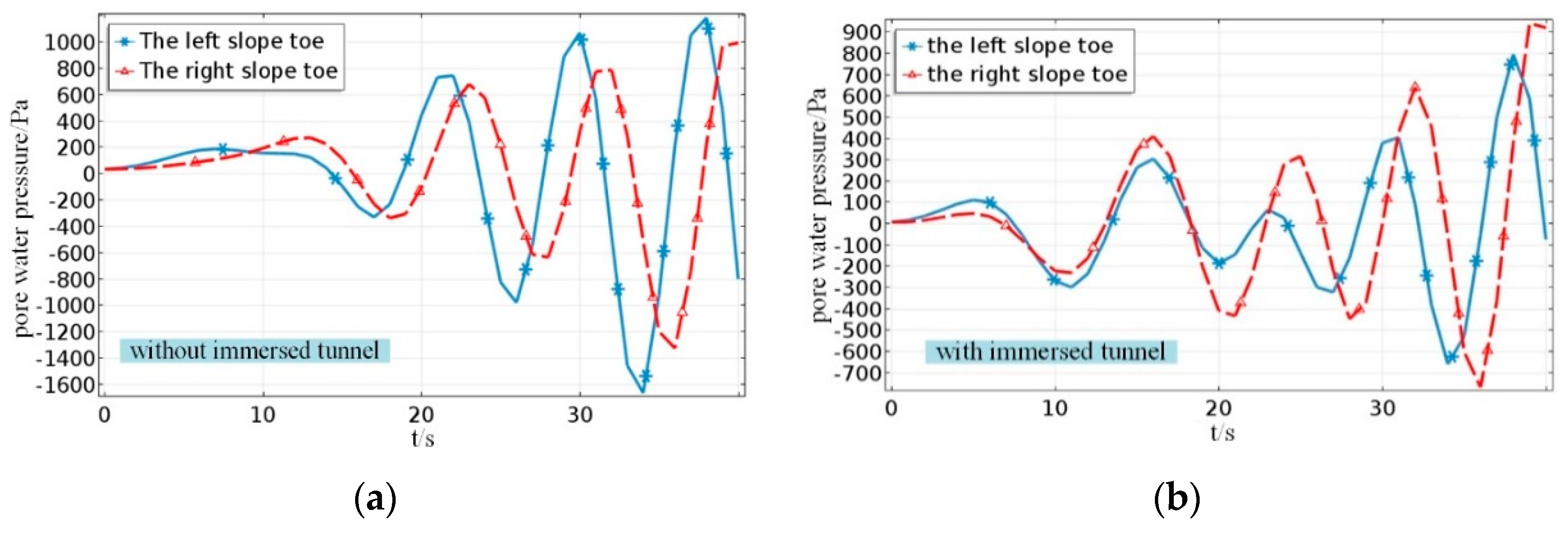
- Due to the existence of the trench, the pore pressure amplitude on the weather side slope is significantly smaller than that on the lee side slope.
- (2)
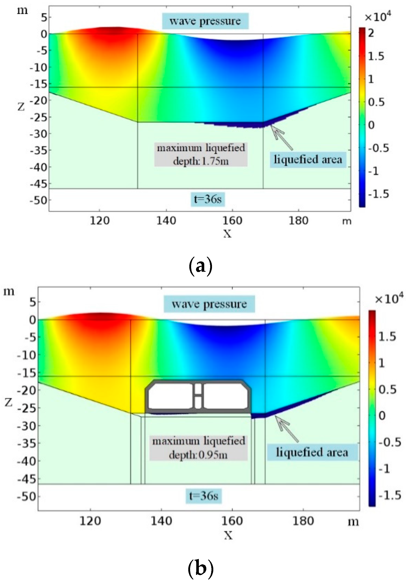
- The maximum depth of liquefaction in the case after the tunnel element is placed is smaller than that after the foundation groove is excavated.
- (3)
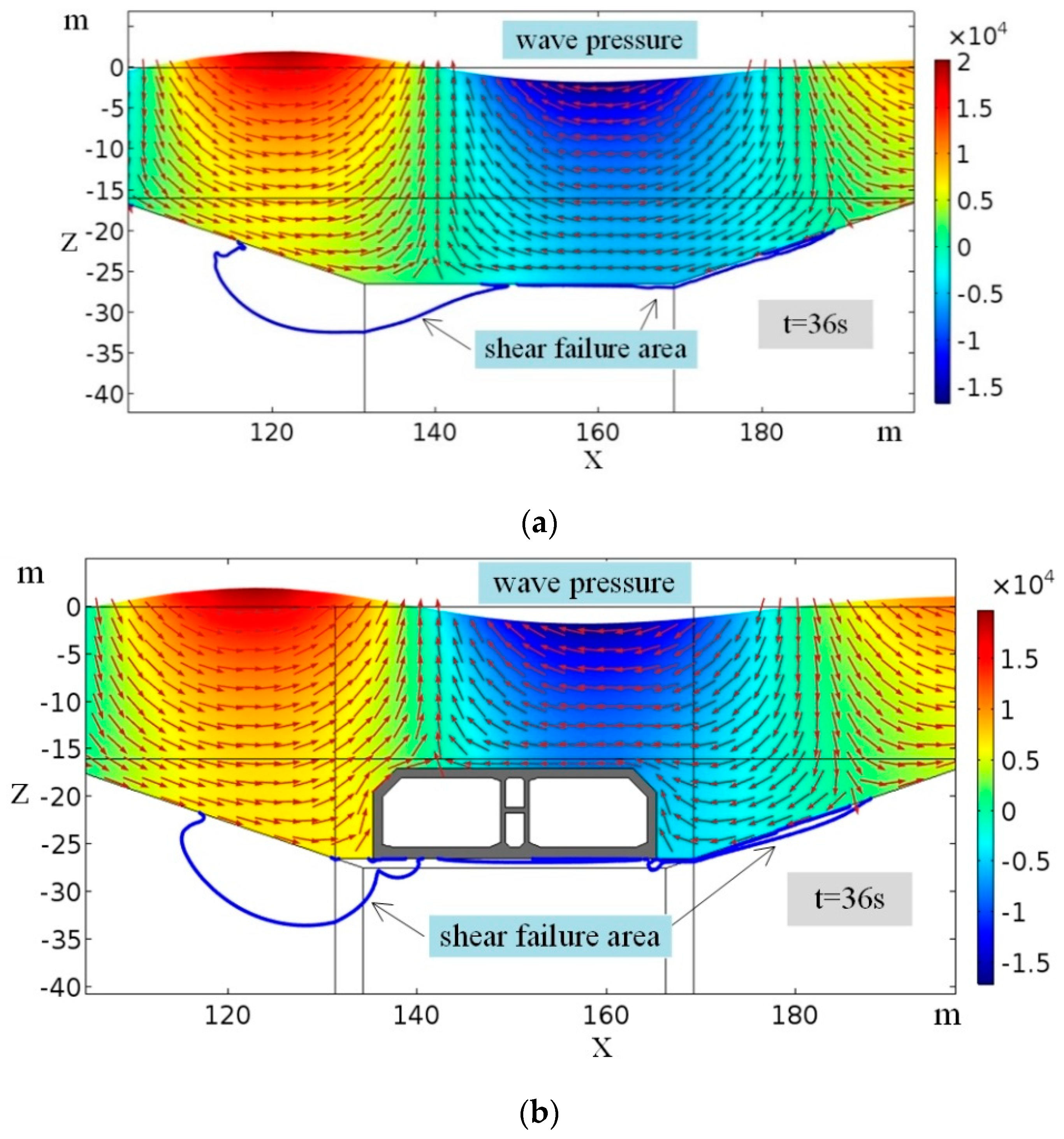
- Due to the existence of the tunnel structure, the distribution of the flow field and pressure field change dramatically; thus, the dynamic responses and the failure area in the seabed change accordingly.
- (4)
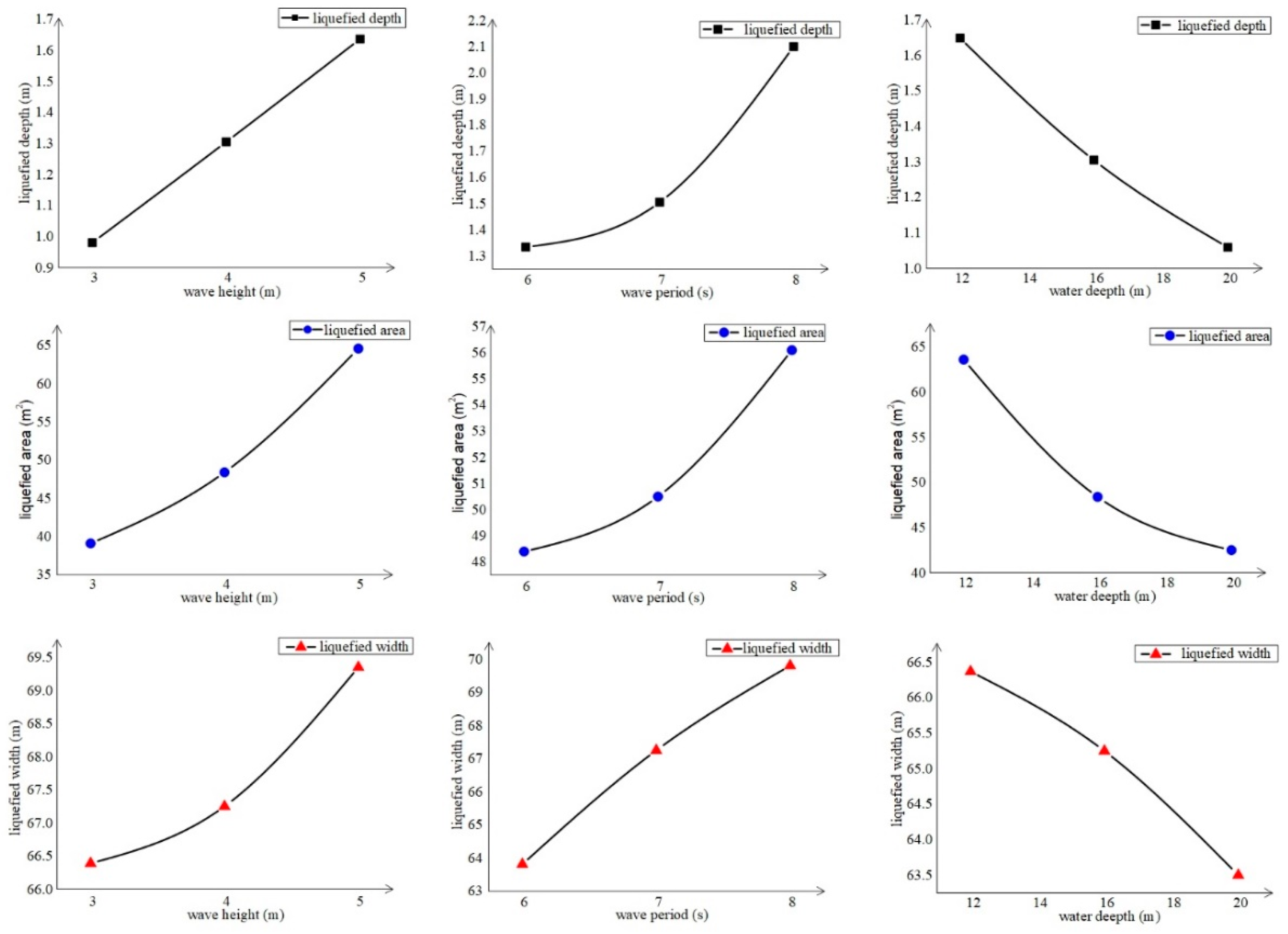
- In the case of the specific wave and seabed parameters, the liquefaction characteristics in the trench have an obvious fold point with the change of slope rate. That means that there is an optimal slope rate to minimize the failure possibility of the slope. Moreover, the specific failure mode deserves further research.
Author Contributions
Funding
Acknowledgments
Conflicts of Interest
References
- Yamamoto, T.; Koning, H.L.; Sellmeijer, H.; Hijum, E.V. On the response of a poroelastic bed to water waves. J. Fluid Mech. 1978, 87, 193–206. [Google Scholar] [CrossRef]
- Okusa, S. Wave-induced stress in unsaturated submarine sediments. Géotechnique 1985, 35, 517–532. [Google Scholar] [CrossRef]
- Ye, J.H.; Jeng, D.S. Effects of bottom shear stresses on the wave-induced dynamic response in a porous seabed: PORO-WSSI (shear) model. Acta Mech. 2011, 27, 898–910. [Google Scholar] [CrossRef]
- Zhang, C.; Zhang, Q.Y.; Zheng, J.H.; Demirbilek, Z. Parameterization of nearshore wave front slope. Coast. Eng. 2017, 127, 80–87. [Google Scholar] [CrossRef]
- Zheng, J.H.; Zhang, C.; Demirbilek, Z.; Lin, L.W. Numerical study of sandbar migration under wave-undertow interaction. J. Waterw. Port Coast. Ocean Eng. 2014, 140, 146–159. [Google Scholar] [CrossRef]
- Jeng, D.S.; Ye, J.H.; Zhang, J.S.; Liu, P.L.F. An integrated model for the wave induced seabed response around marine structures: Model verifications and applications. Coast. Eng. 2013, 72, 1–19. [Google Scholar] [CrossRef]
- Sumer, B.M. Liquefaction around Marine Structures; Liu, P.L.F., Ed.; World Scientific: Singapore, 2014. [Google Scholar]
- Guo, Z.; Jeng, D.S.; Zhao, H.Y.; Guo, W.; Wang, L.Z. Effect of Seepage Flow on Sediment Incipient Motion around a Free Spanning Pipeline. Coast. Eng. 2019, 143, 50–62. [Google Scholar] [CrossRef]
- Li, K.; Guo, Z.; Wang, L.Z.; Jiang, H.Y. Effect of Seepage Flow on Shields Number around a Fixed and Sagging Pipeline. Ocean Eng. 2019, 172, 487–500. [Google Scholar] [CrossRef]
- Qi, W.G.; Li, Y.X.; Xu, K.; Gao, F.P. Physical modelling of local scour at twin piles under combined waves and current. Coast. Eng. 2019, 143, 63–75. [Google Scholar] [CrossRef]
- He, R.; Kaynia, A.M.; Zhang, J.S.; Chen, W.Y.; Guo, Z. Influence of vertical shear stresses due to pile-soil interaction on lateral dynamic responses for offshore monopoles. Mar. Struct. 2019, 64, 341–359. [Google Scholar] [CrossRef]
- Chen, W.Y.; Chen, G.X.; Chen, W.; Liao, C.C.; Gao, H.M. Numerical simulation of the nonlinear wave-induced dynamic response of anisotropic poro-elastoplastic seabed. Mar. Georesour. Geotechnol. 2018, 1–12. [Google Scholar] [CrossRef]
- Chen, W.Y.; Fang, D.; Chen, G.X.; Jeng, D.S.; Zhu, J.F.; Zhao, H.Y. A simplified quasi-static analysis of wave-induced residual liquefaction of seabed around an immersed tunnel. Ocean Eng. 2018, 148, 574–587. [Google Scholar] [CrossRef]
- Sui, T.; Zheng, J.; Zhang, C.; Jeng, D.S.; Zhang, J.; Guo, Y.; He, R. Consolidation of unsaturated seabed around an inserted pile foundation and its effects on the wave-induced momentary liquefaction. Ocean Eng. 2017, 131, 308–321. [Google Scholar] [CrossRef]
- Sui, T.; Zhang, C.; Guo, Y.; Zheng, J.; Jeng, D.; Zhang, J.; Zhang, W. Three-dimensional numerical model for wave-induced seabed response around mono-pile. Ships Offshore Struc. 2016, 11, 667–678. [Google Scholar] [CrossRef]
- Qi, W.G.; Gao, F.P. Wave induced instantaneously-liquefied soil depth in a non-cohesive seabed. Ocean Eng. 2018, 153, 412–423. [Google Scholar] [CrossRef]
- Jeng, D.S.; Rahman, M. Effective stresses in a porous seabed of finite thickness: Inertia effects. Can. Geotech. J. 2000, 37, 1383–1392. [Google Scholar] [CrossRef]
- Liao, C.C.; Jeng, D.S.; Zhang, L.L. An analytical approximation for dynamic soil response of a porous seabed due to combined wave and current loading. J. Coast. Res. 2013, 31, 1120–1128. [Google Scholar] [CrossRef]
- Yuhi, M.; Ishida, H. Analytical solution for wave-induced seabed response in a soil-water two-phase mixture. Coast. Eng. J. 2014, 40, 367–381. [Google Scholar] [CrossRef]
- Jeng, D.S.; Cheng, L. Wave-induced seabed instability around a buried pipeline in a poro-elastic seabed. Ocean Eng. 2000, 27, 127–146. [Google Scholar] [CrossRef]
- Zhao, H.Y.; Liang, Z.D.; Jeng, D.S.; Zhu, J.F.; Guo, Z.; Chen, W.Y. Numerical investigation of dynamic soil response around a submerged rubble mound breakwater. Ocean Eng. 2018, 156, 406–423. [Google Scholar] [CrossRef]
- Kasper, T.; Steenfelt, J.S.; Pedersen, L.M.; Jackson, P.G.; Heijmans, R.W.M.G. Stability of an immersed tunnel in offshore conditions under deep water wave impact. Coast. Eng. 2008, 55, 753–760. [Google Scholar] [CrossRef]
- Liao, C.; Tong, D.; Jeng, D.S.; Zhao, H.Y. Numerical study for wave-induced oscillatory pore pressures and liquefaction around impermeable slope breakwater heads. Ocean Eng. 2018, 157, 364–375. [Google Scholar] [CrossRef]
- Liao, C.; Tong, D.; Chen, L. Pore pressure distribution and momentary liquefaction in vicinity of impermeable slope-type breakwater head. Appl. Ocean Res. 2018, 78, 290–306. [Google Scholar] [CrossRef]
- Wei, G.; Kirby, J.T.; Sinha, A. Generation of waves in Boussinesq models using a source function method. Coast. Eng. 1999, 36, 271–299. [Google Scholar] [CrossRef]
- Choi, J.; Yoon, S.B. Numerical simulations using momentum source wave-maker applied to RANS equation model. Coast. Eng. 2009, 56, 1043–1060. [Google Scholar] [CrossRef]
- Launder, B.E.; Spalding, D.B. The numerical computation of turbulence flows. Comput. Methods Appl. Mech. Eng. 1974, 3, 269–289. [Google Scholar] [CrossRef]
- Rodi, W. Turbulence Models and Their Application in Hydraulics; Routledge: Abingdon, UK, 2017. [Google Scholar]
- Olsson, E.; Kreiss, G.; Zahedi, S. A conservative level set method for two phase flow II. J. Comput. Phys. 2007, 225, 785–807. [Google Scholar] [CrossRef]
- Desjardins, O.; Moureau, V.; Pitsch, H. An accurate conservative level set/ghost fluid method for simulating turbulent atomization. J. Comput. Phys. 2008, 227, 8395–8416. [Google Scholar] [CrossRef]
- Sheu, T.W.H.; Yu, C.H.; Chiu, P.H. Development of a dispersively accurate conservative level set scheme for capturing interface in two-phase flows. J. Comput. Phys. 2009, 228, 661–686. [Google Scholar] [CrossRef]
- Verruijt, A. Elastic Storage of Aquifers. In Flow through Porous Media; Academic Press: New York, NY, USA, 1969. [Google Scholar]
- Liu, B.; Jeng, D.S.; Ye, G.L. Laboratory study for pore pressures in sandy deposit under wave loading. Ocean Eng. 2015, 106, 207–219. [Google Scholar] [CrossRef]
- Hsu, J.R.C.; Jeng, D.S. Wave-induced soil response in an unsaturated anisotropic seabed of finite thickness. Int. J. Numer. Anal. Methods Geomech. 1994, 18, 785–807. [Google Scholar] [CrossRef]
- Zen, K.; Yamamoto, H. Oscillatory pore pressure and liquefaction in seabed induced by ocean waves. SOILS Found. 1990, 30, 161–179. [Google Scholar] [CrossRef]
- Sakai, T.; Hatanaka, K.; Mase, H. Wave-induced effective stress in seabed and its momentary liquefaction. J. Waterw. Port Coast. Ocean Eng. 1992, 118, 202–206. [Google Scholar] [CrossRef]
- Jeng, D.S.; Seymour, B.; Gao, F.P.; Wu, Y.X. Ocean waves propagating over a porous seabed: Residual and oscillatory mechanisms. Sci. China Ser. E 2007, 50, 81–89. [Google Scholar] [CrossRef]
- Jeng, D.S. Mechanism of the wave-induced seabed instability in the vicinity of a breakwater: A review. Ocean Eng. 2001, 2, 537–570. [Google Scholar] [CrossRef]
- Zen, K.; Jeng, D.S.; Hsu, J.R.C.; Ohyama, T. Wave-induced seabed instability: Difference between liquefaction and shear failure. Soils Found. 1998, 38, 37–47. [Google Scholar] [CrossRef]


| shear modulus () | 1.27 × 10⁷ N/m2 |
| poison’s ratio () | 0.3 |
| soil permeability () | 1.8 × 10⁻⁴ m/s |
| soil porosity () | 0.425 |
| saturation degree () | 0.995 |
| seabed thickness () | 1.8 m |
| Wave Parameters | Value | Unit |
|---|---|---|
| wave height () | 2 | m |
| wave period () | 8 | s |
| wave length () | 83.4 | m |
| water depth () | 16 | m |
| Soil Parameters | ||
| seabed thickness () | 30.5 | m |
| shear modulus () | 5 × 10⁶ | N/m2 |
| soil porosity () | 0.45 | - |
| poison’s ratio () | 0.27 | - |
| elastic modulus () | 3 × 10⁷ | N/m2 |
| soil permeability () | 10−6 | m/s |
| saturation degree () | 0.975 | - |
| density of soil grain () | 2650 | kg/m3 |
| internal cohesion () | 0 | kPa |
| internal friction angle () | 30 | deg |
| Water Parameters | ||
| shear modulus () | 2 × 10⁹ | N/m2 |
| density of water () | 986 | kg/m3 |
| Tunnel Parameters | ||
| elastic modulus () | 3.5 × 10¹⁰ | N/m2 |
| poison’s ratio () | 0.18 | - |
| density of tunnel () | 2700 | kg/m3 |
© 2019 by the authors. Licensee MDPI, Basel, Switzerland. This article is an open access article distributed under the terms and conditions of the Creative Commons Attribution (CC BY) license (http://creativecommons.org/licenses/by/4.0/).
Share and Cite
Chen, W.-Y.; Liu, C.-L.; Duan, L.-L.; Qiu, H.-M.; Wang, Z.-H. 2D Numerical Study of the Stability of Trench under Wave Action in the Immersing Process of Tunnel Element. J. Mar. Sci. Eng. 2019, 7, 57. https://doi.org/10.3390/jmse7030057
Chen W-Y, Liu C-L, Duan L-L, Qiu H-M, Wang Z-H. 2D Numerical Study of the Stability of Trench under Wave Action in the Immersing Process of Tunnel Element. Journal of Marine Science and Engineering. 2019; 7(3):57. https://doi.org/10.3390/jmse7030057
Chicago/Turabian StyleChen, Wei-Yun, Cheng-Lin Liu, Lun-Liang Duan, Hao-Miao Qiu, and Zhi-Hua Wang. 2019. "2D Numerical Study of the Stability of Trench under Wave Action in the Immersing Process of Tunnel Element" Journal of Marine Science and Engineering 7, no. 3: 57. https://doi.org/10.3390/jmse7030057
APA StyleChen, W.-Y., Liu, C.-L., Duan, L.-L., Qiu, H.-M., & Wang, Z.-H. (2019). 2D Numerical Study of the Stability of Trench under Wave Action in the Immersing Process of Tunnel Element. Journal of Marine Science and Engineering, 7(3), 57. https://doi.org/10.3390/jmse7030057