Study on the Spillover of Sediment during Typical Tidal Processes in the Yangtze Estuary Using a High-Resolution Numerical Model


Abstract
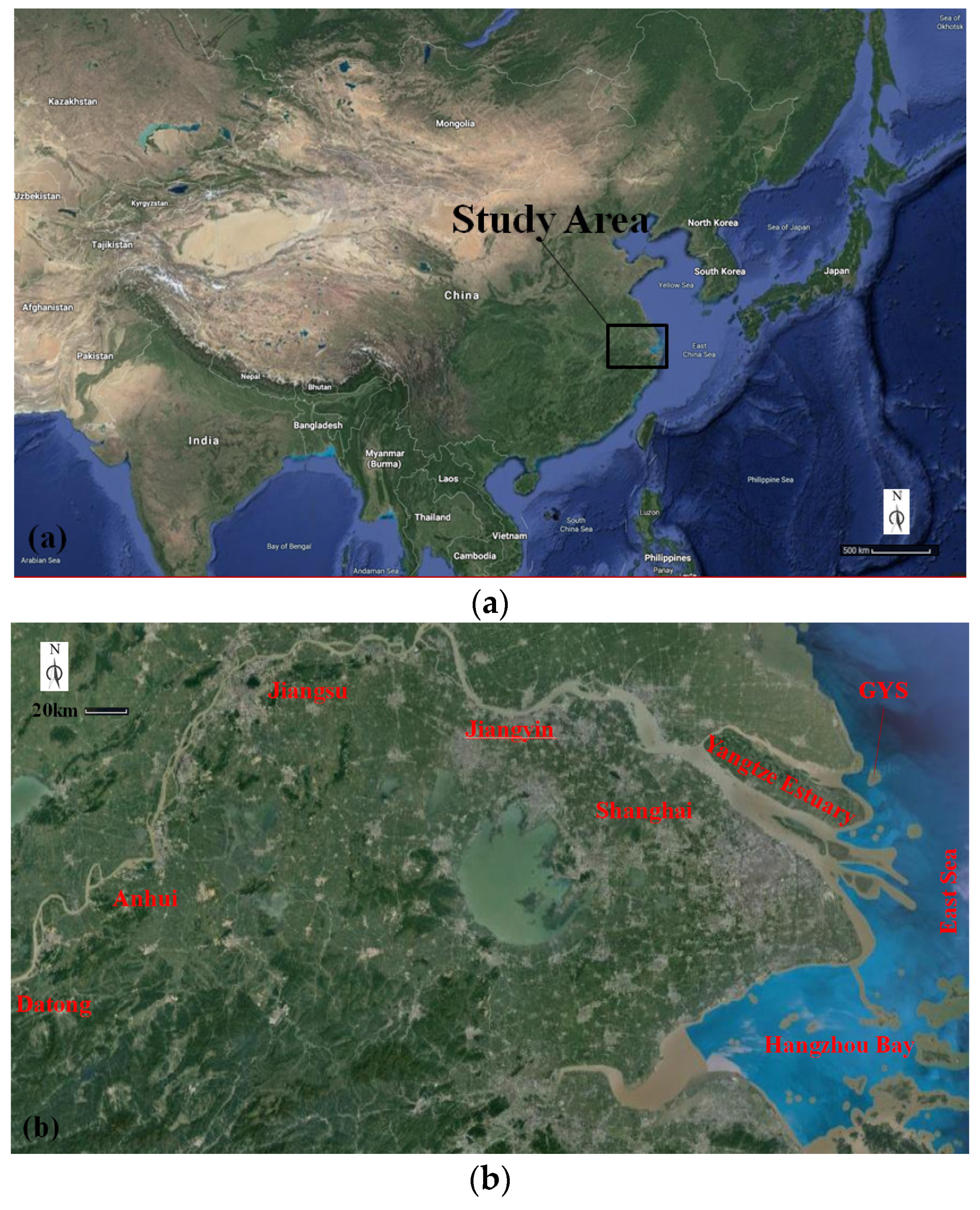
:1. Introduction
2. Numerical Formulation
2.1. Governing Equations
2.2. Computational Grid and Model Formulation
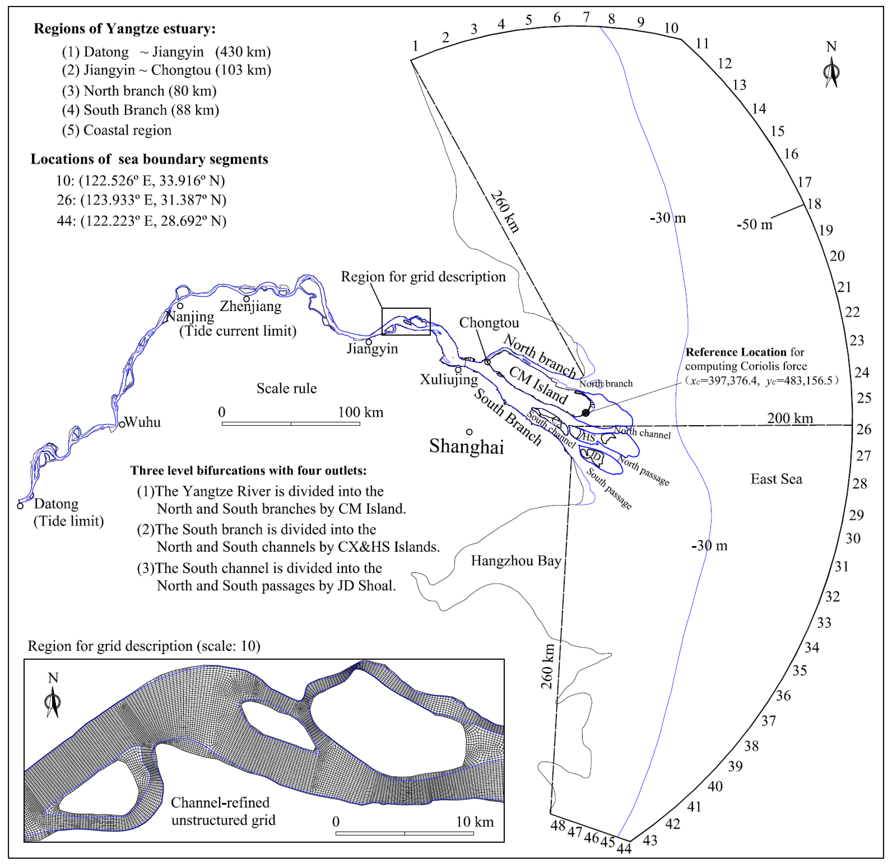
2.2.1. Computational Grid
2.2.2. Numerical Discretizations
2.3. Parallelization of the Model Code
3. Model Parameters and Tests
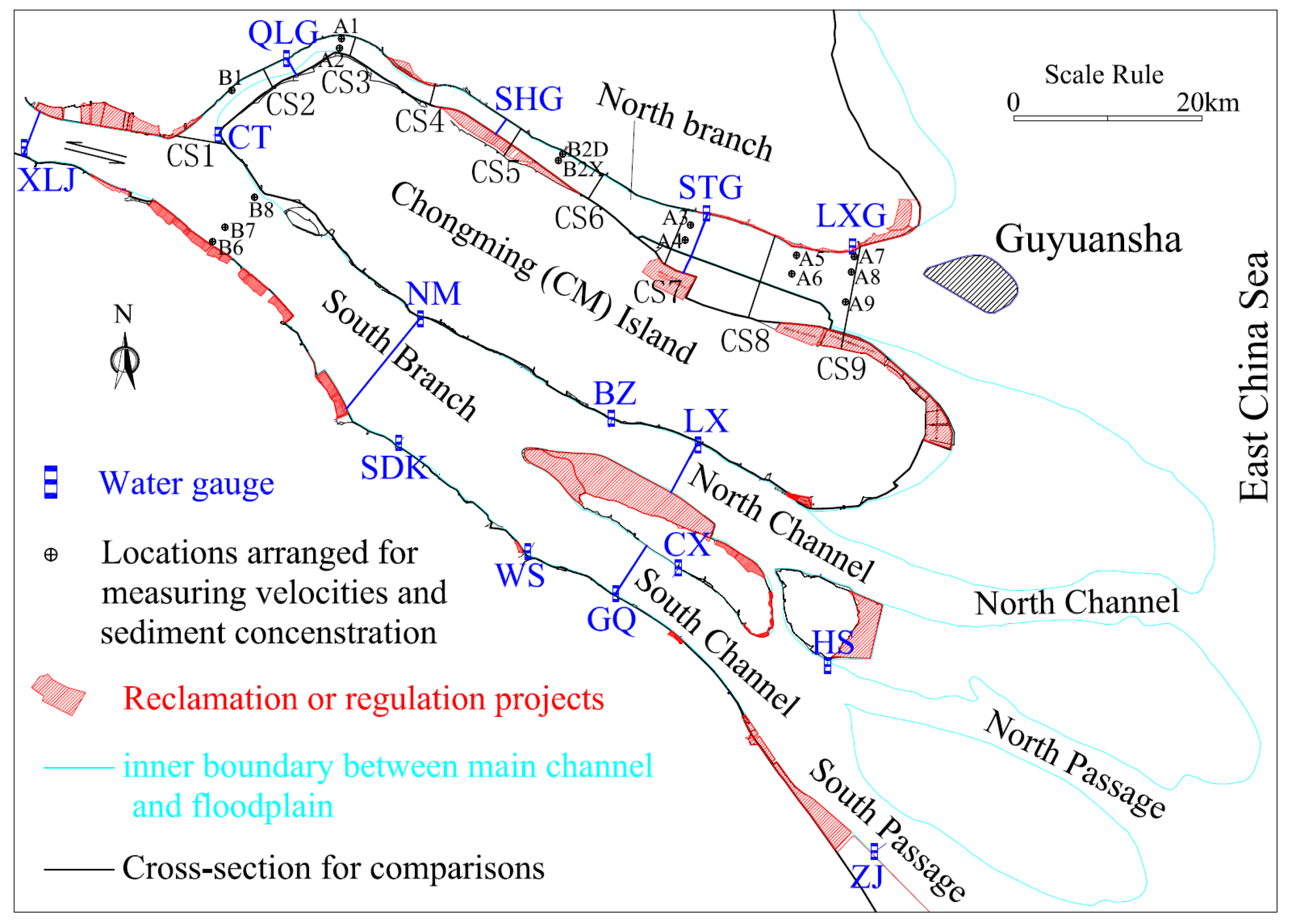
3.1. Computational Grid and Boundary Conditions
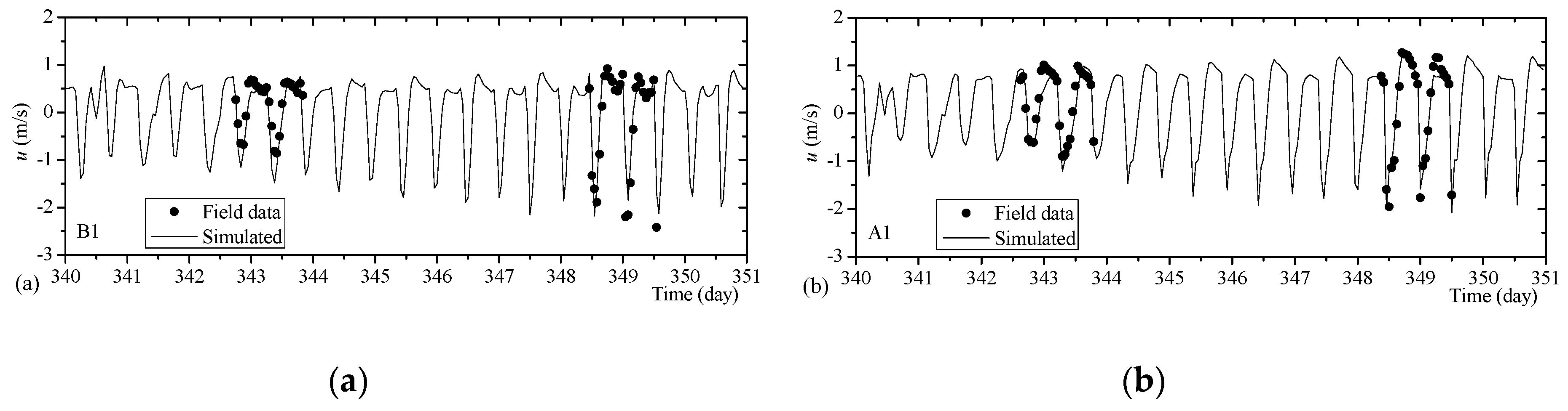
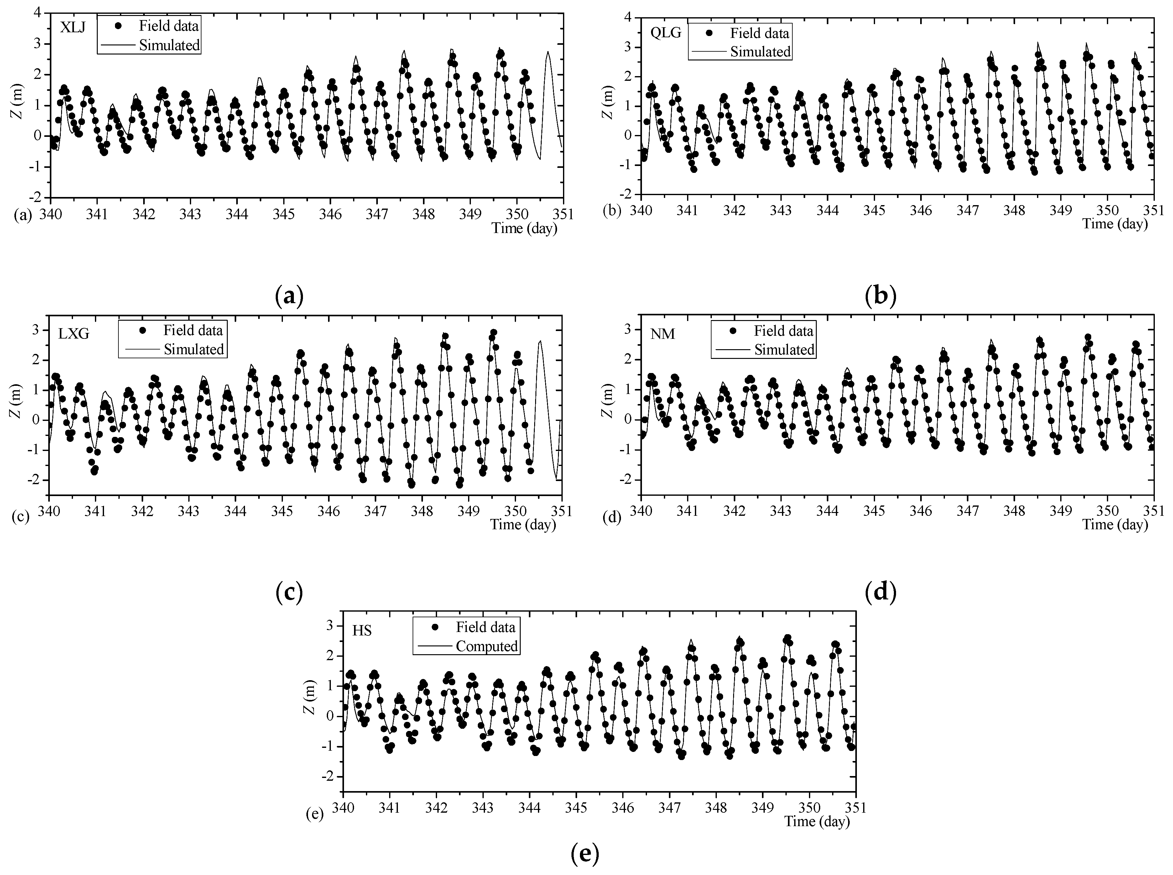
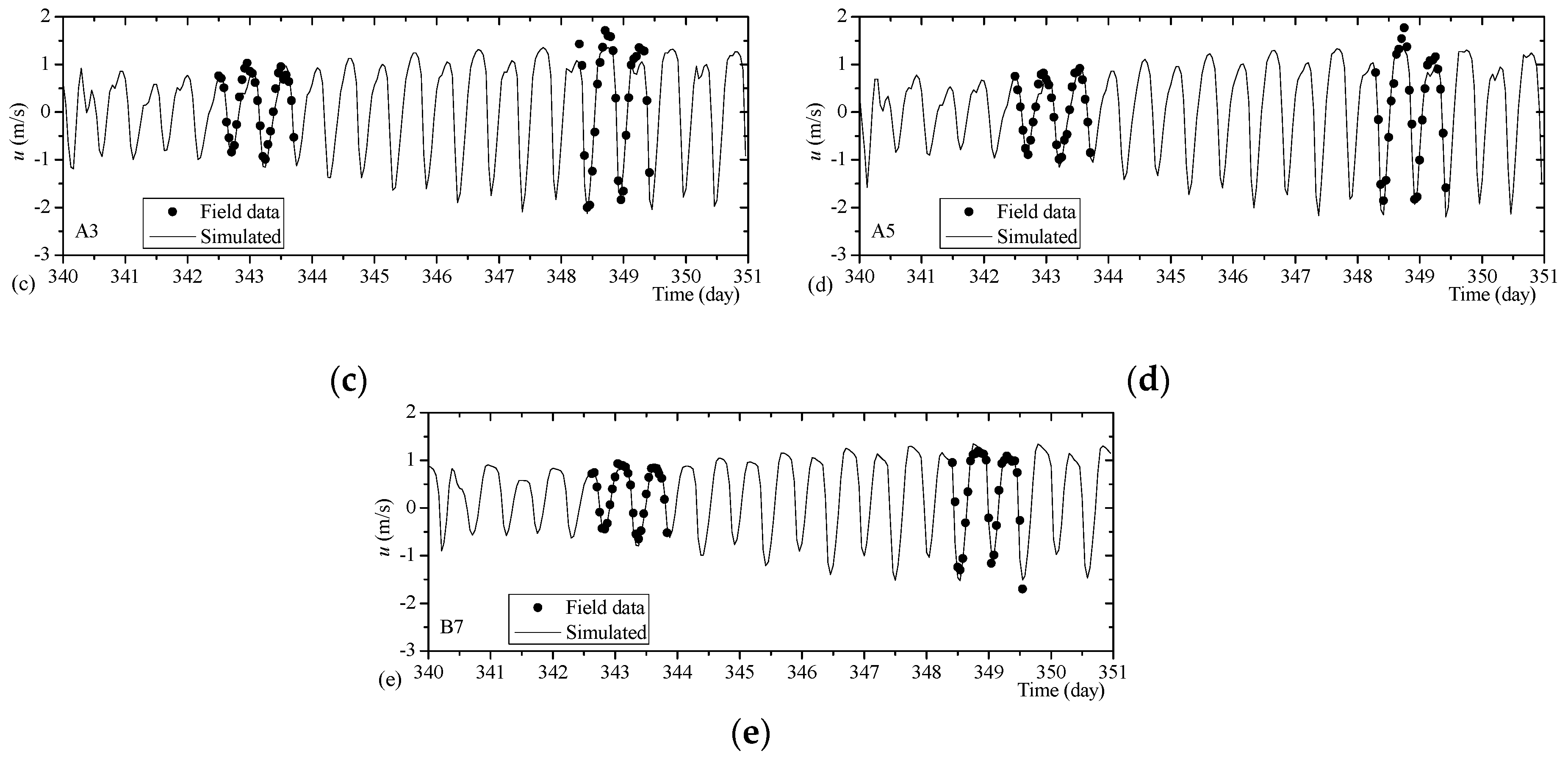
3.2. Calibration and Validation Tests of HDM
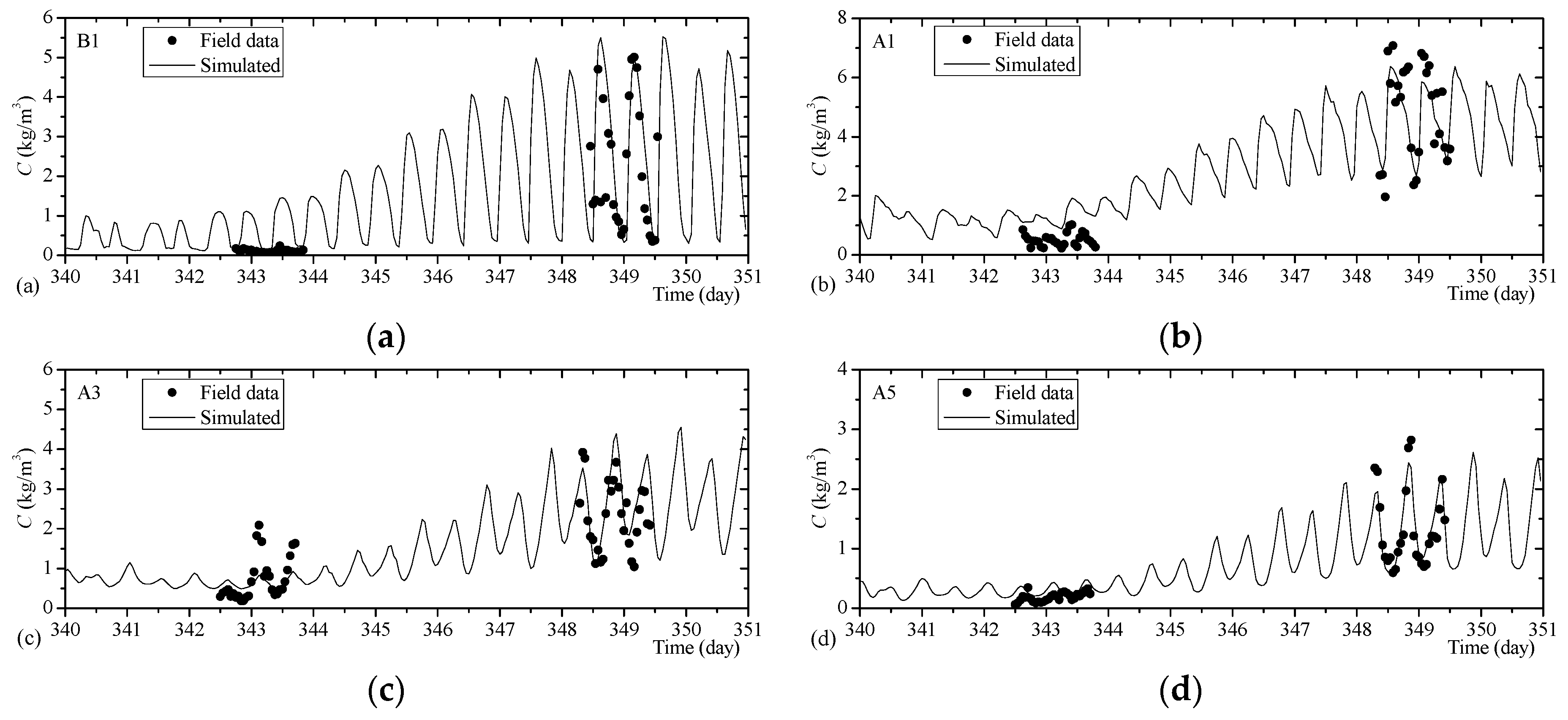
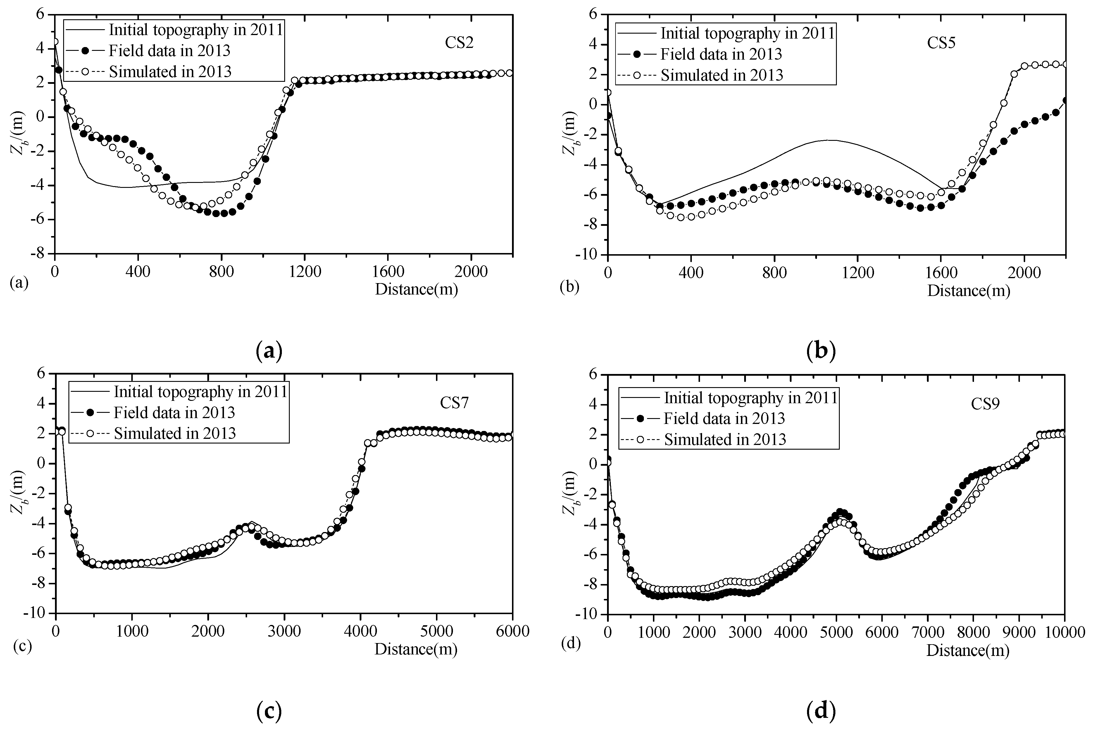
3.3. Calibration and Validation Tests of STM
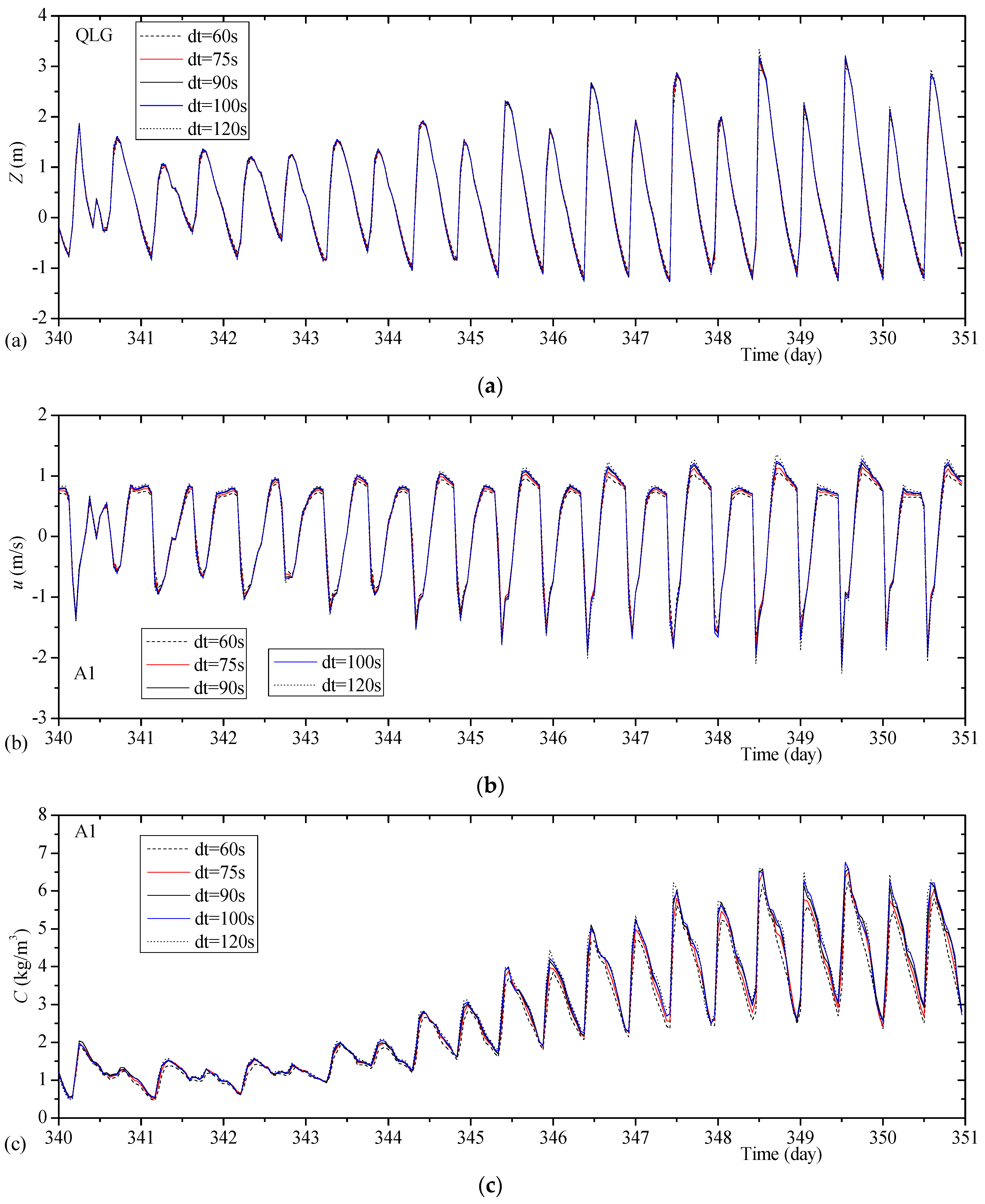
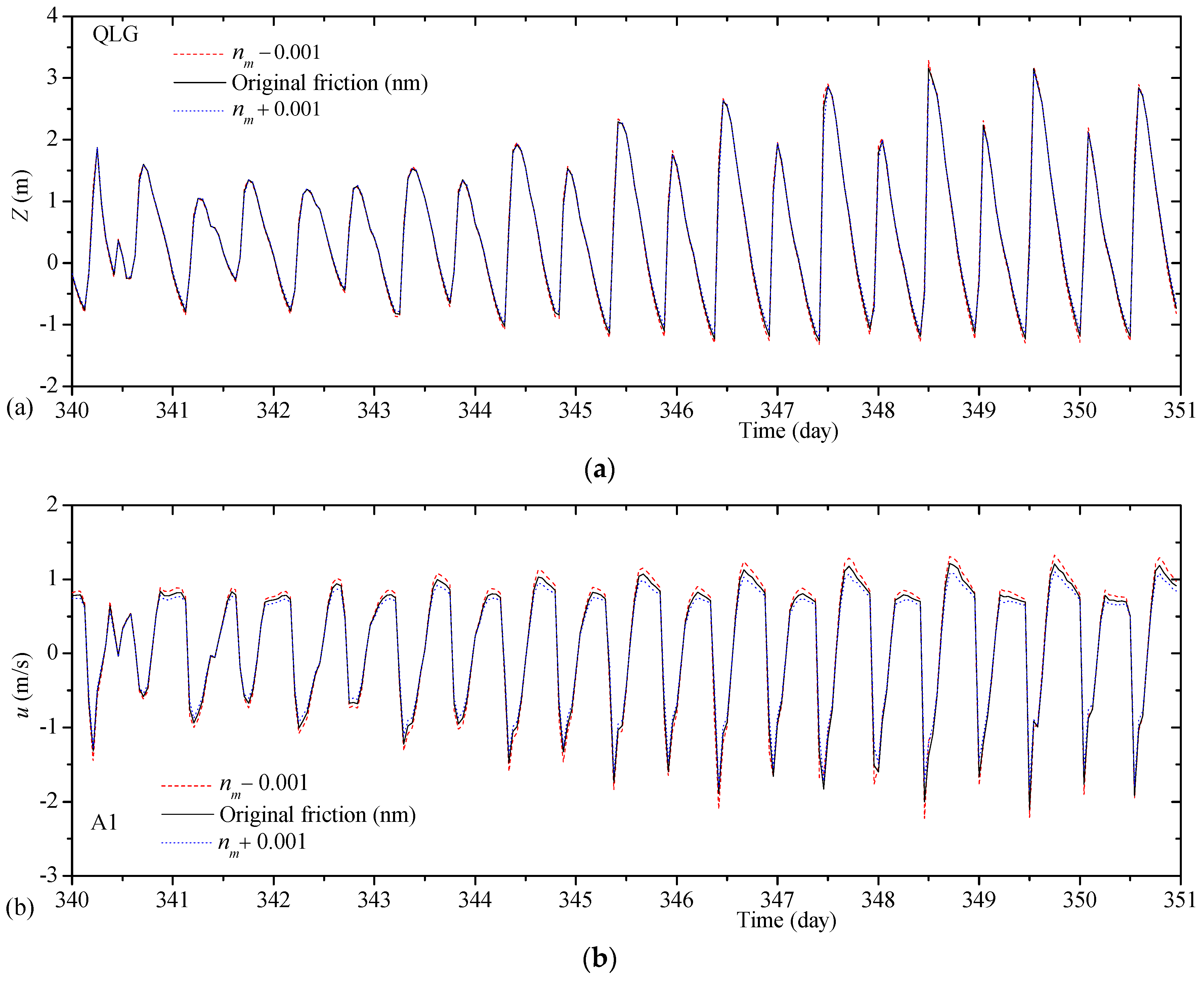
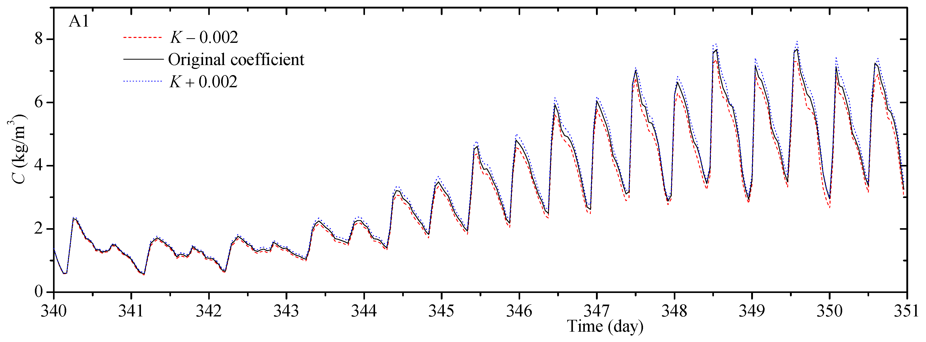
3.4. Sensitivity Study of Model Parameters and Coefficients
3.5. Efficiency Tests of HDM and STM
4. Results
4.1. Simulation Conditions
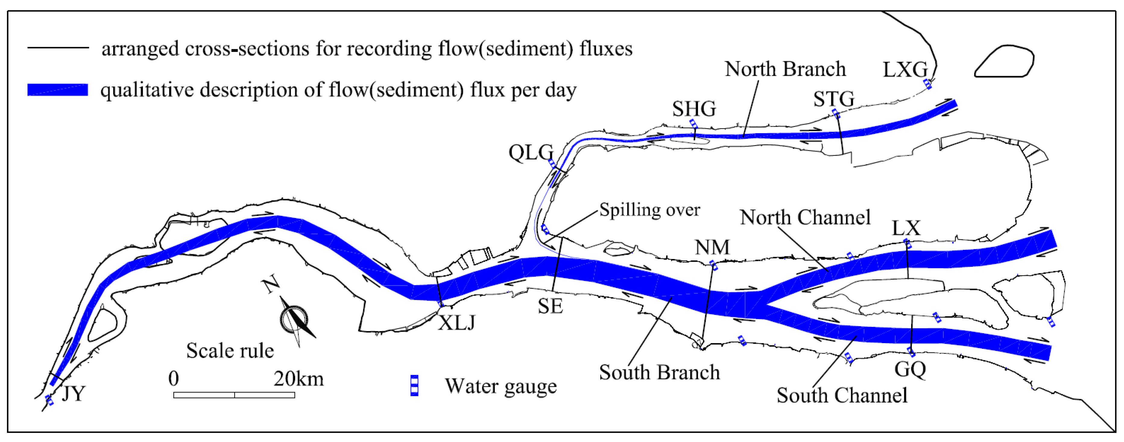
4.2. Horizontal Circulation of Water Flux
4.3. Sediment Spillover from North to South Branches
4.4. Balances of Water and Sediment Fluxes
4.5. Analysis of Spillover on Morphological Dynamics
5. Discussion
5.1. Calculation of Hydrodynamics in Estuaries
5.2. Calculation of Sediment Transport in Estuaries
5.3. Differences between the Spillover of Saltwater and Sediment
6. Conclusions
Supplementary Materials
Author Contributions
Funding
Conflicts of Interest
References
- He, S.L.; Sun, J.M. Characteristics of suspended sediment transport in the turbidity maximum of the Changjiang river estuary. Oceanol. Limnol. Sin. 1996, 27, 60–66. (In Chinese) [Google Scholar]
- Li, J.F.; Shi, W.R.; Shen, H.T. Sediment properties and transportation in the turbidity maximum in Changjiang estuary. Geogr. Res. 1994, 13, 51–59. (In Chinese) [Google Scholar]
- Shen, J.; Shen, H.T.; Pan, D.A.; Xiao, C.Y. Analysis of transport mechanism of water and suspended sediment in the turbidity maximum of the Changjiang estuary. Acta Geogr. Sin. 1995, 50, 412–420. (In Chinese) [Google Scholar]
- Shi, Z.; Chen, M.W. Fine sediment transport in turbidity maximum at the north passage of the Changjiang Estuary. J. Sediment Res. 2000, 1, 28–39. (In Chinese) [Google Scholar]
- Wu, H.; Zhu, J.R.; Chen, B.R.; Chen, Y.Z. Quantitative relationship of runoff and tide to saltwater spilling over from the North Branch in the Changjiang Estuary, A numerical study. Estuar. Coast. Shelf Sci. 2006, 69, 125–132. [Google Scholar] [CrossRef]
- Chen, W.; Li, J.F.; Li, Z.H.; Li, Z.H.; Dai, Z.J.; Yan, H.; Xu, M.; Zhao, J.K. The suspended sediment transportation and its mechanism in strong tidal reaches of the North Branch of the Changjiang Estuary. Acta Oceanol. Sin. 2012, 34, 84–91. (In Chinese) [Google Scholar]
- Chen, C.S.; Xue, P.F.; Ding, P.X.; Beardsley, R.C.; Xu, Q.C.; Mao, X.M.; Gao, G.P.; Qi, J.H.; Li, C.Y.; Lin, H.C.; et al. Physical mechanisms for the offshore detachment of the Changjiang Diluted Water in the East China Sea. J. Geophys. Res. 2008, 113. [Google Scholar] [CrossRef]
- Xue, P.F.; Chen, C.S.; Ding, P.X.; Beardsley, R.C.; Lin, H.C.; Ge, J.Z.; Kong, Y.Z. Saltwater intrusion into the Changjiang River, A model-guided mechanism study. J. Geophys. Res. 2009, 114. [Google Scholar] [CrossRef]
- Hu, D.C.; Wang, G.Q.; Zhang, H.W.; Zhong, D.Y. A semi-implicit three-dimensional numerical model for non-hydrostatic pressure free-surface flows on an unstructured, sigma grid. Int. J. Sediment Res. 2013, 28, 77–89. [Google Scholar] [CrossRef]
- Hu, K.L.; Ding, P.X.; Wang, Z.B.; Yang, S.L. A 2D/3D hydrodynamic and sediment transport model for the Yangtze Estuary, China. J. Mar. Syst. 2009, 77, 114–136. [Google Scholar] [CrossRef]
- Shi, Z.; Zhou, H.Q.; Liu, H.; Zhang, Y.C. Two-dimensional horizontal modeling of fine-sediment transport at the South Channel–North Passage of the partially mixed Changjiang River Estuary, China. Environ. Earth Sci. 2010, 61, 1691–1702. [Google Scholar] [CrossRef]
- Zuo, S.H.; Zhang, N.C.; Li, B.; Zhang, Z.; Zhu, Z.X. Numerical simulation of tidal current and erosion and sedimentation in the Yangshan deep-water harbor of Shanghai. Int. J. Sediment Res. 2009, 24, 287–298. [Google Scholar] [CrossRef]
- Kuang, C.P.; Liu, X.; Gu, J.; Guo, Y.K.; Huang, S.C.; Liu, S.G.; Yu, W.W.; Huang, J.; Sun, B. Numerical prediction of medium-term tidal flat evolution in the Yangtze Estuary, impacts of the Three Gorges project. Cont. Shelf Res. 2013, 52, 12–26. [Google Scholar] [CrossRef]
- WL|Delft Hydraulics. Delft3D-FLOW User Manual; Version 3.13; WL|Delft Hydraulics: Delft, The Netherlands, 2006. [Google Scholar]
- Wang, D.Z. Transport of Nonuniform Bedload in the Changjiang Estuary and Its Numerical Simulation. Master’s Thesis, Zhejiang University, Zhejiang, China, 2002. (In Chinese). [Google Scholar]
- Han, Q.W.; He, M.M. The Statistics Theory of Sediment Transport; Chinese Science Press: Beijing, China, 1984. (In Chinese) [Google Scholar]
- Cheng, C.; Huang, H.M.; Liu, C.Y.; Jiang, W.M. Challenges to the representation of suspended sediment transfer using a depth-averaged flux. Earth Surf. Proc. Land. 2016, 41, 1337–1357. [Google Scholar] [CrossRef]
- Dou, X.P.; Li, T.L.; Dou, G.R. Numerical model of total sediment transport in the Yangtze Estuary. China Ocean Eng. 1999, 13, 277–286. [Google Scholar]
- Wan, Y.Y.; Roelvink, D.; Li, W.H.; Qi, D.M.; Gu, F.F. Observation and modeling of the storm-induced fluid mud dynamics in a muddy-estuarine navigational channel. Geomorphology 2014, 217, 23–36. [Google Scholar] [CrossRef]
- Xie, J.; Yan, Y.X. Promoting siltation effects and impacts of Hengsha East. J. Hydrodyn. 2011, 23, 649–659. [Google Scholar] [CrossRef]
- Zhang, R.J.; Xie, J.H. River Sediment Transport; Press of Chinese Hydraulic and Electric Engineering: Beijing, China, 1989. (In Chinese) [Google Scholar]
- Wei, Z.L.; Zhao, L.K.; Fu, X.P. Research on mathematical model for sediment in Yellow River. J. Wuhan Univ. Hydr. Electr. Eng. 1997, 30, 21–25. (In Chinese) [Google Scholar]
- Zhang, Y.L.; Baptista, A.M.; Myers, E.P. A cross-scale model for 3D baroclinic circulation in estuary-plume-shelf systems, I. Formulation and skill assessment. Cont. Shelf Res. 2004, 24, 2187–2214. [Google Scholar] [CrossRef]
- Casulli, V.; Walters, R.A. An unstructured grid, three-dimensional model based on the shallow water equations. Int. J. Numer. Meth. Fluids 2000, 32, 331–348. [Google Scholar] [CrossRef]
- Hu, D.C.; Zhong, D.Y.; Zhang, H.W.; Wang, G.Q. Prediction–correction method for parallelizing implicit 2D hydrodynamic models I scheme. J. Hydraul. Eng. 2015, 141, 04015014. [Google Scholar] [CrossRef]
- Hu, D.C.; Zhong, D.Y.; Zhu, Y.H.; Wang, G.Q. Prediction–correction method for parallelizing implicit 2D hydrodynamic models II application. J. Hydraul. Eng. 2015, 141, 06015008. [Google Scholar] [CrossRef]
- Dimou, K. 3-D Hybrid Eulerian–Lagrangian/Particle Tracking Model for Simulating Mass Transport in Coastal Water Bodies. Ph.D. Thesis, Massachusetts Institute of Technology, Cambridge, MA, USA, 1992. [Google Scholar]
- Hu, D.C.; Zhu, Y.H.; Zhong, D.Y.; Qin, H. Two-dimensional finite-volume Eulerian-Lagrangian method on unstructured grid for solving advective transport of passive scalars in free-surface flows. J. Hydraul. Eng. 2017, 143, 04017051. [Google Scholar] [CrossRef]
- Cheng, Y.C.; Andersen, O.B.; Knudsen, P. Integrating non-tidal sea level data from altimetry and tide gauges for coastal sea level prediction. Adv. Space Res. 2012, 50, 1099–1106. [Google Scholar] [CrossRef]
- Wu, S.H.; Cheng, H.Q.; Xu, Y.J.; Li, J.F.; Zheng, S.W.; Xu, W. Riverbed micromorphology of the Yangtze River Estuary, China. Water 2016, 8, 190. [Google Scholar] [CrossRef]
- Cao, Z.Y. A Two-Dimensional Non-Uniform Sediment Numerical Model for the Yangtze Estuary. Ph.D. Thesis, East China Normal University, Shanghai, China, 2003. (In Chinese). [Google Scholar]
- Shi, Y.B.; Lu, H.Y.; Yang, Y.P.; Cao, Y. Prediction of erosion depth under the action of the exceptional flood in the river reach of a tunnel across the Qiantang estuary. Adv. Water Sci. 2008, 19, 685–692. (In Chinese) [Google Scholar]
- Baptista, A.M. Solution of Advection-Dominated Transport by Eulerian–Lagrangian Methods Using the Backwards Method of Characteristics. Ph.D. Thesis, Massachusetts Institute of Technology, Cambridge, MA, USA, 1987. [Google Scholar]
- Hu, D.C.; Zhang, H.W.; Zhong, D.Y. Properties of the Eulerian-Lagrangian method using linear interpolators in a three dimensional shallow water model using z-level coordinates. Int. J. Comput. Fluid Dyn. 2009, 23, 271–284. [Google Scholar] [CrossRef]
- Li, Z.H.; Li, M.Z.; Dai, Z.J.; Zhao, F.F.; Li, J.F. Intratidal and neap-spring variations of suspended sediment concentrations and sediment transport processes in the North Branch of the Changjiang Estuary. Acta Oceanol. Sin. 2015, 34, 137–147. [Google Scholar] [CrossRef]
- Liu, H.; He, Q.; Wang, Z.B.; Weltje, G.J.; Zhang, J. Dynamics and spatial variability of near-bottom sediment exchange in the Yangtze Estuary, China. Estuar. Coast. Shelf Sci. 2010, 86, 322–330. [Google Scholar] [CrossRef]
- Shi, Z.; Zhang, S.Y.; Hamilton, L.J. Bottom fine sediment boundary layer and transport processes at the mouth of the Changjiang Estuary, China. J. Hydrol. 2006, 327, 276–288. [Google Scholar] [CrossRef]
- Yang, S.L.; Belkinb, I.M.; Belkinac, A.I.; Zhao, Q.Y.; Zhu, J.; Ding, P.X. Delta response to decline in sediment supply from the Yangtze River: Evidence of the recent four decades and expectations for the next half-century. Estuar. Coast. Shelf Sci. 2003, 57, 689–699. [Google Scholar] [CrossRef]
- Tan, Y.; Yang, F.; Xie, D.H. The change of tidal characteristics under the influence of human activities in the Yangtze Estuary. J. Coast. Res. 2016, 75, 163–167. [Google Scholar] [CrossRef]
- Wu, D.; Shao, Y.; Pan, J. Study on activities and concentration of saline group in the South Branch in Yangtze River Estuary. Procedia Eng. 2015, 116, 1085–1094. [Google Scholar]
- Lu, S.; Tong, C.; Lee, D.Y.; Zheng, J.; Shen, J.; Zhang, W.; Yan, Y. Propagation of tidal waves up in Yangtze Estuary during the dry season. J. Geophys. Res. Oceans 2015, 120, 6445–6473. [Google Scholar] [CrossRef]
- Ge, J.Z.; Ding, P.X.; Chen, C.S. Low-salinity plume detachment under non-uniform summer wind off the Changjiang Estuary. Estuar. Coast. Shelf Sci. 2015, 156, 61–70. [Google Scholar] [CrossRef]
- Hou, C.C.; Zhu, J.R. The response time of saltwater intrusion in the Changjiang River to the change of river discharge in dry season. Acta Oceanol. Sin. 2013, 35, 29–35. (In Chinese) [Google Scholar]
- An, Q.; Wu, Y.Q.; Taylor, S.; Zhao, B. Influence of the Three Gorges Project on saltwater intrusion in the Yangtze River Estuary. Environ. Geol. 2009, 56, 1679–1686. [Google Scholar] [CrossRef]
- Zhang, J.X.; Liu, H. Numerical investigation of pollutant transport by tidal flow in the Yangtze Estuary. In Trends in Engineering Mechanics Special Publication; Huang, W., Wang, K., Chen, Q., Eds.; American Society of Civil Engineers: Los Angeles, CA, USA, 2010; pp. 99–110. [Google Scholar]
- Kuang, C.P.; Chen, W.; Gu, J.; He, L.L. Comprehensive analysis on the sediment siltation in the upper reach of the deepwater navigation channel in the Yangtze Estuary. J. Hydrodyn. 2014, 26, 299–308. [Google Scholar] [CrossRef]
- Zhang, S.; Duan, J.; Strelkoff, T. Grain-scale nonequilibrium sediment-transport model for unsteady flow. J. Hydraul. Eng. 2012, 139, 22–36. [Google Scholar] [CrossRef]
- Xia, J.Q.; Lin, B.L.; Falconer, R.A.; Wang, G.Q. Modelling dam-break flows over mobile beds using a 2D coupled approach. Adv. Water Res. 2010, 33, 171–183. [Google Scholar] [CrossRef]
- Wu, W.M. Earthen embankment breaching. J. Hydraul. Eng. 2011, 137, 1549–1564. [Google Scholar]
- Cao, Z.; Pender, G.; Wallis, S.; Carling, P. Computational dam-break hydraulics over erodible sediment bed. J. Hydraul. Eng. 2004, 130, 689–703. [Google Scholar] [CrossRef]
- Gu, Y.; Wu, S.; Yue, Q. Impact of intruded saline water via North Branch of the Yangtze River on water source areas in the estuary area. Yangtze River 2003, 34, 1–16. (In Chinese) [Google Scholar]


| Region | Length (km) | Area (km2) | Resolution of Bathymetry Graph | Grid Scale (m × m) |
|---|---|---|---|---|
| Tidal reach | 533 | 2066 | 1/10,000 | 200 × 80 |
| North Branch | 80 | 366 | 1/10,000 | 200 × 80–400 × 200 |
| South Branch | 88 | 1132 | 1/25,000 | 400 × 200 |
| Coast region | - | 8746 | - | 500–2000 |
| East Sea | - | 105,993 | - | 2000–5000 |
| Region | Cross-Section | Spring Tide | Neap Tide | ||
|---|---|---|---|---|---|
| Flood | Ebb | Flood | Ebb | ||
| River | JY | −7.72 1 | 24.20 | −3.25 | 19.68 |
| XLJ | −28.26 | 44.57 | −15.03 | 31.39 | |
| North Branch | QLG | −2.48 | 1.88 | −1.63 | 1.16 |
| SHG | −5.73 | 5.14 | −3.22 | 2.76 | |
| STG | −11.06 | 10.48 | −6.26 | 5.80 | |
| South Branch | SE | −31.41 | 48.35 | −16.34 | 33.18 |
| NM | −38.79 | 55.64 | −18.96 | 35.82 | |
| North C. | −28.52 | 36.05 | −13.09 | 21.15 | |
| South C. | −25.32 | 34.61 | −11.36 | 20.21 | |
| Region | Cross-Section | Spring Tide | Neap Tide | ||
|---|---|---|---|---|---|
| Flood | Ebb | Flood | Ebb | ||
| River | JY | −10.62 1 | 33.92 | −3.31 | 20.60 |
| XLJ | −55.76 | 81.11 | −15.28 | 30.76 | |
| North Branch | QLG | −116.73 | 72.88 | −32.28 | 21.02 |
| SHG | −244.80 | 204.47 | −56.09 | 50.97 | |
| STG | −190.93 | 198.84 | −42.65 | 46.96 | |
| South Branch | SE | −85.76 | 142.00 | −19.33 | 42.69 |
| NM | −157.33 | 218.09 | −31.61 | 57.77 | |
| North C. | −130.29 | 164.43 | −20.87 | 36.27 | |
| South C. | −82.05 | 109.83 | −13.83 | 25.29 | |
© 2019 by the authors. Licensee MDPI, Basel, Switzerland. This article is an open access article distributed under the terms and conditions of the Creative Commons Attribution (CC BY) license (http://creativecommons.org/licenses/by/4.0/).
Share and Cite
Hu, D.; Wang, M.; Yao, S.; Jin, Z. Study on the Spillover of Sediment during Typical Tidal Processes in the Yangtze Estuary Using a High-Resolution Numerical Model. J. Mar. Sci. Eng. 2019, 7, 390. https://doi.org/10.3390/jmse7110390
Hu D, Wang M, Yao S, Jin Z. Study on the Spillover of Sediment during Typical Tidal Processes in the Yangtze Estuary Using a High-Resolution Numerical Model. Journal of Marine Science and Engineering. 2019; 7(11):390. https://doi.org/10.3390/jmse7110390
Chicago/Turabian StyleHu, Dechao, Min Wang, Shiming Yao, and Zhongwu Jin. 2019. "Study on the Spillover of Sediment during Typical Tidal Processes in the Yangtze Estuary Using a High-Resolution Numerical Model" Journal of Marine Science and Engineering 7, no. 11: 390. https://doi.org/10.3390/jmse7110390
APA StyleHu, D., Wang, M., Yao, S., & Jin, Z. (2019). Study on the Spillover of Sediment during Typical Tidal Processes in the Yangtze Estuary Using a High-Resolution Numerical Model. Journal of Marine Science and Engineering, 7(11), 390. https://doi.org/10.3390/jmse7110390