Article

Lateral Circulation in a Partially Stratified Tidal Inlet

Department of Oceanography and Coastal Sciences, College of the Coast and Environment, Louisiana State University, Baton Rouge, LA 70803, USA
*
Author to whom correspondence should be addressed.
J. Mar. Sci. Eng. 2018, 6(4), 159; https://doi.org/10.3390/jmse6040159
Submission received: 30 September 2018 / Revised: 27 November 2018 / Accepted: 3 December 2018 / Published: 19 December 2018

Abstract

:
Using a three-dimensional, hydrostatic, primitive-equation ocean model, this study investigates the dynamics of lateral circulation in a partially stratified tidal inlet, the Barataria Pass in the Gulf of Mexico, over a 25.6 h diurnal tidal cycle. Model performance is assessed against observational data. During flood tide, the lateral circulation exhibits the characteristics similar to those induced by differential advection, i.e., lateral flow consists of two counter-rotating cells and is convergent at the surface. The analysis of momentum balance indicates that, in addition to the pressure gradient and vertical stress divergence, nonlinear advection and horizontal stress divergence are also important contributors. During ebb phase, the lateral circulation is mostly toward the right shoal (when looking into the estuary) for the whole water column and persisting for almost the whole period. The surface divergence suggested by the differential advection mechanism lasts for a very short period, if it ever exists. The main momentum balance across most of the transect during ebb is between the along-channel advection of cross-channel momentum and pressure gradient. The sectional averaged lateral velocity magnitude during ebb is comparable to that during flood, which is different from the idealized numerical experiment result.

1. Introduction

The lateral circulation in tidally dominant estuaries can be driven by various mechanisms. Nunes and Simpson [1] identified the effect of differential advection on the generation of secondary circulation. They pointed out that due to frictional retardation, the along-channel velocity is stronger in the channel than over the shoals. When acting upon an along-channel density gradient, it results in greater (smaller) density at the thalweg than at the shoals during flood (ebb) tides. This produces a cross-channel pressure gradient toward the channel (shoals) on the surface and a pressure gradient toward the shoals (channel) at the bottom during flood (ebb) tides. Thus, the lateral flows are convergent (divergent) at the surface over the deep channel and divergent (convergent) at the bottom during flood (ebb) tides. However, the surface axial convergence was only observed during flood tides in Nunes and Simpson’s work.
In an idealized, narrow straight channel with weak stratification, Lerczak and Geyer [2] confirmed that secondary circulation was driven by differential advection. Differential rotation of tidal ellipse was also identified as a mechanism for axial convergence fronts [3]. Interactions between barotropic pressure gradient and bathymetry can generate convergence of lateral flow, producing flows rotating toward the channel from the shoals [4,5]. In curved estuaries, an alternative driving mechanism for lateral circulation is the centrifugal acceleration [6,7,8] and advection [9]. Winds can enhance or degrade the local-curvature-induced, two-layer flow and can drive three-layer flow [10]. Ekman-forced lateral circulation varies with the Ekman number. When the boundary layer is comparable to the channel depth (large Ekman number), lateral flow is a single circulation cell; while for thin tidal boundary layer (small Ekman number), lateral flow is complex and varies over the tidal cycle [2]. Boundary mixing on a no-flux boundary layer was confirmed to be one of the driving mechanisms of lateral circulation [2,11]. Cheng et al. [12] investigated the lateral circulation during stratified ebb tides due to the lateral baroclinic pressure gradient, which is generated by differential diffusion caused by a lateral asymmetry in vertical mixing.
In the same idealized numerical experiment, Lerczak and Geyer [2] found that lateral flow is about four times stronger during flood tides than during ebb tides. They attributed it to the interaction between the along-channel tidal currents and nonlinear advective processes over a tidal cycle. This flood–ebb asymmetry in the lateral circulation strength was also observed by Scully et al. [13] in the Hudson River estuary, where stronger lateral flows were observed during flood tides while lateral flows were suppressed during ebb tides. However, in the numerical modeling of James River Estuary, Li et al. [14] found flood–ebb asymmetry during neap tides with stronger lateral circulation on ebb, while flood–ebb asymmetry was reduced during spring tides.
Lateral circulation plays an important role in estuarine dynamics. Many observational and numerical simulation results [2,7,12,15,16] have demonstrated the existence of secondary currents, and discussed its dependence and feedback on density stratification [7,12,17,18], streamwise momentum budget [2], estuarine circulation [12,13], as well as its impacts on sediment transport and geomorphology [19,20,21]. In Barataria Pass, the area of focus for this study, observations showed that there existed a distinct asymmetry in stratification within the diurnal cycle [22]. However, in that analysis no consideration was given to the contribution of the lateral circulation to density stratification.
In this study, we use a three-dimensional (3-D), high-resolution hydrodynamic model to examine the lateral circulation structure in the partially stratified tidal inlet, Barataria Pass, which connects Barataria Bay with the continental shelf in the southeastern Louisiana. The objectives of this study are to elucidate the tidal evolution of lateral circulation and determine its driving mechanisms. The remainder of this paper is organized as follows: Section 2 describes the study area, and the configuration of the 3-D finite volume numerical ocean model. Section 3 presents the validation of the numerical model and the temporal evolution of lateral circulation over a 25.6 h diurnal tidal cycle. In Section 4, we quantify the 2-D and 3-D momentum balance and examine the driving forcing for lateral circulation. Flood–ebb variations in lateral circulation pattern are also discussed in Section 4. Finally, conclusions are given in Section 5.

2. Materials and Methods
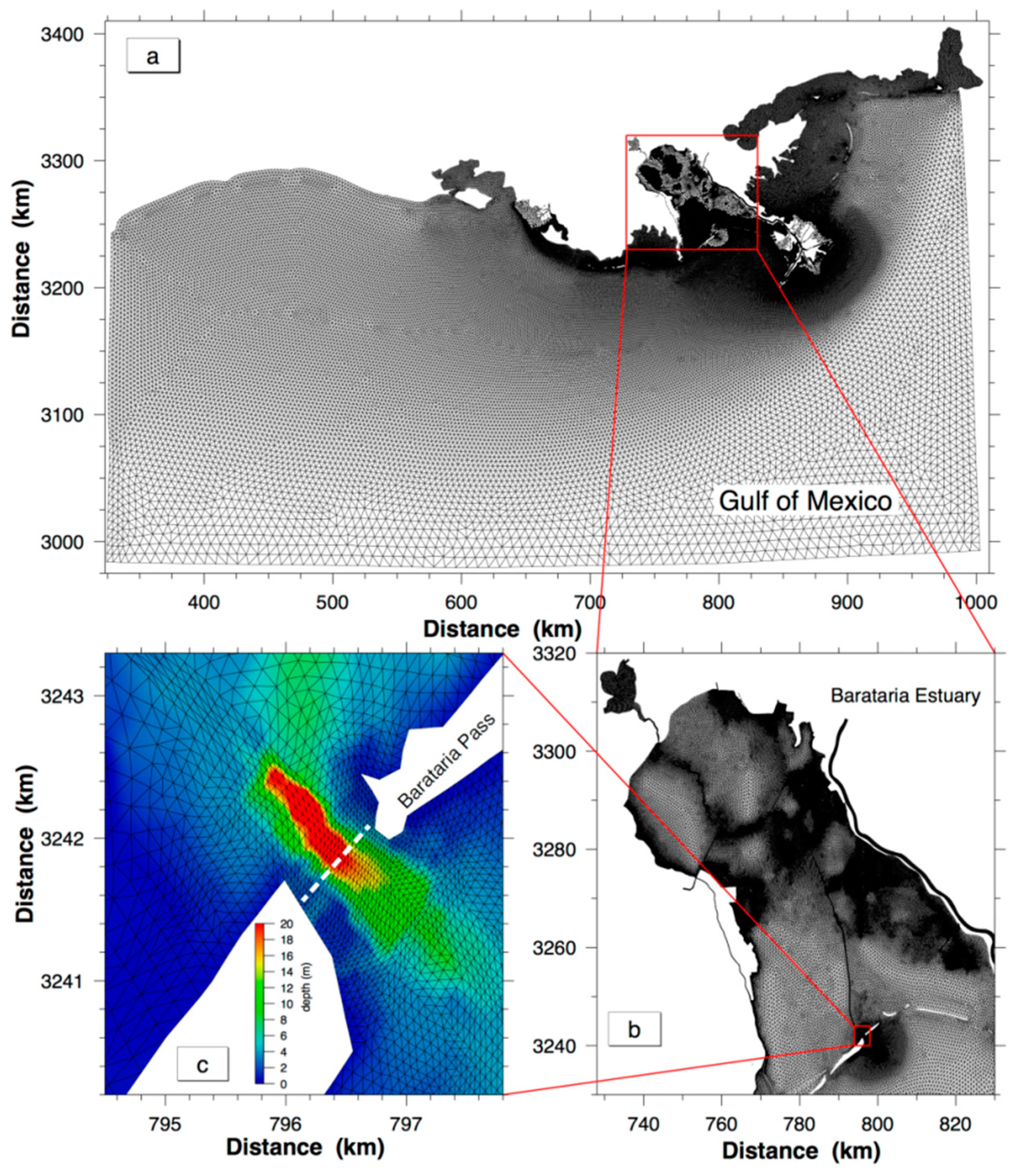
2.1. Study Area

Barataria Bay (Figure 1) is located at the southeastern Louisiana, on the western side of the Mississippi Birdfoot Delta. It is connected to the Gulf of Mexico through several tidal inlets including Barataria Pass, which is between two barrier islands, Grand Isle Island and Grand Terre Island (Figure 1b). The most significant freshwater source inside the Barataria Bay is the Davis Pond freshwater diversion. The maximum diversion discharge is ~300 m3 s−1 [23]. Barataria Pass is an 800 m wide narrow channel. It is one of the four main tidal passes of Barataria Bay, accounting for ~66% of total water exchange [24]. Tidal currents account for ~85% of the total flow variance in the inlet, with equal contributions from the O1 and K1 constituents. Tidal amplitudes for both O1 and K1 constituents are about 0.5 m s−1 [25]. Maximum tidal currents reach as high as 2 m s−1 during tropic tides.
Barataria Bay is composed of broad shallow waters (average depth of 2 m), islands and a 5 m deep main shipping channel, the Barataria Waterway. The shipping channel ends at Barataria Pass. Around Barataria Pass the main channel has an average depth of ~20 m and is being periodically dredged, causing a depression of ~50 m deep close to the inlet (Figure 2). A cross-sectional view of the Barataria Pass, along which all analyses are performed, is shown in Figure 1c. Bathymetrically this transect has one 20 m deep channel in the center bordered by extensive shoal regions. The shoal at the left-hand side (looking upstream) is ~2 m deep and 250 m wide, while that at the right-hand side is ~3 m deep and 100 m wide.

2.2. Model Description and Configuration

The Finite Volume Coastal Ocean Model (FVCOM) is used in this study to simulate the hydrodynamics of the Barataria Basin and adjacent continental shelf. FVCOM is a 3-D, hydrostatic, free surface, primitive-equation ocean model [26,27]. In the finite volume method, the computational domain is discretized using a mesh of non-overlapping triangles in the horizontal and sigma-coordinate (σ-coordinate) in the vertical. The governing equations are solved in their integral forms in each individual control volume. The triangular grid in the horizontal can resolve complex coastal and bathymetric geometries. It uses a cell-vertex-centered (similar to the finite-difference C-grid) method, which facilitates the enforcement of mass conservation in tracer advection and tracer open boundary conditions. Vertical mixing uses modified Mellor and Yamada level 2.5 turbulence model [28,29] and horizontal diffusion uses Smagorinsky eddy parameterization [30]. The model employs mode split approaches (barotropic 2D (external) mode and baroclinic 3D (internal) mode) to solve the momentum equations with second-order accuracy. The bottom boundary conditions apply an exact form of the no flux boundary conditions.
A flooding–drying scheme is implemented in FVCOM to simulate motions in intertidal zones and wetlands. If vertical water column thickness at the cell center is less than a criterion value (typically 5 cm), then the cell is designated as a dry cell and its velocity is set to zero. Whenever the vertical water column thickness exceeds the criterion value, the cell becomes wet and water level and velocity are computed from control equations. The advantage of triangular mesh to accurately represent complex bathymetry and coastlines makes FVCOM ideally suited for Barataria Pass study.
A high-resolution FVCOM Barataria Pass model was developed by configuring FVCOM version 2.6 to the Northwestern Gulf of Mexico continental shelf region with inclusion of the intertidal zones inside the Barataria Bay. The computational domain extends longitudinally from Mobile Bay (Alabama) to west of Galveston Bay (Texas) and offshore to about 27° N (Figure 2). It consists of 146,266 triangular nodes and 283,721 triangular cells. The horizontal grid resolution varies from about 10 m in the upper estuary to about 8 km near the open boundary. Near Barataria Pass, grid cells are fine enough to ensure that the 800 m wide inlet cross section is resolved by ~20 triangles (Figure 2c). Vertically FVCOM employs 19 uniform sigma layers, which is ~0.1 m over the shoal and ~1 m in the central depression of the tidal inlet. Computational time steps are 0.2 s and 2.0 s for the external and internal modes, respectively. Model results are saved every 10 min for further diagnostic analysis.
Model bathymetry was obtained from various sources. Using an inverse distance weighted interpolation method, a 5 m by 5 m resolution digital elevation model constructed from Light Detection and Ranging (LIDAR) measurement was interpolated into model wetland region. The water depth in channels, bayous, and lakes was interpolated from Coastal Louisiana Ecosystem Assessment and Restoration Report (CLEAR), US Army Corp Survey, and NOAA nautical charts. Shelf and open ocean water depth was interpolated from a coarse resolution ADCIRC model bathymetry. The water depth values in the inlet were obtained by vessel-based surveys [22,31].
Since temperature difference is minute across much of our modeling region during summer time [32], salinity is considered to be the most important factor that influences water density and vertical stratification in Barataria Bay and adjacent coastal oceans in this study. Thus it is the only prognostic tracer variable in FVCOM simulations. Temperature is kept as a spatial and temporal constant (20 °C). The coefficients for horizontal viscosity and diffusivity are both set to be 0.4 m2 s−1. The conventional quadratic bottom friction formulation is applied, with drag coefficient Cd determined by matching a logarithmic bottom boundary layer velocity to that of the numerical model at the lowest sigma-layer height. However, bottom drag coefficient over the wetlands is defined as five times greater than that in the estuarine channels, mimicking the vegetation damping effect [33].

2.3. Model Forcing, Initial, and Boundary Conditions

FVCOM is driven by winds at the surface, sea level elevation at the open boundary, and freshwater inflows from various Mississippi River and Atchafalaya River passes, and the Davis Pond Diversion. It is initialized on 1 October 2007 and run until 31 December 2008. We use 3-hourly wind data from NOAA National Centers for Environmental Prediction (NCEP) North American Regional Reanalysis (NARR) products and interpolate it onto the entire computational domain. The initial values of sea level elevation and velocity are specified as zero throughout the computational domain. The initial salinity field over the continental shelf is interpolated from HYCOM Gulf of Mexico 1/25° reanalysis product, while salinity inside the Barataria Bay is interpolated from observations at the United States Geological Survey (USGS) stations. Experiments show that this technique gives more accurate salinity simulation result than that with linear interpolation from estuarine head to the mouth. At the open boundary, the 6-min interval sea level time series at four stations are downloaded from NOAA tides and currents website. Time series of Dauphin Island, Southwest Pass, Freeport, and Galveston Pier 21 are directly used to prescribe sea surface elevations at the easternmost node, the southeastern node, the southwestern node, and the westernmost node, respectively. Sea level elevation at other open boundary nodes are piecewise linearly interpolated from these four nodes. Observed 15-min freshwater discharge at four locations, Mississippi River at Belle Chasse, David Pond diversion, Atchafalaya River at Morgan City, and Wax Lake Outlet, are injected into the computational domain with flux boundary conditions of zero salinity and specified volume and momentum. All model forcing functions are ramped up from zero over a period of 10 days.

2.4. Observations

Simulated water elevation, velocity and salinity are compared with in situ observations. Water elevation data is obtained from National Water Information System of USGS shown in Figure 1, including six stations, Barataria Bay near Grand Terre Island (S1), Barataria Bay North of Grand Isle (S2), Hackberry Bay near NW of Grand Isle (S3), Barataria Waterway (S4), Little Lake near Bay Dosgris (S5), and Little Lake near Bay Cutoff (S6). The unit of water elevation is converted to meter and vertical datum is adjusted to mean sea level in order to be compared with model results. Velocity and salinity data are from the field observations conducted at Barataria Pass from 11:30 31 July to 11:10 1 August 2008 UTC (see Li et al. [31] for details about field observation and data processing).

2.5. Analysis Methods

The vertically averaged cross- and along-channel momentum equations are written as:
1 D u ¯ D t = 1 D ( u ¯ 2 D x + u ¯ v ¯ D y ) + f v ¯ g ζ x g ρ 0 [ 1 0 x ( D σ 0 ρ d σ ) d σ + D x 1 0 σ ρ d σ ] + τ s x D ρ 0 τ b x D ρ 0 + F x ˜ + 1 D G x
1 D v ¯ D t D D T = 1 D ( u ¯ v ¯ D x + v ¯ 2 D y ) A D V f u ¯ C O R g ζ y D P B P g ρ 0 [ 1 0 y ( D σ 0 ρ d σ ) d σ + D y 1 0 σ ρ d σ ] D P B C + τ s y D ρ 0 W I N D τ b y D ρ 0 F R I C + F y ˜ H D I F + 1 D G y A V 2 D
where ( u ¯ , v ¯ ) are the vertical integrated cross- and along-axis velocity components. The positive u is pointed to the eastern bank, the positive v to the upstream. Terms from the left to the right are local acceleration (DDT), nonlinear advection (ADV), Coriolis force (COR), barotropic pressure gradient (DPBP), baroclinic pressure gradient (DPBC), wind stress (WIND), bottom friction (FRIC), horizontal diffusion (HDIF), and difference between nonlinear terms of vertically-averaged 2-D variables and vertical integration of 3-D variables (AV2D). The expressions for HDIF and AV2D can be referred to [26,27]. Consistent with 3-D currents converted to cross- and along-channel directions, all terms in Equations (1) and (2) are rotated from the original FVCOM computation x-y coordinates (see Appendix A for details).
A 3-D FVCOM momentum equation analysis was used to identify the mechanisms that drive lateral circulation. The equation is written as:
1 D u D t = 1 D u 2 D x 1 D u v D y 1 D u ω σ + f v g ζ x g ρ 0 [ x ( D σ 0 d σ + σ ρ D x ) ] + 1 D 2 σ ( K m u σ ) + F x
1 D v D t D D T = 1 D u v D x A D V U 1 D v 2 D y A D V V 1 D v ω σ A D V W f u C O R g ζ y D P B P g ρ 0 [ y ( D σ 0 d σ + σ ρ D y ) ] D P B C + 1 D 2 σ ( K m v σ ) V D I F + F y H D I F
where ( u , v ) are cross- and along-channel velocity components. The advection terms are moved to the same side of the pressure gradient, and each term in Equations (3) and (4) is calculated with its corresponding sign (e.g., ( u 2 D ) / D x ).

3. Results

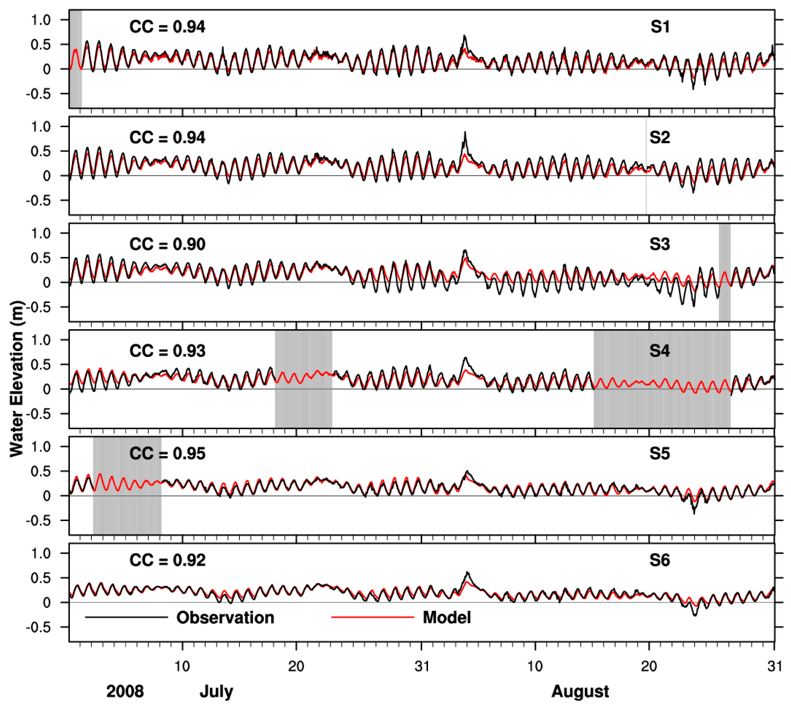
3.1. Two-Month Water Elevation Comparisons
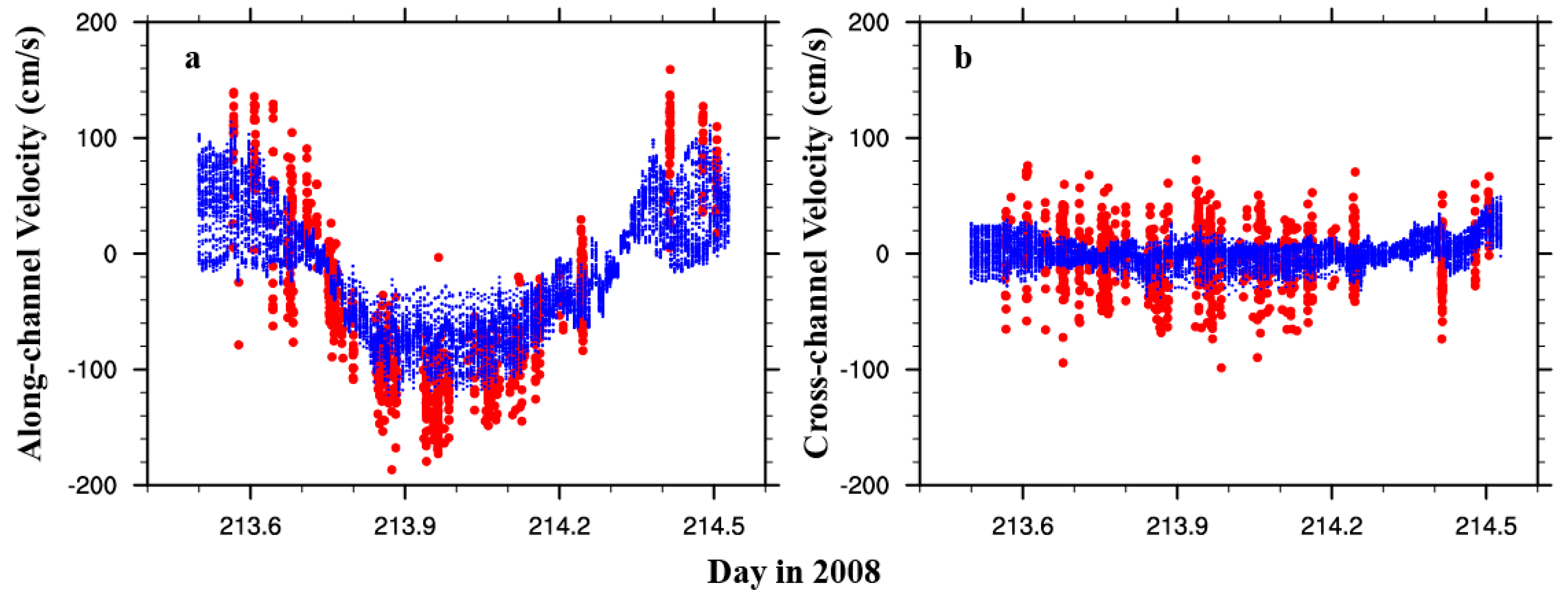
We use the Pearson correlation coefficient [34] as evaluation metrics. Two-month (1 July to 31 August 2008) time series of water elevation for both observation and model simulation are shown in Figure 3. The model reproduces the observed tidal variations, including tropic-equatorial modulation, as well as wind-driven water level set-up and set-down with all correlation coefficients above 0.9.

3.2. Velocity

Similar to the treatment in Li et al. [22], the x- and y-velocity components were counterclockwise rotated by 52.7° from the east and north direction to obtain the cross- and along-channel velocity components (Figure 1b), which are shown in Figure 4. Positive along-channel velocity is flood current. As shown in Figure 4a, the observed along-channel velocity has a stronger tidal signal, with maximum magnitude of ~1.5 m s−1, than the model simulated velocity, which has a maximum magnitude of ~1.0 m s−1. The tidal phase is in agreement with the observations. Both observed and modeled cross-channel velocities (Figure 4b) are much smaller and noisier, and the tidal signal is not clear compared to the along channel velocity component. The discrepancy between the observed and modeled velocity is, in part, due to the fact that observed velocity data points were chosen along a 530 m long transect within a 90 m band (45 m on each side [22]), while modeled velocity data points are exactly along the chosen transect.

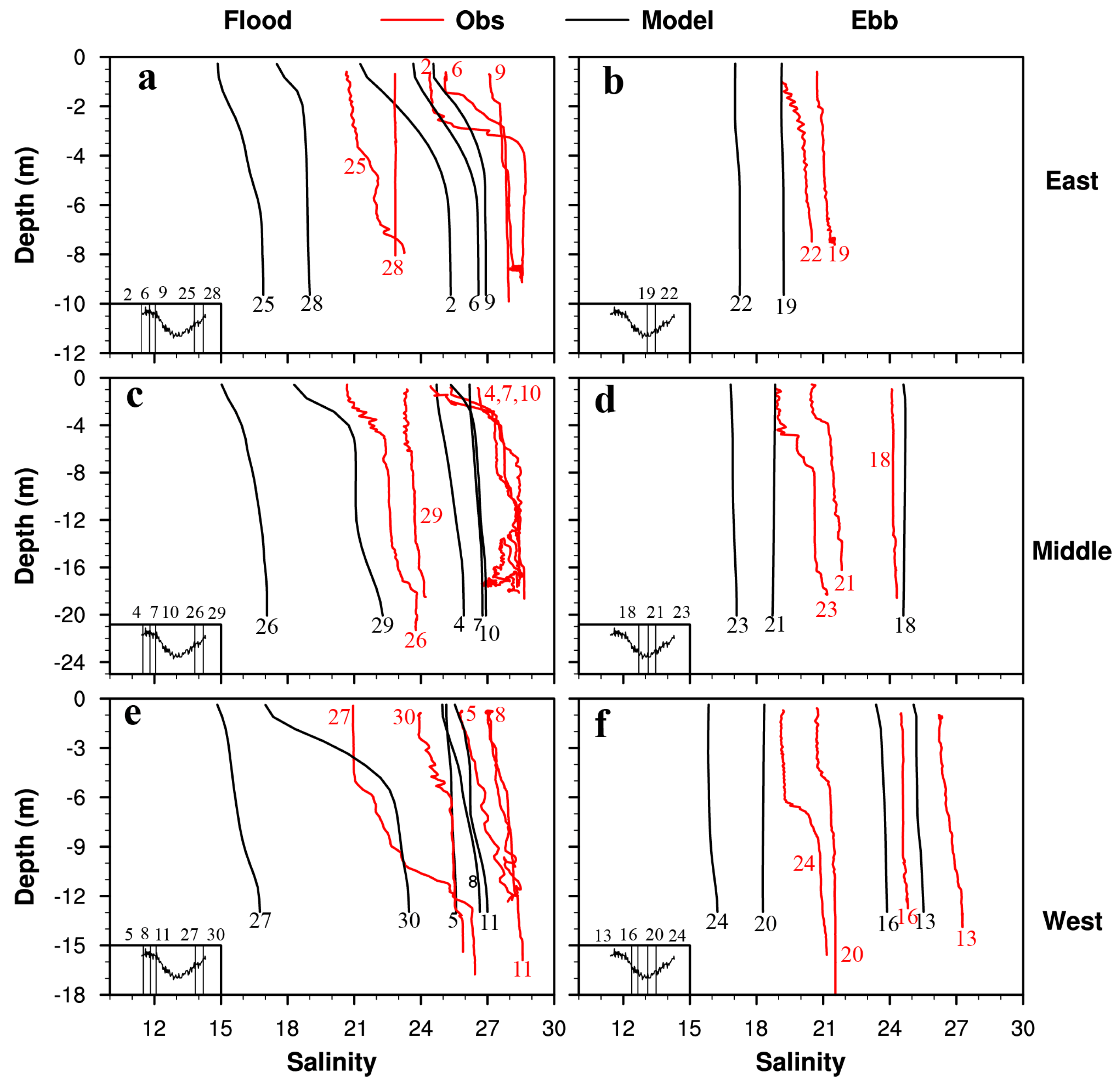
3.3. Vertical Salinity Profile

A seabird Electronics Conductivity, Temperature, and Depth Sensor (CTD) was used for vertical profiles of salinity. A total of 28 CTD casts were made between 31 July and 1 August 2008 over a 25.6 h period (see Table 1 in Li et al. [31] for details). Vertical salinity profiles from FVCOM simulation at three locations, eastern, middle, and western side of the channel (see Figure 1c for station locations), are compared with the CTD measurements in Figure 5. The magnitude of observed salinity ranges between 19 and 28.5. The maximum vertical salinity difference is about 5.5. The magnitude of the simulated salinity varies between 15 and 27. Generally, the model underestimates salinity, perhaps partially due to the neglect of evaporation. However, the model successfully captures characteristic features in salinity vertical profile. For example, cast 6 (Figure 5a), which was made 4 h after maximum flood, has a weak stratification at the top of the water column and well-mixed state at the bottom. Our model captures this feature. Other casts, such as casts 19, 26, 18, 8, and 16, have similar vertical profiles with the simulation. The temporal evolution of modeled salinity is also consistent with the observations. For example, the sequence of cast numbers (from low to high) for both the observation and the model show that the salinity tends to decrease in Figure 5f (ebb tide, west station). This gives us confidence to apply the model to do further qualitative dynamic analysis.

3.4. Temporal Variation of Stratification in the Barataria Pass

In order to study the variation of stratification over a diurnal cycle, a 25.6 h time series from the FVCOM simulation, starting from 06:00 31 July to 07:40 1 August 2008, was chosen to perform further analysis. Time series of water level, depth-averaged along-channel velocity and salinity difference between bottom and surface at three cross-channel locations are shown in Figure 6. The water elevation and depth-averaged velocity are not in-phase. Based on the deep channel station, flood tide lasts for ~12 h with maximum vertically averaged flood velocity ~0.8 m/s, while ebb tide lasts for ~13.6 h and maximum vertically averaged ebb velocity ~1.2 m/s. This tidal asymmetry is mainly caused by upstream Davis Pond diversion discharge, which is ~200 m3/s during this period of time. Stratification evolution at these three locations shows distinct cross-channel variation. Within 2 h of early flood tides, stratification at all three locations decreases and reaches a well-mixed condition. Then stratification starts increasing. First the station at the western shoal quickly reaches the maximum (Figure 6a), followed by the deep channel station (Figure 6b). The station at the eastern shoal has a more moderate increase rate (Figure 6c). During the remaining period of flood tide, the western shoal experiences variation between well-mixed and stratified conditions. The deep channel and the eastern shoal are always stratified, and the latter has the largest stratification except near the end of flood. During ebb tide stratification at the western shoal is the weakest and remains almost well-mixed for the whole ebb tide. Stratification at the deep channel and eastern shoal have similar evolution, decreasing in the beginning, reaching well-mixed condition 5–6 h after ebbing, and increasing again 3 h before the slack water.

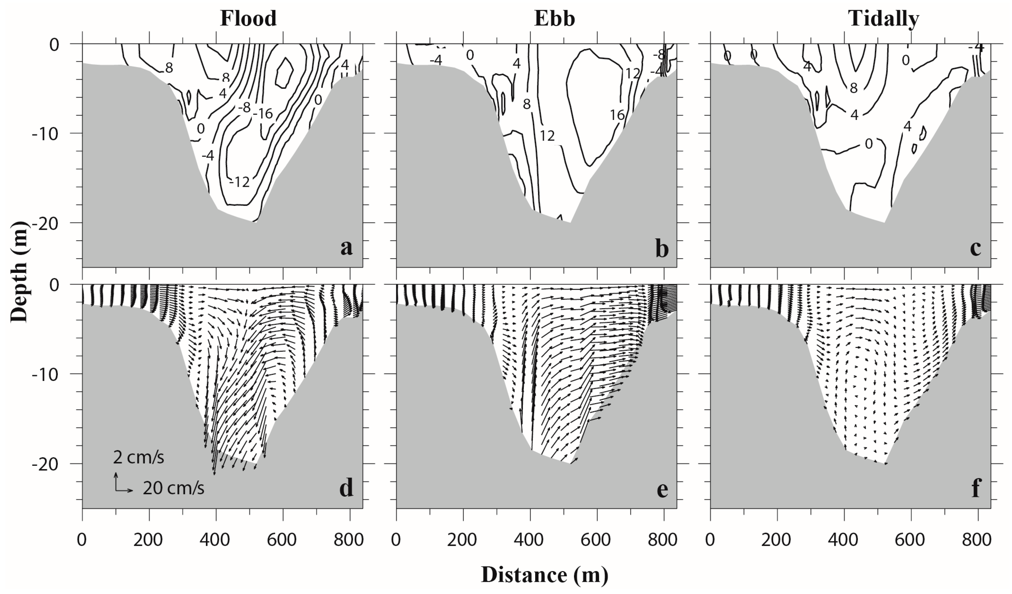
3.5. Residual Currents in the Barataria Pass over One Tidal Cycle

Tidal, ebb-, and flood- averaged along-channel velocities for the same 25.6 h time period are shown in Figure 7. The location of the transect is shown in Figure 1b and the western shoal is on the left side of Figure 7. The magnitude of cross-sectionally averaged ebb tides is −0.46 m/s, and that of cross-sectionally averaged flood tides is 0.33 m/s. The transverse structure of the along-channel residual current differs significantly between ebb and flood tides. For ebb tide, the maximum outflow is at the surface near the western shoal, inclining against the western bank of the deep channel. For flood tide, the maximum inflow is near the mid-depth in the central deep channel. Vertical velocity shear is much larger along the eastern bank than along the western bank. The magnitude of spatially averaged residual current during the 25.6 h period is −0.09 m/s, which is in the ebb direction. The maximum residual current is near the western shoal with the magnitude close to −0.3 m/s.
Using idealized numerical experiments, Cheng and Valle-Levinson [35] studied the sensitivity of estuarine exchange flow pattern on two nondimensional parameters, the Rossby number R 0 ( U / f B , where U is the estuarine circulation velocity, f is the Coriolis parameter, and B is the width of the channel) and the Ekman number E k ( A z / f H 2 , where A z is the vertical eddy viscosity, H is water depth, and f is the Coriolis parameter). They demonstrated that the exchange flow is vertically sheared at large R 0 , and horizontally sheared at large E k . In our case ( R 0 1.72 ,   E k 2.06 ), the residual current is both vertically and horizontally sheared, which is similar to their case shown in Figure 5c ( R 0 = 2.63 ,   E k = 1 ) of [35]. For a triangular shaped cross section, Wong [36] showed that the estuarine circulation is outward at the surface and inward at the bottom of the deep channel due to the interaction between baroclinic force and triangular bathymetry. Field observations at Barataria Pass captured this characteristics [31], in which the inflow is very weak. Our model also reproduces a weak inflow near the bottom of the eastern slope (Figure 7c). The asymmetry of estuarine–ocean exchange, i.e., inflow tending to the right side of the channel and outflow to the left side (when looking up-estuary) may be attributed to the Coriolis force [37].
The transverse structure of cross-channel residual current also differs significantly between ebb and flood tides. The maximum flood-averaged and ebb-averaged velocity can reach 0.2 m/s and 0.16 m/s, respectively. The ebb-averaged velocity exhibits no horizontal divergence or convergence in the deep channel (Figure 8b,e), while the flood-averaged velocity shows a strong convergence close to the surface in the mid-channel (Figure 8a,d). However, no closed cell circulation exists for the flood average (Figure 8d), which is different from that described in Nunes and Simpson [1]. The tidally averaged cross-channel velocity is relatively weaker (Figure 8c), and it displays a clockwise circulation cell in the western channel and an even weaker counterclockwise cell in the eastern channel (Figure 8f).

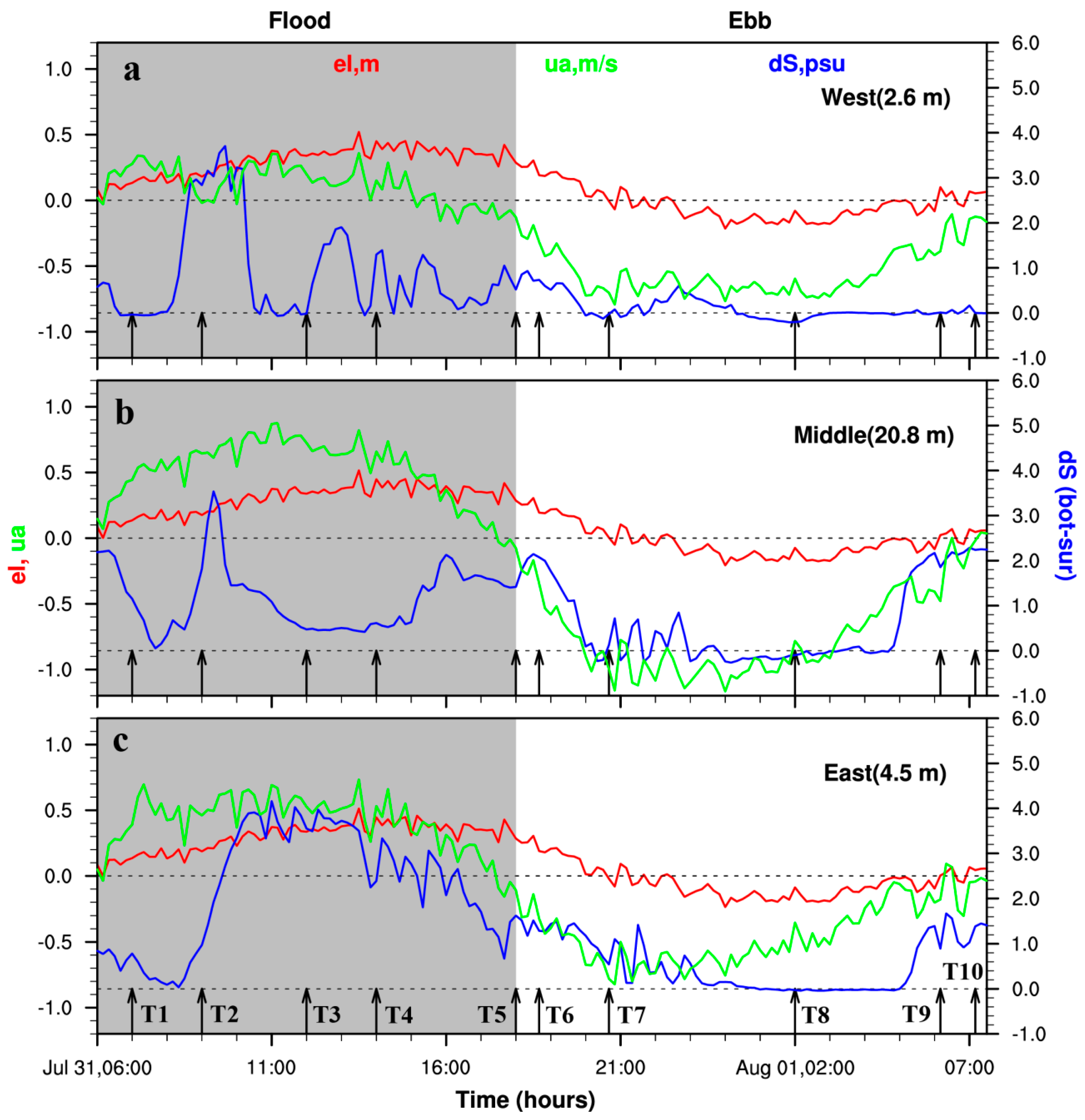
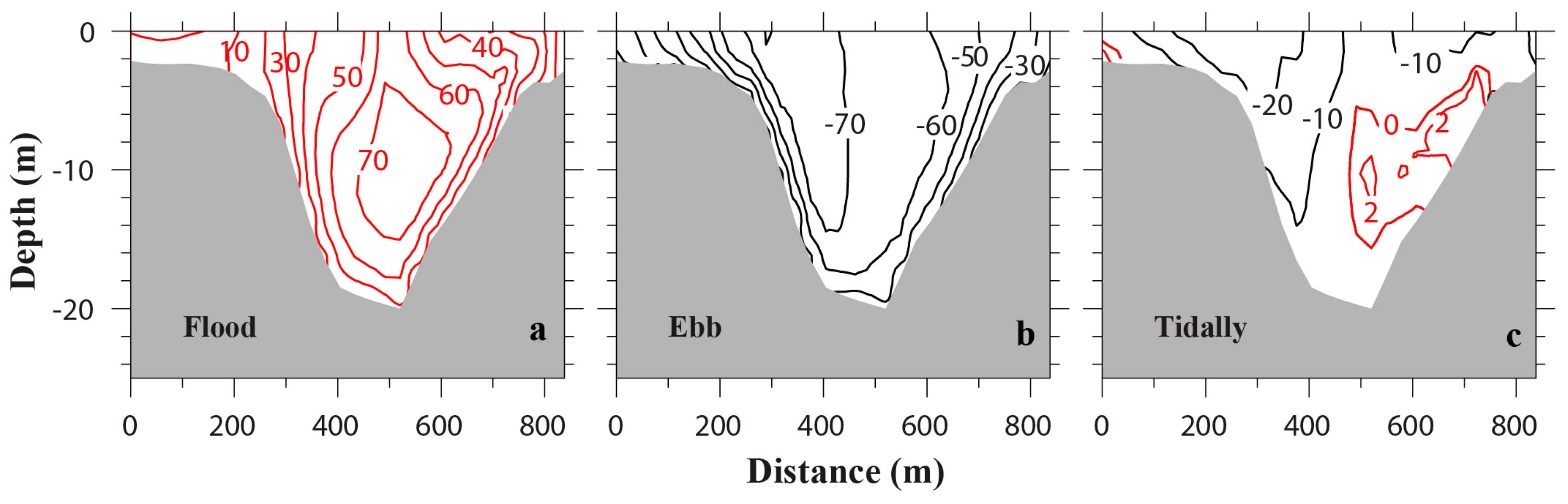
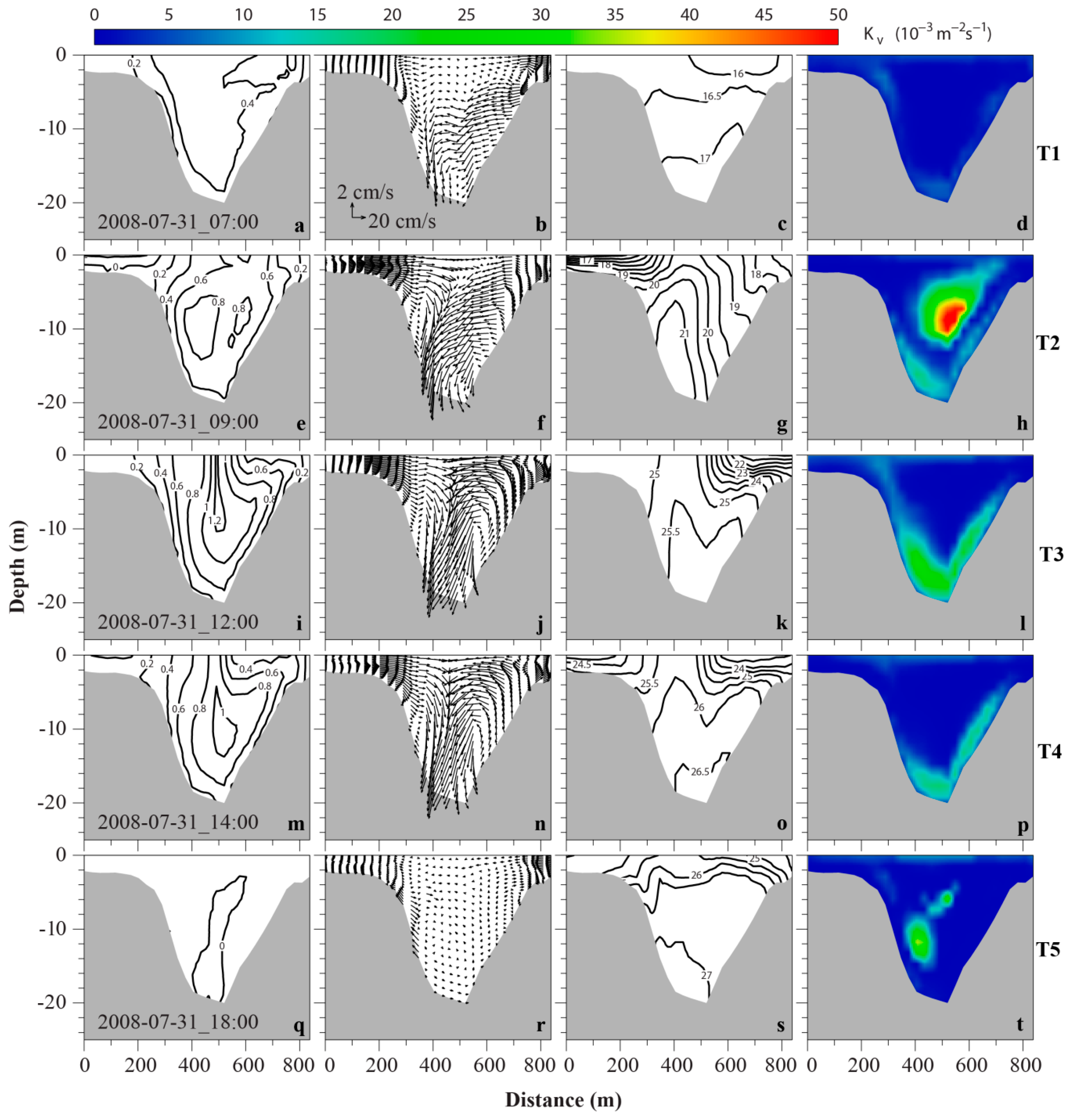
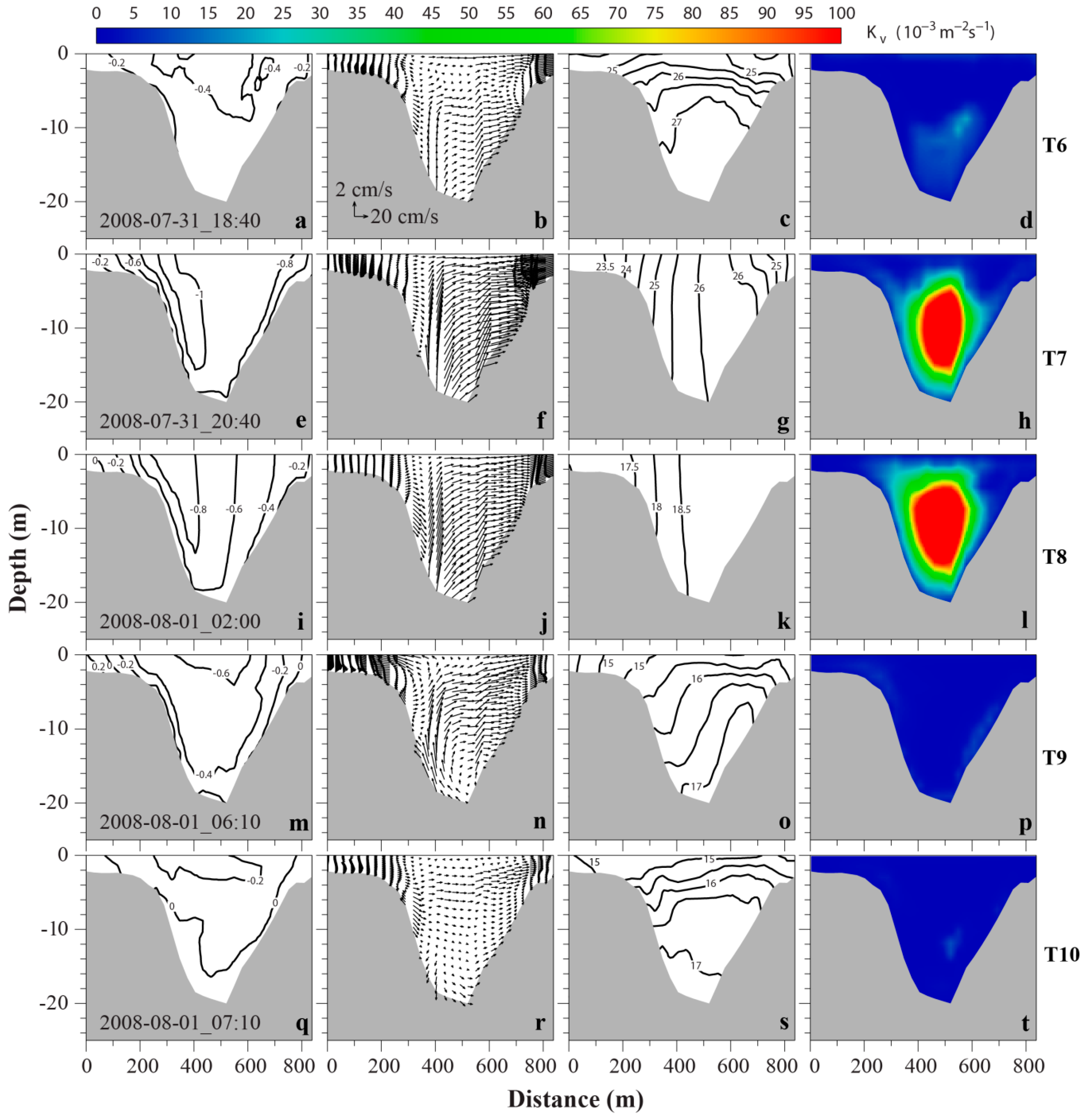
3.6. Time Series of Cross-Sectional Salinity and Currents Structures

Figure 9 shows the temporal evolution of along-channel velocity, lateral circulation, salinity, and turbulent vertical eddy viscosity for the Barataria Pass transect during flood tide. Each row represents a time instance indicated by an arrow in Figure 6. One hour after the flood starts (T1 in Figure 6), stratification is weak (bottom-top salinity difference ~1) across the deep channel and eastern shoal, and the western shoal is almost well-mixed (Figure 9c). Strong lateral circulation mainly occurs in the mid-depth with a convergence zone below 10 m in the deep channel (Figure 9b). The along-channel velocity is ~0.4 m/s, extending almost the whole deep channel. Thus, vertical and lateral velocity shear is weak. The vertical eddy viscosity is mostly smaller than 0.005 m2/s, probably due to the small flood current magnitude and its shears.
Two hours later (T2 in Figure 6), the whole water column becomes more or less well-mixed across the deep channel and eastern shoal, while in the western shoal a sharp salinity stratification develops with bottom-top salinity difference ~3 in 2 m water column (Figure 9g). The distribution of salinity, and thus density, in the cross-channel direction is such that lateral baroclinic pressure gradients are directed from the central part of the deep channel towards the shoals. This is similar to the situation pointed out in Nunes and Simpson [1]. Based on their theory, such pressure gradient force will induce a lateral circulation with convergence at the surface and divergence near the bottom. This indeed occurs in our numerical results. Surface lateral flow at the west half of the channel changes from ~0.1 m/s westward to ~0.2 m/s eastward between T1 and T2. A pair of counter-rotating circulations can be clearly seen at T2 with strong convergence 2 m below the surface. Contrast to the idealized case in Lerczak and Geyer [2], the two circulation cells are not closed at this time. The maximum along-channel tidal velocity reaches ~0.8 m/s, confined at the mid-depth of the central channel (Figure 9e). The vertical shear in along-channel velocity is relatively weak, while the horizontal shear is great, which is, over the western slope, ~0.6 m/s within 200 m distance. It follows that Nunes and Simpson’s argument is also applicable here in that differential advection of along-channel current is at least one of the mechanisms to generate the lateral salinity gradient. Strong vertical mixing (maximum eddy viscosity ~0.05 m2/s, Figure 9h) occurs at the mid-depth and bottom boundary layer, where either tidal currents or bottom friction are strong (Figure 9e). Strong turbulence mixing tends to destratify the water column, which explains the relatively uniform salinity distribution in the deep channel and east shoal (Figure 9g).
At the maximum flood (T3), the along-channel velocities intensify. Maximum along-channel velocity, located at channel thalweg, reaches ~1.2 m/s and extends to the surface (Figure 9i), which is quite different from T2 (Figure 9e). The lateral shear of along-channel velocity, i.e., differential advection, is 1.0 m/s across 300 m distance on both sides. However, salinity distribution changes drastically. The western shoal is completely well-mixed at this time, while the eastern shoal and part of the east channel have surface stratification with a salinity difference of ~3 within 5–6 m depth (Figure 9k). The stratification in the deep channel, especially below 10 m, is weak, because the tidal mixing is relatively high (vertical eddy viscosity ~0.03 m2/s) at the bottom boundary (Figure 9l). The lateral circulation pattern is similar to that at T2, but with intensified strength. The convergent zone rises to the ocean surface and the right circulation cell is now a complete circle (Figure 9j).
Four hours before the end of flood (T4), differential advection still persists, although the maximum along-channel tidal current has reduced to ~1 m/s and lowered below the surface (Figure 9m). Turbulence mixing weakens (Figure 9p). Hence, a weak stratification (bottom–surface salinity difference ~1.5) develops at the western shoal (Figure 9o). The salinity distribution shows a more symmetric pattern relative to the axis of the channel compared with T1, T2, and T3. As a result, the counter-rotating lateral circulation cells are more symmetric and fully developed (Figure 9n).
At the flood slack (T5), the surface water column becomes stratified in the upper 6 m (salinity difference ~1) while the deep channel is almost well-mixed (Figure 9s). The lateral circulation almost completely disappears in the deep channel (Figure 9r).
At the beginning of ebb tide (T6), although the along-channel ebb current increases to ~0.4 m/s (Figure 10a), the salinity distribution and vertical stratification (Figure 10c) are almost the same as that of T5. There is a weak (less than 0.1 m/s) eastward lateral flow below 6 m (Figure 10b).
Two hours later (T7), the along-channel ebb current reaches above 1.0 m/s, locating mostly on the western slope and reaching the sea surface. The magnitude of along-channel velocity across the majority of the cross section is ~0.8 m/s (Figure 10e), which induces large tidal mixing (maximum vertical eddy viscosity ~0.16 m2/s, Figure 10h). Thus, the whole water column is vertically well-mixed (Figure 10g). However, a horizontal salinity gradient exists, with higher salinity located near the channel axis, fresher water on both shoals. The western shoal is fresher than the eastern shoal (Figure 10g). This is because freshwater is flushed out of the estuary through the western shoal, as shown in Figure 7b,c. The lateral circulation shows mostly eastward currents in the deep channel across the whole water column, while the eastern shoal has a convergence area (Figure 10f).
During the next five hours, this cross section is always vertically well-mixed and salinity decreases constantly due to freshwater outflow. The turbulence mixing remains intense in the deep channel during this period. The maximum vertical eddy viscosity can reach up to 0.2 m2/s, which results in the water column in the east half of the channel vertically and horizontally well-mixed (Figure 10k, T8). The water column in the west half of the channel is also vertically well-mixed, but has a weak (~1) horizontal salinity decrease westward. The structure of lateral circulation and along-channel velocity remains the same, although the maximum ebb velocity has decreased from 1.0 m/s at T7 to 0.8 m/s at T8.
Later during the ebb period (T9), the vertical stratification returns (Figure 10o), probably due to greatly reduced turbulence vertical eddy viscosity (Figure 10p). The vertical salinity difference is ~2 in the deep channel and on the eastern shoal. Lateral circulation shows a weak flow divergence close to the surface near the western slope (Figure 10n). The maximum along-channel ebb current moves to the surface central channel and its magnitude decreases to 0.6 m/s (Figure 10m).
At the ebb slack (T10), salinity distribution go back to similar to T1 situation. The western shoal is almost vertically uniform. Strong stratification (salinity difference ~2 over 6 m depth) occurs in the upper water column of the deep channel and on the eastern shoal. The lower water column in the deep channel has a weak stratification (Figure 10s). Lateral circulation is greatly reduced compared to other time instances of the ebb tide (Figure 10r).

4. Discussion

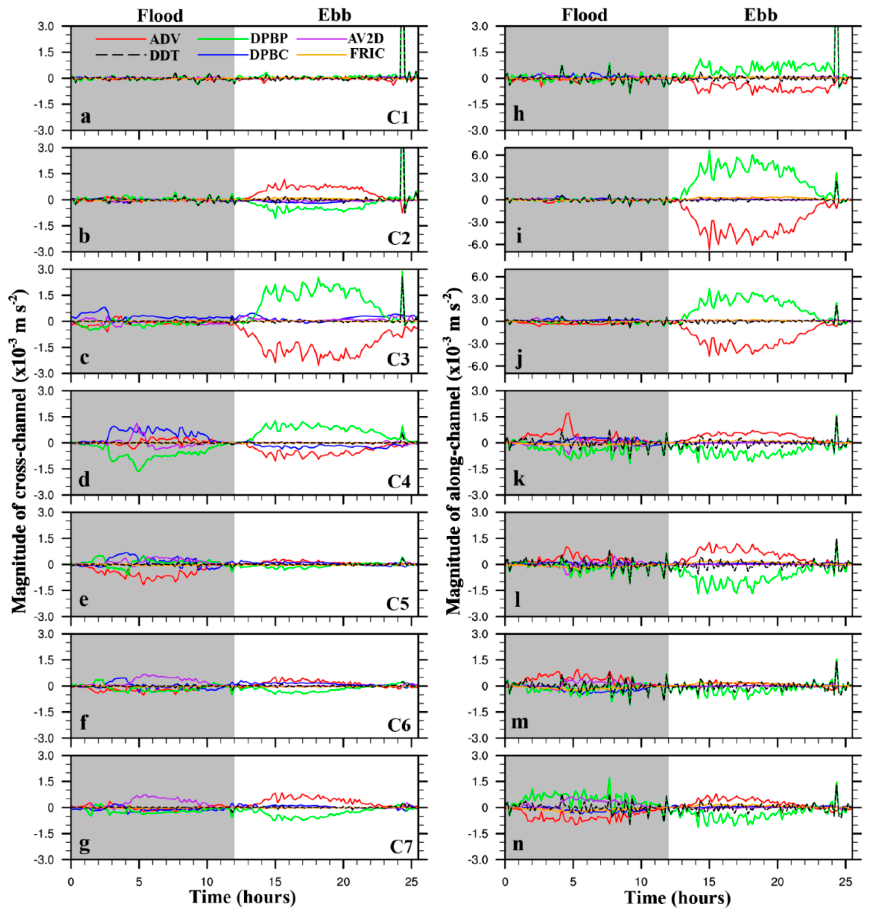
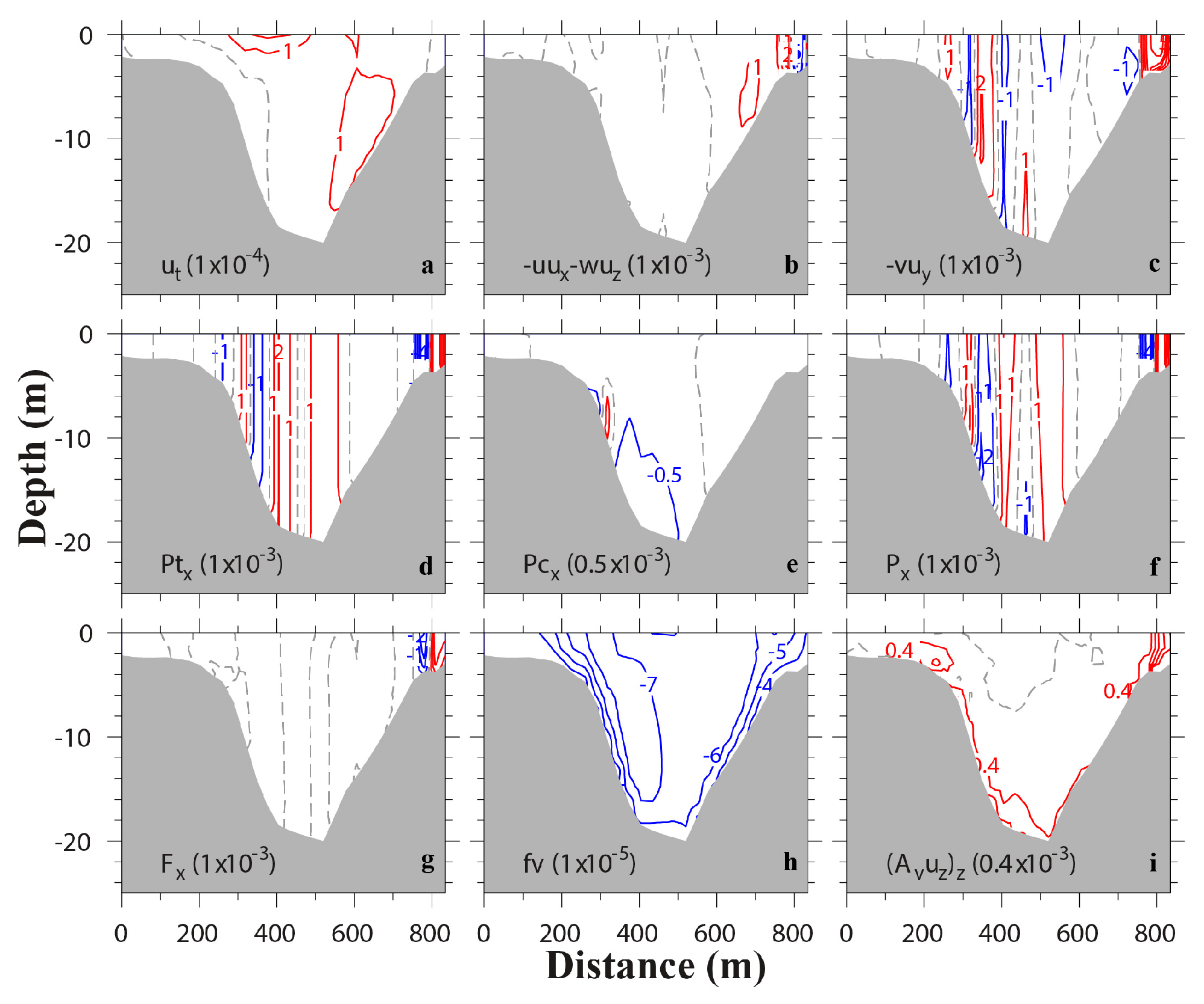
4.1. Depth-Averaged Momentum Balance

The Coriolis force, wind stress, and horizontal diffusion in Equations (1) and (2) are at least one order of magnitude smaller than the other terms during the 25.6 h period. Thus, these three terms are not shown. Figure 11 shows time series of six terms (DDT, ADV, DPBP, DPBC, FRIC, and AV2D) in Equations (1) and (2) at seven locations across the channel (Figure 1c). The momentum balance across this narrow channel is very complex, as various locations have different characteristics.
In the along-channel momentum balance, the dominant balance is between the barotropic pressure gradient and the nonlinear advection, especially during ebb tide. The magnitudes of these two terms for stations on the western side (C2 and C3, Figure 11i,j) of the channel are at least twice as greater as that of other stations. This is because maximum ebb currents flush out of the Barataria Bay near these two stations. The sign of barotropic pressure and nonlinear advection at stations on the west channel (C1–C3, Figure 11h–j) is opposite to those on the east channel (C4–C7, Figure 11k–n). There is a spike during ebb tide, similar to that in Huang et al. [33]. The reason for this spike is not clear. During flood tide, the magnitudes of all terms at stations in the western channel (C1–C3, Figure 11h–j) are relatively small. This is because the sign of terms in the upper layer is opposite to that of the lower layer during flood tide. They offset each other after integrating over depth. The balance is among the DDT, nonlinear advection, barotropic pressure gradient, baroclinic pressure gradient, and the AV2D.
In the cross-channel momentum balance, the characteristics are similar to that of along-channel, i.e., the dominant balance is between advection term and the barotropic pressure gradient. Excluding station C1, the signs of advection and barotropic pressure terms at the westmost station (C2, Figure 11b) and the eastmost station (C7, Figure 11g) are the same, but opposite to the stations of the deep channel (C3, C4, Figure 11c,d). During flood tides, the balance is among the DDT, nonlinear advection, barotropic pressure gradient, baroclinic pressure gradient, and the AV2D. Note that, the baroclinic pressure is great at stations in the deep channel, and the magnitude is larger than that of along-channel. This indicates the lateral salinity gradient play an important role in momentum balance.

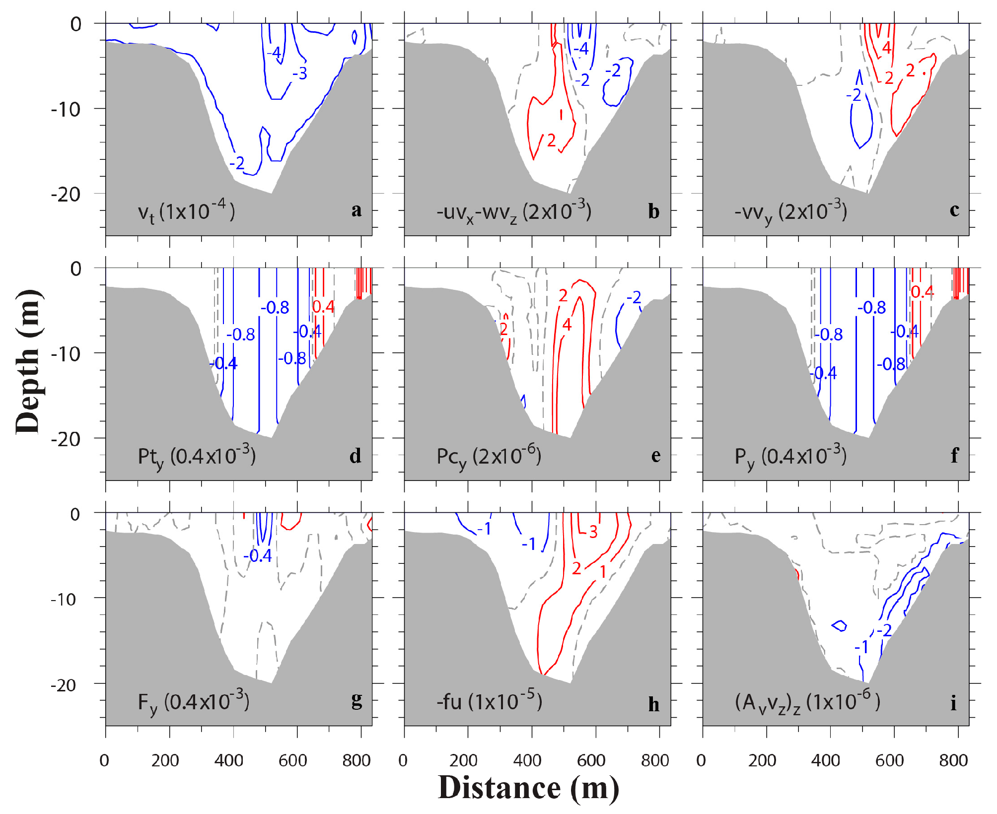
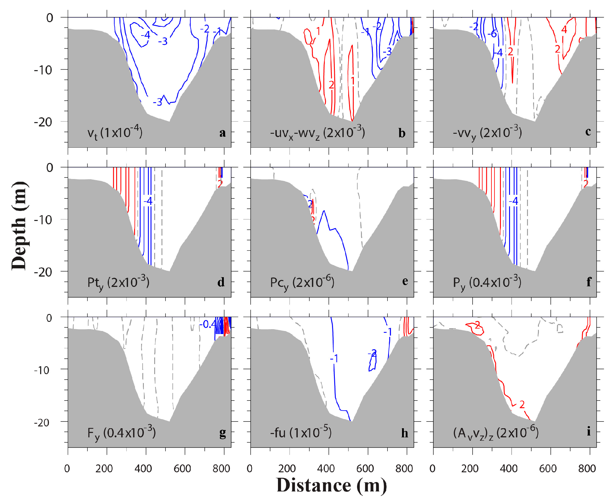
4.2. Driving Mechanism of Lateral Circulation

Lerczak and Geyer [2] pointed out that lateral advection plays an important role in the estuarine dynamics when lateral flows are strong enough to advect water parcels relative to 0.5 times the breadth of the channel ( 4 | v | / σ B 1 , where | v | is the absolute value of lateral velocity amplitude, σ is the semidiurnal tidal frequency, and B is the channel width) in a tidal cycle. As shown in previous results, lateral circulation in the Barataria Pass is strong both during maximum flood and maximum ebb. Thus, lateral advection is expected to be an important term in the momentum balance. The 3-D momentum Equations (3) and (4) are used to explore the generation mechanisms of the lateral circulation.
Transverse distributions of various momentum terms of along- and cross-channel components at T3 (flood tide) are shown in Figure 12 and Figure 13, respectively. In the along-channel momentum equation, baroclinic pressure gradient (Figure 12e), Coriolis force (Figure 12h) and vertical stress divergence (Figure 12i) are at least two orders of magnitude less than other terms at this time, thus are less important. The total pressure gradient comes from the barotropic pressure gradient (Figure 12d), and the largest terms are the nonlinear advection terms (Figure 12b,c). Lateral advection of along-channel momentum (Figure 12b, u v x w v z ) is one of the largest terms in the momentum balance. This term has a similar pattern but opposite sign with the along-channel momentum advection ( v v y ). The main force balance at this time is between non-linear advection and the barotropic pressure gradient, which is consistent with the result in 2-D momentum analysis.
In the cross-channel momentum balance, Coriolis force (Figure 13h), although small, has exactly the same pattern as the transverse distribution of along-channel velocity (Figure 9i). Differential advection of the flood current at this time is clearly shown in the picture. The baroclinic pressure gradient (Figure 13e) has almost the same magnitude as the barotropic pressure gradient (Figure 13d), especially near the bottom, due to its magnitude increasing with depth. The baroclinic pressure gradient is mostly positive in the whole channel, except near the eastern shoal. Combining with the salinity distribution at the transect (Figure 9k), it indicates that the conceptual model of cross-channel baroclinic pressure gradient induced by differential advection is applicable here. However, the simple diagnostic model proposed by Nunes and Simpson [1] to explain the mechanism of lateral circulation generation, in which the momentum balance is between cross-channel pressure gradient and vertical stress divergence, seems to be oversimplified. Our numerical experiment shows that vertical stress divergence is mostly confined to the near bottom layer of the eastern slope (Figure 13i). Several other terms—nonlinear advection (Figure 13b,c) and horizontal stress divergence (Figure 13g)—are as important as the terms suggested in [1].
During ebb tide (i.e., at T7), the main momentum balance in the along-channel direction is among the nonlinear advection terms and the barotropic pressure gradient (Figure 14), which is the same as during the flood tide (Figure 12).
In the cross-channel momentum balance, the barotropic pressure gradient (Figure 15d) dominates the baroclinic pressure gradient (Figure 15e). Thus, contour lines of the total cross-channel pressure gradient (Figure 15f) are very similar to that of the former. It seems that at this time the main momentum balance is between along-channel advection of cross-channel momentum (Figure 15c) and pressure gradient (Figure 15f) over most of the cross-section area, both of which have alternative positive and negative vertical stripes and, when added together, almost cancel out each other. At the eastern shoal, all terms, excluding Coriolis force (Figure 15h) and baroclinic pressure gradient (Figure 15e), are needed in order to balance the cross-channel momentum equation. Because of the insignificant contribution from the baroclinic pressure gradient, no obvious convergence or divergence occurs in this transect during the ebb period (Figure 10, second column). This is in clear contrast to the near surface convergence that happens during flood tide (Figure 9, second column).

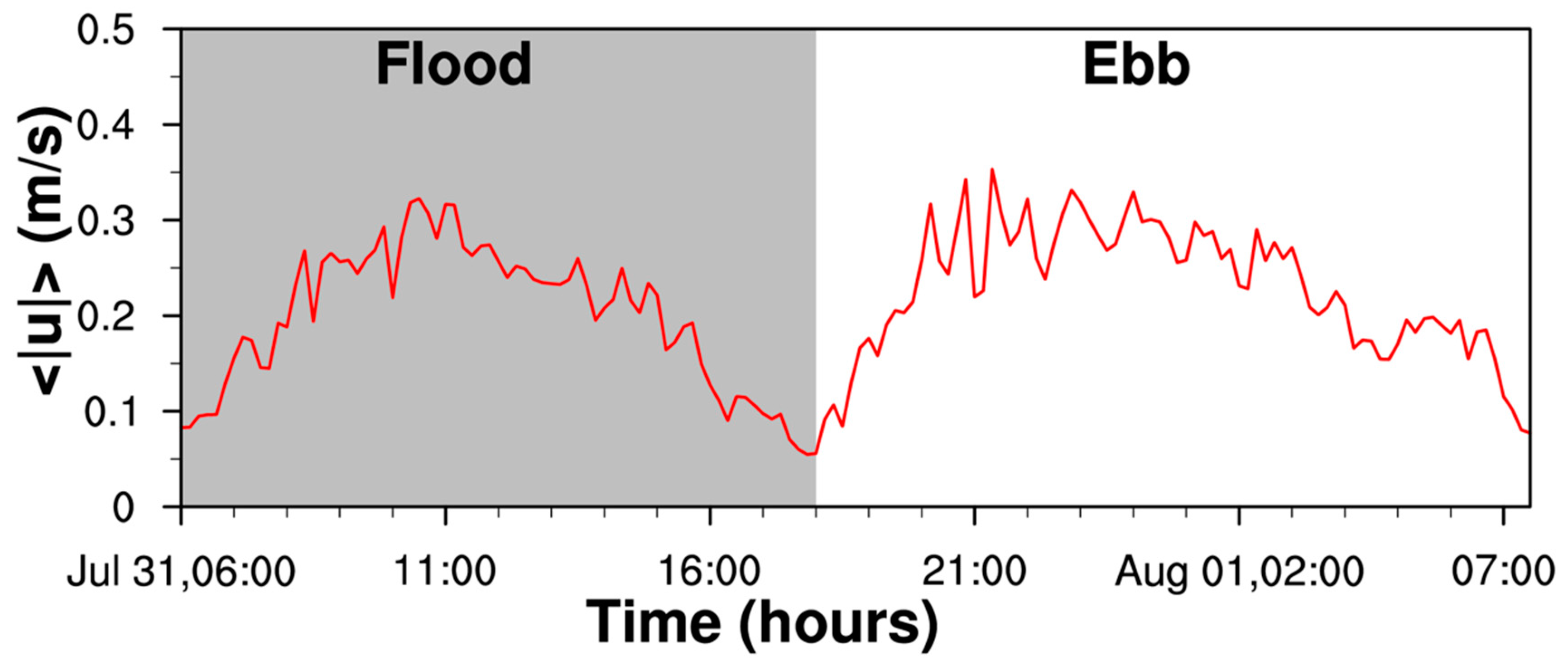
4.3. Flood–Ebb Asymmetry

Here, we follow Lerczak and Geyer [2] using the cross-channel average of depth-averaged velocity amplitude < | u | > = 1 A | u | d A ( | u | is the absolute value of depth-averaged cross-channel velocity, A is the cross-channel area) to represent the strength of the lateral flow. The result is shown in Figure 16. The maximum < | u | > during flood is 0.32 m/s, while the maximum during ebb is 0.34 m/s. Generally, cross-channel current amplitude during ebb is comparable, even slightly greater than that during flood, which is different from the idealized case [2], in which lateral circulation is about four times stronger during flood tides than during ebb tides. However, this inconsistence is also observed in James River estuary [14], where the lateral circulation shows no flood–ebb asymmetry during spring tides, and a reversed asymmetry during neap tides, that is stronger during ebb than during flood. Li et al. [14] attribute negligible flood–ebb variations during spring tides to turbulent mixing, which in their numerical experiment was simulated via a turbulence closure model. It reduces the vertical shear and the flood–ebb asymmetry in the vorticity generation. In comparison, the idealized case of Lerczak and Geyer [2] used a constant eddy viscosity. In our numerical experiment, turbulent mixing is simulated using the Mellor-Yamada 2.5 turbulence closure model and the 25.6 h diurnal tidal cycle is close to tropic tide. Maximum turbulent vertical viscosity is twice as great during ebb (Figure 10, last column) as during flood (Figure 9, last column). Therefore, our simulation result is more similar to Li et al. [14] than to Lerczak and Geyer [2].
During flood tide, lateral circulation shows asymmetry across the section (Figure 9f,j,n). The counterclockwise circulation on the east side is stronger, which is due to the presence of lower salinity water close to and over the eastern shoal (Figure 9k,o). This fresher water increases the lateral baroclinic pressure gradient on the east side, and thus enhances the strength of the lateral circulation cell at this side. The low salinity water is from the Mississippi River plume based on analyses of in-situ observational data and numerical simulation result [22].
Another asymmetry between flood and ebb tides lies in that maximum flood currents are always located, more or less, at the central part of the deep channel (Figure 9, first column), while maximum ebb currents, when they are greater than 0.8 m/s, are located closer to the western shoal or over the western slope (Figure 10e,i). Only when maximum ebb currents are below 0.6 m/s, they move back to the middle of the channel (Figure 10a,m,q).

5. Conclusions

Barataria Pass is a tidal inlet that connects the Barataria Bay to the continental shelf. Previous investigation has introduced the tidal straining effect on density stratification during the same 25.6 h period along the same transect [22]. In this study, we conduct a numerical model simulation and illustrate that the lateral variations in the salinity and velocity fields are comparable to or even larger than the vertical variations within a diurnal tidal cycle.
The density distribution within any estuary is a result of both advective and mixing processes. In Barataria Pass, the turbulent mixing is closely related to the magnitude of ebb/flood current and the strength of the tidal bottom boundary layer. Characteristics of horizontal advection processes in the inlet are that maximum flood currents are located at the central part of the deep channel for a large part of the flood period. This differential advection [1], when acting upon the along-channel density gradient, produces a distinct density difference between the shoal and channel waters. In addition, the advection of Mississippi River water to the eastern channel during part of the flood period further enhances the density difference. On the contrary, maximum ebb currents swing between the western slope and central surface of the channel during the ebb. When maximum ebb flows are at the western slope, the differential advection mechanism does not work. When they go back to the channel center, the salinity contour lines are mostly horizontal due to weak vertical turbulence mixing. Thus, both situations are not favorable to produce an extreme density near the middle of the channel.
During flood period, when density distribution is high near the channel center and low at both shoals, the horizontal pressure gradient drives a lateral circulation with two counter-rotating cells and surface or near surface convergence. This result from the Barataria Pass is similar to that reported by Nunes and Simpson [1]. However, detailed analysis of momentum equations indicates that, in addition to the pressure gradient and vertical stress divergence, nonlinear advection and horizontal stress divergence are also important terms.
During ebb period, the lateral circulation is mostly eastward for the whole water column and persisting for almost the whole period. The surface divergence suggested by the differential advection mechanism is either non-existent or lasting for a very short period. The main momentum balance across most of the transect is between the along-channel advection of cross-channel momentum and pressure gradient. In addition, the sectional averaged lateral velocity magnitude during ebb is comparable to that during flood, which is different from the idealized numerical experiment [2].
Interactions among lateral circulation, along-channel tidal currents, and density stratification are complex processes. Lateral circulation can play a critical role in the dynamics of estuaries. It can act as a driving term for the estuarine exchange flow [2], and thus alter the along-channel momentum budget [38]. During flood tide, lateral circulation transported near-bed sediment out of the channel toward the shoal [37]. During ebb tide, it created a convergence in suspended sediment at the transition between channel and shoal [39]. Trapping by lateral circulation alters the lateral distribution of bed sediment. The idealized numerical experiment with constant eddy coefficients [2] demonstrated that the lateral circulation can be significantly different over a spring-neap cycle and density stratification can inhibit lateral circulation. Our study can be a starting point for further investigations of interactions among lateral circulation, estuarine circulation, and estuarine stratification in the partially stratified tidal inlet, the Barataria Pass.

Supplementary Materials

FVCOM simulation data are publicly available through the Gulf of Mexico Research Initiative Information and Data Cooperative (GRIIDC) at https://data.gulfresearchinitiative.org (DOI: 10.7266/n7-1qe9-mg27).

Author Contributions

Conceptualization, L.C. and H.H.; Investigation, L.C., H.H., C.L.; Writing-Original Draft Preparation, L.C.; Writing-Review & Editing, H.H., C.L., D.J.; Visualization, L.C.; Funding Acquisition, D.J., H.H.

Funding

This research was made possible in part by a grant from The Gulf of Mexico Research Initiative. L.C. was also funded by the Economic Development Assistantship from the Graduate School, Louisiana State University.

Acknowledgments

Portions of this research were conducted with high performance computational resources provided by Louisiana State University (http://www.hpc.lsu.edu) and the Louisiana Optical Network Initiative (http://www.loni.org).

Conflicts of Interest

The authors declare no conflict of interest.

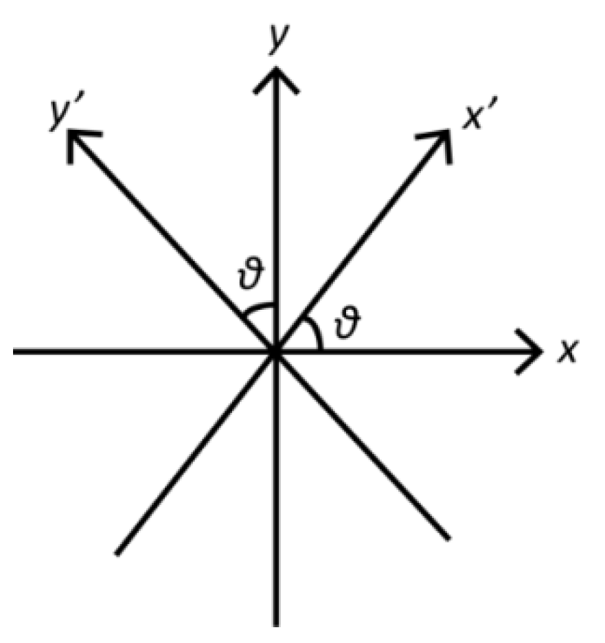
Appendix A. Decomposition of Vectors into Along- and Cross-Channel Directions

In x - y - σ coordinates, where x -direction is defined to the east and y -direction to the north, the FVCOM x - and y -axis 3-D momentum equations are written as:
u D t D U D T = u 2 D x A D V U X u v D y A D V V X u ω σ A D V W X + f v D C O R X g D ζ x D P B P X g D ρ 0 [ x ( D σ 0 d σ + σ ρ D x ) ] D P B C X + 1 D σ ( K m u σ ) V V I S C X + F x H V I S C X
v D t D V D T = u v D x A D V U Y v 2 D y A D V V Y v ω σ A D V W Y f u D C O R Y g D ζ y D P B P Y g D ρ 0 [ y ( D σ 0 d σ + σ ρ D y ) ] D P B C Y + 1 D σ ( K m v σ ) V V I S C Y + F y H V I S C Y
where ( u , v ) are the velocity components in the ( x , y ) directions, σ is the vertical coordinate.
In order to quantify along- and cross-channel momentum balance, we choose the along-channel direction ( y ) to be aligned with the channel. It is positive when pointing into the estuary. The cross-channel direction ( x ) is defined to be positive when pointing to the eastern boundary (Figure A1). The relationship between ( u , v ) and ( u , v ) , ( x , y ) and ( x , y ) are as following:
u = u c o s θ + v s i n θ
v = u s i n θ + v c o s θ
x = ( x x 0 ) c o s θ + ( y y 0 ) s i n θ
y = ( x x 0 ) s i n θ + ( y y 0 ) c o s θ
where θ is the angle between the x -direction (cross-channel) and the x -direction.
Figure A1. Illustration of x-y coordinate transformed to x’-y’ coordinate.
Jmse 06 00159 g0a1
In x - y coordinates, the momentum equations are written as:
u D t D U D T = u 2 D x A D V U X u v D y A D V V X u ω σ A D V W X + f v D C O R X g D ζ x D P B P X g D ρ 0 [ x ( D σ 0 d σ + σ ρ D x ) ] D P B C X + 1 D σ ( K m u σ ) V V I S C X + F x H V I S C X
v D t D V D T = u v D x A D V U Y v 2 D y A D V V Y v ω σ A D V W Y f u D C O R Y g D ζ y D P B P Y g D ρ 0 [ y ( D σ 0 d σ + σ ρ D y ) ] D P B C Y + 1 D σ ( K m v σ ) V V I S C Y + F y H V I S C Y
To project the momentum equations into the cross- and along-channel directions, we treat each term in the momentum equations as a vector in the ( x , y ) direction and then apply the same decomposition as Equations (A3) and (A4). Thus terms in x - y coordinates can be calculated by corresponding terms in x - y coordinates as follows:
D U D T = u D t = ( u c o s θ + v s i n θ ) D t = u D t c o s θ + v D t s i n θ = D U D T c o s θ + D V D T s i n θ
D V D T = v D t = ( u s i n θ + u c o s θ ) D t = u D t s i n θ + v D t c o s θ = D U D T s i n θ + D V D T c o s θ
Terms ADVUX’+ADVVX’, ADVUY’+ADVVY’, ADVWX’, ADVWY’, CORX’, CORY’, DPBPX’, DPBPY’, DPBCX’, DPBCY’, VVISCX’, VVISCY’, HVISCX’, and HVISCY’ can be calculated with the same method. While ADVUX’, ADVVX’, ADVUY’, and ADVVY’ should be calculated by the finite volume difference. For example, ADVUX’ can be calculated as:
u 2 D x d x d y = u u D d y = U I J × ( U I J 1 U I J 2 ) × D I J × d y
where U I J , U I J 1 and U I J 2 are shown in Figure A2.
Figure A2. Illustration of local coordinate used to calculate the horizontal advection terms.
Jmse 06 00159 g0a2
With Equations (A3)–(A6), we have:
d y = s i n θ + c o s θ d y
U I J = U I J c o s θ + V I J s i n θ
U I J 2 1 = U I J 2 1 × c o s θ + V I J 2 1 × s i n θ
Substituting Equations (A10)–(A12) into Equation (A9),
A D V U X = u 2 D y = u 2 D y s i n θ c o s 2 θ + u v D y s i n 2 θ c o s θ + v u D y s i n 2 θ c o s θ + v 2 D y s i n 3 θ + u 2 D x c o s 3 θ + u v D x s i n θ c o s 2 θ + v u D x s i n θ c o s 2 θ + v 2 D x s i n 2 θ c o s θ
With the same method, A D V V X ,   A D V U Y , and A D V V Y are given as:
A D V V X = u v D y = u 2 D y s i n θ c o s 2 θ u v D y s i n 2 θ c o s θ + v u D y c o s 3 θ + v 2 D y s i n θ c o s 2 θ + u 2 D x s i n 2 θ c o s θ + u v D x s i n 3 θ v u D x s i n θ c o s 2 θ v 2 D x s i n 2 θ c o s θ
A D V U Y = u v D x = u 2 D y s i n 2 θ c o s θ + u v D y s i n θ c o s 2 θ v u D y s i n 3 θ + v 2 D y s i n 2 θ c o s θ u 2 D x s i n θ c o s 2 θ + u v D x c o s 3 θ v u D x s i n 2 θ c o s θ + v 2 D x s i n θ c o s 2 θ
A D V V Y = v 2 D y = u 2 D y s i n 2 θ c o s θ u v D y s i n θ c o s 2 θ v u D y s i n θ c o s 2 θ + v 2 D y c o s 3 θ u 2 D x s i n 3 θ + u v D x s i n 2 θ c o s θ + v u D x s i n 2 θ c o s θ v 2 D x s i n θ c o s 2 θ

References

  1. Nunes, R.A.; Simpson, J.H. Axial convergence in a well-mixed estuary. Estuar. Coast. Shelf Sci. 1985, 20, 637–649. [Google Scholar] [CrossRef]
  2. Lerczak, A.J.; Geyer, W.R. Modeling the lateral circulation in straight, stratified estuaries. J. Phys. Oceanogr. 2004, 34, 1410–1428. [Google Scholar] [CrossRef]
  3. Li, C. Axial convergence fronts in a barotropic tidal inlet—Sand shoal inlet, VA. Cont. Shelf Res. 2002, 22, 2633–2653. [Google Scholar] [CrossRef]
  4. Li, C.; Valle-Levinson, A. A two-dimensional analytic tidal model for a narrow estuary of arbitrary lateral depth variation: The intratidal motion. J. Geophys. Res. Oceans 1999, 104, 23525–23543. [Google Scholar] [CrossRef] [Green Version]
  5. Valle-Levinson, A.; Li, C.; Wong, K.-C.; Lwiza Kamazima, M.M. Convergence of lateral flow along a coastal plain estuary. J. Geophys. Res. Oceans 2000, 105, 17045–17061. [Google Scholar] [CrossRef] [Green Version]
  6. Chant, R.J.; Wilson, R.E. Secondary circulation in a highly stratified estuary. J. Geophys. Res. Oceans 1997, 102, 23207–23215. [Google Scholar] [CrossRef] [Green Version]
  7. Lacy, J.R.; Monismith, S.G. Secondary currents in a curved, stratified, estuarine channel. J. Geophys. Res. Oceans 2001, 106, 31283–31302. [Google Scholar] [CrossRef] [Green Version]
  8. Pein, J.; Valle-Levinson, A.; Stanev, E.V. Secondary Circulation Asymmetry in a Meandering, Partially Stratified Estuary. J. Geophys. Res. Oceans 2018, 123, 1670–1683. [Google Scholar] [CrossRef]
  9. Li, C.; Chen, C.; Guadagnoli, D.; Georgiou Ioannis, Y. Geometry-induced residual eddies in estuaries with curved channels: Observations and modeling studies. J. Geophys. Res. Oceans 2008, 113, C01005. [Google Scholar] [CrossRef]
  10. Wargula, A.; Raubenheimer, B.; Elgar, S. Curvature- and Wind-Driven Cross-Channel Flows at an Unstratified Tidal Bend. J. Geophys. Res. Oceans 2018, 123, 3832–3843. [Google Scholar] [CrossRef]
  11. Chen, S.-N.; Sanford, L.P. Lateral circulation driven by boundary mixing and the associated transport of sediments in idealized partially mixed estuaries. Cont. Shelf Res. 2009, 29, 101–118. [Google Scholar] [CrossRef]
  12. Cheng, P.; Wilson, R.E.; Flood, R.D.; Chant, R.J.; Fugate, D.C. Modeling influence of stratification on lateral circulation in a stratified estuary. J. Phys. Oceanogr. 2009, 39, 2324–2337. [Google Scholar] [CrossRef]
  13. Scully, E.M.; Geyer, W.R.; Lerczak, A.J. The influence of lateral advection on the residual estuarine circulation: A numerical modeling study of the Hudson River Estuary. J. Phys. Oceanogr. 2009, 39, 107–124. [Google Scholar] [CrossRef]
  14. Li, M.; Liu, W.; Chant, R.; Valle-Levinson, A. Flood-ebb and spring-neap variations of lateral circulation in the James River estuary. Cont. Shelf Res. 2017, 148, 9–18. [Google Scholar] [CrossRef]
  15. Geyer, W.R. Three-dimensional tidal flow around headlands. J. Geophys. Res. Oceans 1993, 98, 955–966. [Google Scholar] [CrossRef]
  16. Vennell, R.; Old, C. High-resolution observations of the intensity of secondary circulation along a curved tidal channel. J. Geophys. Res. Oceans 2007, 112, C11008. [Google Scholar] [CrossRef]
  17. Lacy, J.R.; Stacey, M.T.; Burau, J.R.; Monismith, S.G. Interaction of lateral baroclinic forcing and turbulence in an estuary. J. Geophys. Res. Oceans 2003, 108, 3089. [Google Scholar] [CrossRef]
  18. Nidzieko, N.J.; Hench, J.L.; Monismith, S.G. Lateral circulation in well-mixed and stratified estuarine flows with curvature. J. Phys. Oceanogr. 2009, 39, 831–851. [Google Scholar] [CrossRef]
  19. Brocchini, M.; Calantoni, J.; Postacchini, M.; Sheremet, A.; Staples, T.; Smith, J.; Reed, A.H.; Braithwaite, E.F.; Lorenzoni, C.; Russo, A.; et al. Comparison between the wintertime and summertime dynamics of the Misa River estuary. Mar. Geol. 2017, 385, 27–40. [Google Scholar] [CrossRef]
  20. Hunt, S.; Bryan, K.R.; Mullarney, J.C. The influence of wind and waves on the existence of stable intertidal morphology in meso-tidal estuaries. Geomorphology 2015, 228, 158–174. [Google Scholar] [CrossRef]
  21. Van Maren, D.S.; Hoekstra, P. Seasonal variation of hydrodynamics and sediment dynamics in a shallow subtropical estuary: The Ba Lat River, Vietnam. Estuar. Coast. Shelf Sci. 2004, 60, 529–540. [Google Scholar] [CrossRef]
  22. Li, C.; Swenson, E.; Weeks, E.; White, J.R. Asymmetric tidal straining across an inlet: Lateral inversion and variability over a tidal cycle. Estuar. Coast. Shelf Sci. 2009, 85, 651–660. [Google Scholar] [CrossRef]
  23. Das, A.; Justic, D.; Inoue, M.; Hoda, A.; Huang, H.; Park, D. Impacts of mississippi river diversions on salinity gradients in a deltaic Louisiana estuary: Ecological and management implications. Estuar. Coast. Shelf Sci. 2012, 111, 17–26. [Google Scholar] [CrossRef]
  24. Marmer, H.A. The Currents in Barataria Bay; The Texas A.&M. Research Foundation Project 9; Texas A.&M.: College Station, TX, USA, 1948; p. 30. [Google Scholar]
  25. Snedden, G.A. River, Tidal, and Wind Interactions in a Deltaic Estuarine System. Ph.D. Thesis, Louisiana State University, Baton Rouge, LA, USA, 2006; p. 116. [Google Scholar]
  26. Chen, C.; Beardsley, R.C.; Cowles, G.; Qi, J.; Lai, Z.; Gao, G.; Stuebe, D.; Xu, Q.; Xue, P.; Ge, J.; et al. An Unstructured Grid, Finite-Volume Community Ocean Model FVCOM User Manual, 3rd ed.; Rep. 06-0602; SMAST/UMASSD: New Bedford, MA, USA, 2011. [Google Scholar]
  27. Chen, C.; Liu, H.; Beardsley, R.C. An unstructured grid, finite-volume, three-dimensional, primitive equations ocean model: Application to coastal ocean and estuaries. J. Atmos. Ocean. Technol. 2003, 20, 159. [Google Scholar] [CrossRef]
  28. Mellor, G.L.; Yamada, T. Development of a turbulence closure model for geophysical fluid problems. Rev. Geophys. 1982, 20, 851–875. [Google Scholar] [CrossRef]
  29. Galperin, B.; Kantha, L.H.; Hassid, S.; Rosati, A. A Quasi-equilibrium turbulent energy model for geophysical flows. J. Atmos. Sci. 1988, 45, 55–62. [Google Scholar] [CrossRef]
  30. Smagorinsky, J. General circulation experiments with the primitive equations. Mon. Weather Rev. 1963, 91, 99–164. [Google Scholar] [CrossRef]
  31. Li, C.; White, J.R.; Chen, C.; Lin, H.; Weeks, E.; Galvan, K.; Bargu, S. Summertime tidal flushing of Barataria Bay: Transports of water and suspended sediments. J. Geophys. Res. Oceans 2011, 116, C04009. [Google Scholar] [CrossRef]
  32. Walker, N.D.; Wiseman, W.J.; Rouse, L.J.; Babin, A. Effects of River Discharge, Wind Stress, and Slope Eddies on Circulation and the Satellite-Observed Structure of the Mississippi River Plume. J. Coast. Res. 2005, 21, 1228–1244. [Google Scholar] [CrossRef]
  33. Huang, H.; Justic, D.; Lane, R.R.; Day, J.W.; Cable, J.E. Hydrodynamic response of the Breton Sound estuary to pulsed Mississippi River inputs. Estuar. Coast. Shelf Sci. 2011, 95, 216–231. [Google Scholar] [CrossRef]
  34. Willmott, C.J. On the validation of models. Phys. Geogr. 1981, 2, 184–194. [Google Scholar] [CrossRef]
  35. Cheng, P.; Valle-Levinson, A. Influence of lateral advection on residual currents in microtidal estuaries. J. Phys. Oceanogr. 2009, 39, 3177–3190. [Google Scholar] [CrossRef]
  36. Wong, K.-C. On the nature of transverse variability in a coastal plain estuary. J. Geophys. Res. Oceans 1994, 99, 14209–14222. [Google Scholar] [CrossRef]
  37. Geyer, W.R.; Signell, R.P.; Kineke, G.C. Lateral trapping of sediment in partially mixed estuary. In Physics of Estuaries and Coastal Seas; AA Balkema: Brookfield, VT, USA, 1998; pp. 115–124. [Google Scholar]
  38. Geyer, W.R.; Trowbridge, J.H.; Bowen, M.M. The dynamics of a partially mixed estuary. J. Phys. Oceanogr. 2000, 30, 2035–2048. [Google Scholar] [CrossRef]
  39. Ralston, D.K.; Geyer, W.R.; Warner, J.C. Bathymetric controls on sediment transport in the Hudson River estuary: Lateral asymmetry and frontal trapping. J. Geophys. Res. 2012, 117, C10013. [Google Scholar] [CrossRef]
Figure 1. (a) Geographic location of the Barataria Estuary. S1–S6 are USGS stations. (b) Location of Barataria Pass. The coordinate is defined as positive x to the eastern bank, positive y to the upstream. The red line indicates the cross-section shown in (c) and is used in later analysis. (c) Cross-sectional view of Barataria Pass. The black lines indicate CTD measurements. C1–C7 are locations used for 2-D momentum equation analysis.
Jmse 06 00159 g001
Figure 2. Unstructured grid configured for the Finite Volume Coastal Ocean Model (FVCOM) Barataria Pass model: (a) whole computational domain; (b) local domain of Barataria Estuary; (c) local domain of Barataria Pass, with horizontal resolution ~50 m in the cross-channel direction and 30 m in the along-channel direction. Contours are interpolated bathymetry. White dash line indicates cross section in this study.
Jmse 06 00159 g002
Figure 3. Water elevation comparison between USGS observations (black) and model simulation (red) from 1 July to 31 August 2008. Grayed areas represent missing data.
Jmse 06 00159 g003
Figure 4. (a) Along-channel velocity at 1.32 m below the surface for observed (red dot) and modeled (blue dot) data; (b) Cross-channel velocity at 1.32 m below the surface for observed (red dot) and modeled (blue dot) data.
Jmse 06 00159 g004
Figure 5. Vertical profiles of salinity comparison between in situ observation (red) and simulation (black). The numbers in the plot represent the sequence of CTD casts. Left panels are for flood tides (a,c,e), while right panels for ebb tides (b,d,f). Top, middle, and bottom row are at the eastern (a,b), middle (c,d), and western (e,f) side of the channel, respectively. Water level elevation in the deep channel is shown in the bottom-left small panel, with vertical lines showing casting times.
Jmse 06 00159 g005
Figure 6. Time series (06:00 31 July to 07:40 1 August 2008) of water level elevation (red), depth-averaged along-channel velocity (green), and bottom-top salinity difference at (a) western shoal, (b) deep channel, and (c) eastern shoal. Shaded area represents flood tide. Arrows show different stages during a tidal cycle.
Jmse 06 00159 g006
Figure 7. Transverse distribution of (a) flood-, (b) ebb-, and (c) tidally-averaged along-channel velocities, looking up-estuary (unit: cm/s). Red isolines represent flood velocities, while black isolines ebb velocities.
Jmse 06 00159 g007
Figure 8. Transverse distribution of (a,d) flood-, (b,e) ebb-, and (c,f) tidally averaged cross-channel velocities (unit: cm/s, positive is eastward, negative is westward) and lateral circulation.
Jmse 06 00159 g008
Figure 9. Cross-sectional profiles of currents ( u ,   v ,   w ) , salinity and vertical viscosity during flood tide. The first column (a,e,i,m,q) is along-channel velocity, the second column (b,f,j,n,r) secondary circulation, the third column (c,g,k,o,s) salinity, and the last column (d,h,l,p,t) vertical viscosity. The velocity contour interval is 0.2 m/s, positive is up-estuary. The salinity contour interval is 0.5. Each row corresponds to a time instance indicated by an arrow in Figure 6.
Jmse 06 00159 g009
Figure 10. Cross-sectional profiles of currents ( u ,   v ,   w ) , salinity and vertical viscosity during ebb tide. The first column (a,e,i,m,q) is along-channel velocity, the second column (b,f,j,n,r) secondary circulation, the third column (c,g,k,o,s) salinity, and the last column (d,h,l,p,t) vertical viscosity. The velocity contour interval is 0.2 m/s, positive is landward. The salinity contour interval is 0.5. Each row corresponds to a time instance indicated by an arrow in Figure 6.
Jmse 06 00159 g010
Figure 11. Time series of vertically averaged momentum equation terms in the cross- (ag) and along-channel (hn) directions during the same 25.6 h tidal cycle. The left column is for the cross-channel direction. The right column is for the along-channel direction. DDT (dash black) represents the local acceleration, AVD (red) the non-linear advection, COR (pink) the Coriolis force, DPBP (green) the barotropic pressure gradient, DPBC (blue) the baroclinic pressure gradient, AV2D (purple) the difference between 2-D and 3-D nonlinear terms, FRIC (orange) the bottom friction, and HDIF (yellow) the horizontal diffusion. Shaded areas indicate flood tide. Stations (C1–C7) from top to bottom are located from the west to the east shown in Figure 1c. Note that the y-axis scales for Figure (i,j) are different from others.
Jmse 06 00159 g011
Figure 12. Transverse distributions of terms (m/s2) in along-channel momentum equation at flood (T3). Terms include (a) local acceleration, (b) lateral advection, (c) along-channel advection, (d) barotropic pressure gradient, (e) baroclinic pressure gradient, (f) total pressure gradient, (g) horizontal stress divergence, (h) Coriolis force, and (i) vertical stress divergence. Red isolines represent positive values, while blue isolines negative values. Dash line shows contour 0. The contour intervals are shown in parenthesis.
Jmse 06 00159 g012
Figure 13. Transverse distributions of terms (m/s2) in cross-channel momentum equation at flood (T3). Terms include (a) local acceleration, (b) lateral advection, (c) along-channel advection, (d) barotropic pressure gradient, (e) baroclinic pressure gradient, (f) total pressure gradient, (g) horizontal stress divergence, (h) Coriolis force, and (i) vertical stress divergence. Red isolines represent positive values, while blue isolines negative values. Dash line shows contour 0. The contour intervals are shown in parenthesis.
Jmse 06 00159 g013
Figure 14. Transverse distributions of terms (m/s2) in along-channel momentum equation at ebb (T7). Terms include (a) local acceleration, (b) lateral advection, (c) along-channel advection, (d) barotropic pressure gradient, (e) baroclinic pressure gradient, (f) total pressure gradient, (g) horizontal stress divergence, (h) Coriolis force, and (i) vertical stress divergence. Red isolines represent positive values, while blue isolines negative values. Dash line shows contour 0. The contour intervals are shown in parenthesis.
Jmse 06 00159 g014
Figure 15. Transverse distributions of terms (m/s2) in cross-channel momentum equation at ebb (T7). Terms include (a) local acceleration, (b) lateral advection, (c) along-channel advection, (d) barotropic pressure gradient, (e) baroclinic pressure gradient, (f) total pressure gradient, (g) horizontal stress divergence, (h) Coriolis force, and (i) vertical stress divergence. Red isolines represent positive values, while blue isolines negative values. Dash line shows contour 0. The contour intervals are shown in parenthesis.
Jmse 06 00159 g015
Figure 16. Cross-sectional average of lateral velocity magnitude for the 25.6 h diurnal tidal period.
Jmse 06 00159 g016

