Modeling Tidal Datums and Spatially Varying Uncertainty in the Texas and Western Louisiana Coastal Waters

Abstract

Tidal datums are key components in NOAA’s Vertical Datum transformation project (VDatum), which enables effective vertical transformation of the water level between tidal, orthometric, and ellipsoid -based three-dimensional reference systems. An initial application of modeling tidal datums was developed for the coastal waters of Texas and western Louisiana in 2013. The goals of the current work include: (1) updating the tidal model by using the best available shoreline, bathymetry, and tide station data; (2) implementing a recently developed statistical interpolation method for interpolating modeled tidal datums and computing tidal datum uncertainties; and (3) using modeled tidal datums to upgrade non-tidal polygons for enhancing the quality of the VDatum marine grid population. The updated tidal model outperformed the previous tidal model in most cases. The statistical interpolation method is able to limit the interpolated tidal datums to within a user-defined model error (0.01 m in this work) and produce a spatially varying uncertainty field for each interpolated tidal datum field. The upgraded non-tidal polygons enhanced the quality of the VDatum marine grid population. This paper will introduce the detailed procedures of this modeling work, present and discuss the obtained results, share the effective methods used for improving model performance and lessons learned in the model assessments, and analyze the improvement of the current tidal model in comparison with the previous tidal model.

1. Introduction

Tidal datums are one type of the three vertical datums (ellipsoid-based datums, orthometric datums, and tidal datums) that are used for referencing the elevation of any specific point on the Earth’s surface. A tidal datum is calculated from the average of high or low tidal heights (tidal extrema). This vertical reference surface is derived from water level measurements recorded along coastlines, estuaries, and tidal rivers, and is fundamental to the determination of the spatial coordinates of latitude, longitude, and elevation relative to mean sea level [1,2].

Tidal datums are mainly used to determine horizontal boundaries and to provide accurate vertical references for bathymetry and topography. Some examples include the legal determinations of private and public lands, state owned tide lands, state submerged lands, U.S. Navigable Waters, U.S. Territorial Sea, Contiguous Zone, and Exclusive Economic Zone, as well as the High Seas or international waters [2]. The establishment of tidal datums and their reference to the geodetic control network is important for broad applications. As pointed out in [2], navigation in harbors, shipping channels, and intracoastal waterways (ICW) requires an accurate knowledge of the depth of the ocean and submerged hazards at the low-water phase of the tidal cycle. Passage underneath bridges requires knowledge of the clearance at the high water phase of the tide. Coastal construction and engineering require knowledge of the tidal cycle, in addition to significant wave heights, periods, and directions; the heights of storm surges or tsunami waves; and the frequency and horizontal extent of flooding in the coastal zone.

Tidal datums are key components in NOAA’s Vertical Datum transformation software tool (VDatum) [3,4,5]. This free VDatum software tool allows users to vertically transform geospatial data among a variety of three-dimensional ellipsoidal, orthometric, and tidal datum reference systems. The VDatum database is crucial to coastal applications that rely on vertical accuracy in bathymetric, topographic, and coastline datasets. For example, using inconsistent datums from multiple data sources can cause artificial discontinuities [3,4], which can be problematic, especially when accurate maps are needed by federal, state, and local authorities to make informed decisions. In this case, applying VDatum to merge multiple data sources into one entire data set by using a common vertical datum reference system can be particularly useful.

The goal of the VDatum project is to develop a seamless nationwide utility that would facilitate more effective sharing of vertical data and also complement a vision of linking such data through national elevation and shoreline databases [3,4]. The VDatum software tool is currently available in the coastal regions covering the continental United States, Puerto Rico, and the U.S. Virgin Islands [1]. Several regions are undergoing model upgrades to update foundational geodetic and tidal datum data. The updated VDatum software will eventually cover all of the U.S. coastal waters from the landward navigable reaches of estuaries and charted embayments out to 75 nautical miles offshore, including all tidal datum and sea surface topography transformations over the water and all transformations between the ellipsoidal and orthometric datums over the water and the land [5]. The availability of VDatum nationwide enables bathymetric, topographic, and shoreline data to be easily transformed and assembled in a manner that complements dissemination through national databases [3].

In support of the VDatum development, a tidal model for the coastal waters of Texas (TX) and western Louisiana (LA) was initially developed in 2013 for the products of modeled tidal datums and associated uncertainties [6,7]. The previous modeling work includes: (1) creating unstructured triangular model grids with bathymetry assigned; (2) running a two-dimensional barotropic version of the ADvanced Circulation (ADCIRC) hydrodynamic model [8,9,10,11]; (3) conducting sensitivity tests for determining optimal model parameters; (4) calculating and analyzing tidal datums using modeled water level time series; (5) analyzing and correcting the model errors by comparing modeled and observed tidal datums; and (6) producing a VDatum marine grid population for the final VDatum products. Note that ADCIRC is an advanced hydrodynamic model which has been developed since the early 1990s [9,10,11]. The model has been demonstrated to be effective in modeling ocean, coastal, and estuarine processes and thus has been widely used in the modeling community. The initial development of modeling tidal datums in the TX and western LA coastal waters was important for a basic understanding of tidal datum characteristics in the model regions.

Shoreline and bathymetry change with time due to numerous physical processes. For example, severe weather events such as hurricanes and tropical storms can dramatically change the structure of a shoreline and bathymetry. The archives at the National Hurricane Center reveal that hurricanes and tropical storms occurred in the western Gulf of Mexico every year in the past two decades [12]. Dredging, sediment transport, land subsidence, and sea level rise are also common factors of bathymetry or shoreline changes.

Considering the potential changes in the shoreline and bathymetry and the availability of new observations (shoreline, bathymetry, and tides), it is necessary to update this tidal model to ensure the quality of the VDatum products. For example, the previous tidal model for the TX and western LA coastal waters used the National Ocean Service (NOS) bathymetry data which were collected in the hydrographic surveys from 1885 to 2005 (available at that time); meanwhile, we used additional NOS bathymetry data which were collected in hydrographic surveys from 2005 to 2015 for the model update. The additional 11 years of new data represent the most current bathymetry information from NOS hydrographic surveys, enhancing the accuracy of model bathymetry. Detailed information on the data used for the model update will be introduced in Section 2.

The current work on updating the tidal model and the modeled tidal datums is part of the VDatum project, in support of the development of updated nationwide VDatum products and the VDatum software tool. Six tidal datums were involved in the update: (1) Mean Higher High Water (MHHW): the average of all the daily higher high water heights; (2) Mean High Water (MHW): the average of all the daily high water heights; (3) Mean Low Water (MLW): the average of all the daily low water heights; (4) Mean Lower Low Water (MLLW): the average of all the daily lower low water heights; (5) Diurnal Tidal Level (DTL): the average of MHHW and MLLW; and (6) Mean Tidal Level (MTL): the average of MHL and MLW. Here “daily” refers to “each tidal day.”

The goals of the current work include: (1) updating the tidal model and modeled tidal datums by incorporating the best available shoreline, bathymetry, and tide station data; (2) implementing a Spatially Varying Uncertainty (SVU) statistical interpolation method [13] to interpolate the modeled tidal datums and compute associated spatially varying uncertainties; and (3) upgrading the existing observationally-based estimates of non-tidal polygons by incorporating modeled non-tidal grids. Note that “non-tidal” is defined as MHW minus MLW (the mean tidal range) less than 0.09 m [14]. Thus, if a model grid satisfied the condition that the difference between MHW and MLW was less than 0.09 m, we marked the model grid as a non-tidal grid. The non-tidal threshold was established by NOAA’s Center for Operational Oceanographic Products and Services (CO-OPS) for masking areas with negligible tides from the determination of tidal datums since it is difficult to identify and tabulate regular daily high and low tides in those areas [14]. Physically, a non-tidal area represents an area where a periodic tide is present and consistent, but the mean tidal range is negligible.

For the current work, we first extended model mesh grids to include new tide stations, and updated shoreline and bathymetry using the best available data. Next, we ran the updated tidal model to attain modeled water level time series at each model grid point. The modeled water level time series were then used to compute modeled tidal datums. Modeled tidal datums were compared with observed tidal datums at the 75 tide stations available in this model domain. Large (>0.10 m) model biases were reduced by adjusting the tidal model, as we will detail later in Section 3.2. After that, a statistical interpolation method (the SVU method) was implemented to interpolate the modeled tidal datums and compute associated spatially varying uncertainties. Further, the modeled non-tidal grids were incorporated to upgrade the existing non-tidal zones, which were estimated by CO-OPS based on observations. Finally, the tidal datum marine grid population was produced for the final VDatum products.

As we will show and discuss later in Section 3, the updated tidal model outperformed the previous tidal model statistically. The statistical interpolation method limits the interpolated tidal datums to within a user-defined model error (0.01 m in this work). The statistical interpolation method was demonstrated to reduce the model bias and model errors in comparison with the previous deterministic approach, according to the previous study [13]. The statistical interpolation also produces a spatially varying uncertainty field for each interpolated tidal datum field. This offers the spatially varying characteristics of the uncertainty field, which is an improvement from the previous single-value model uncertainty over an entire VDatum region. The upgrade of the non-tidal polygons enhanced the quality of the VDatum marine grid population.

Section 2 introduces details of the hydrodynamic model and its configuration; the model domain update; the coastline/bathymetry/observed tidal datum datasets used for the model update; and the methodologies used in the calculations of observed and modeled tidal datums and the statistical interpolation, and in the estimation of non-tidal grids. Section 3 presents and discusses the obtained results, including: (1) the observed and modeled tidal datums; (2) the assessment of modeled tidal datums and the techniques used for improving model performance, and lessons learned in model assessment; (3) the statistically interpolated tidal datums and associated spatially varying uncertainties; (4) statistics regarding the observed tidal datums, the modeled tidal datums, the modeled tidal datums after the statistical interpolation, and associated spatial varying uncertainties; (5) upgraded non-tidal polygons and their effect on the VDatum marine grid population; and (6) the assessment of tidal model improvements. Section 4 briefly summarizes the entire work.

2. Model, Data, and Methods

2.1. Hydrodynamic Model and Its Configuration

As mentioned in Section 1, ADCIRC is an advanced hydrodynamic model and has been widely used in the ocean, coastal, and estuarine modeling community. ADCIRC applications cover a wide range of topics, such as wave-current-surge interactions [15], storm surges [16,17], and surge and tide predictions [18,19]. In this work, we use the two-dimensional depth-integrated barotropic version of the ADCIRC hydrodynamic model (version 51.52.34, released in January 2016) [8] to simulate the time series of tidal elevation at each model grid point.

2.1.1. Model Configuration

The key model parameter settings are similar to the previous model [6,7], except for (as described below) the open ocean boundary forcing setting:

(1)

nonlinear quadratic bottom friction with a spatially constant bottom friction coefficient of 0.002;

(2)

a spatially constant horizontal eddy viscosity of 5.0 m²/s for the momentum equations;

(3)

wetting and drying process enabled with a minimum water depth of 0.05 m as a wet node/element criterion;

(4)

a spatially uniform Generalized Wave-Continuity Equation (GWCE) weighting factor of 0.02;

(5)

advective terms were included;

(6)

no atmospheric forcing and river flow were imposed;

(7)

tidal potential body force of eight principal tidal constituents (K1, O1, P1, Q1, M2, S2, N2, and K2) was included;

(8)

water elevations from the same eight principal tidal constituents: K1, O1, P1, Q1, M2, S2, N2, and K2 were used at the open ocean boundary. That is, open ocean boundary forcing equals the sum of the elevations of the eight tidal harmonic constituents, which were extracted from the EC2015 tidal database [20,21].

Note that the open ocean boundary forcing setting in the previous model is different. The previous model examined the ADCIRC EC2001 database [22], Oregon State University’s (OSU’s) TPXO (the OSU TOPEX/Poseidon Global Inverse Solution) global tide prediction model [23], and OSU’s regional tide prediction model in the Gulf of Mexico region (OSU-GOM) [24], and then chose the OSU-GOM to extract open ocean boundary forcing for the ADCIRC model run [6,7];

(9)

a total of 67 days of the ADCIRC model run. A hyperbolic tangent ramp function was specified, and the beginning six days were used to ramp up ADCIRC forcings from zero. The time step for the ADCIRC model run is 3 s. The output from the ADCIRC model run is the 6-min water level time series at each model grid point from the final 60-day run, which were used for computing tidal datums at each model grid point.

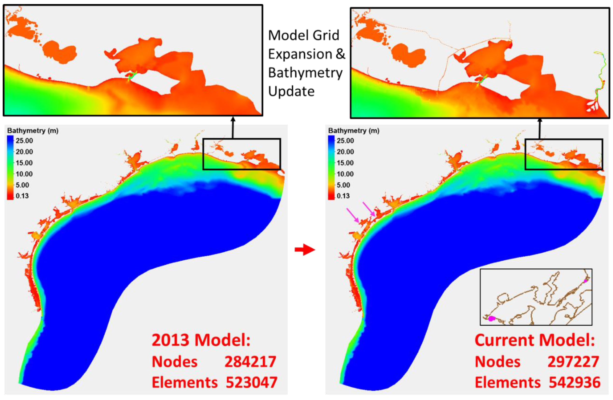
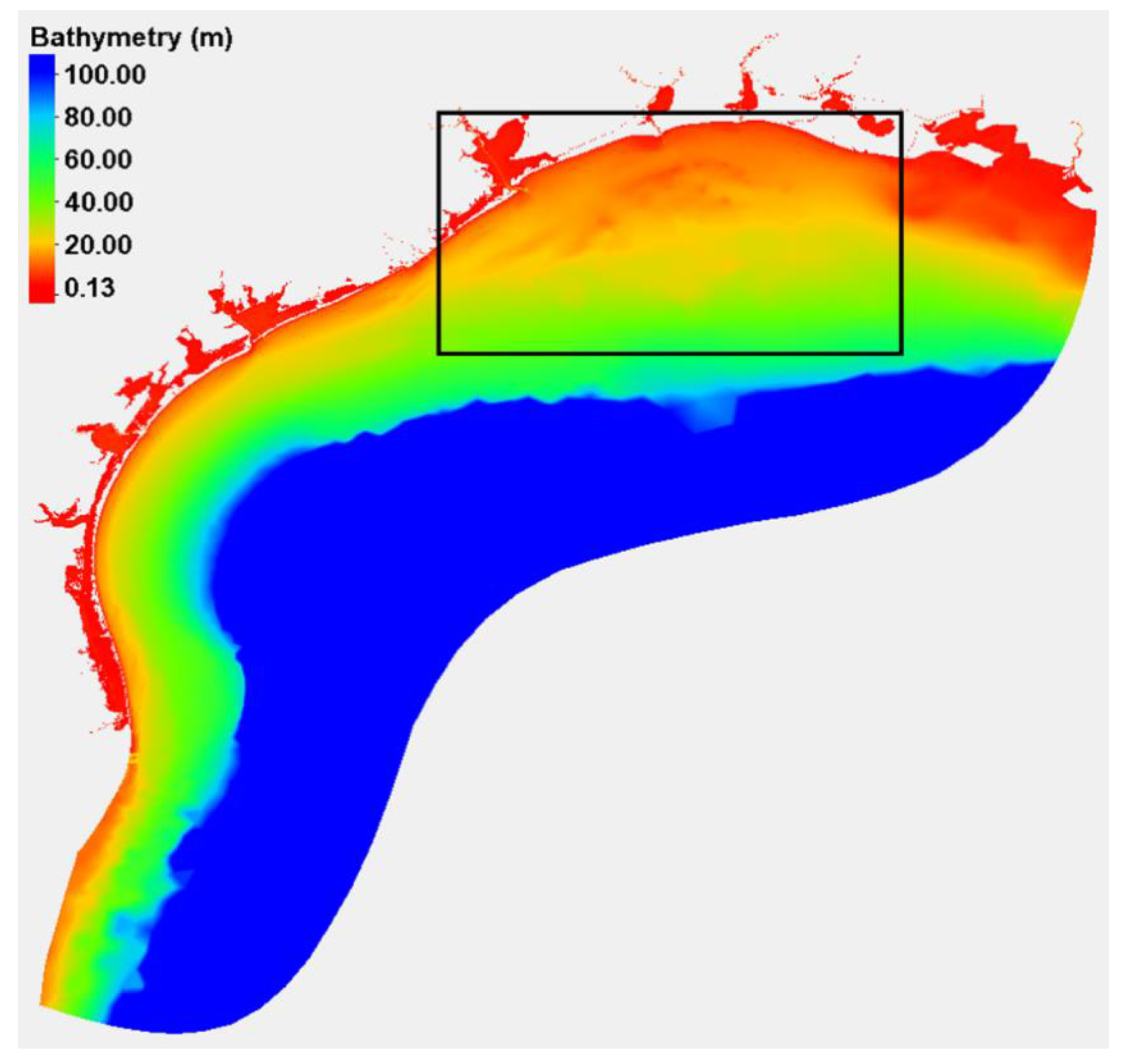
2.1.2. Model Domain

The model domain spans from the coast of San José de los Leones, Mexico [97.71° W, 24.25° N], about 198 km south of the US-Mexico border from Brownsville in the southwest of the model domain to the intersection of east of Caillou Bay and west of Lake Pelto [91.12° W, 29.22° N] in LA (Figure 1). The model domain was first extended to include new tide stations using a commercial software package called Surface-water Modeling System© [25] (SMS version 12.2.7). The major extension areas are in the western LA coastal region (Figure 2). Four new tide stations in the western LA coastal region were included through the extension. Two minor extension areas are in the middle of the TX coast to include two new tide stations (shown in the right panel of Figure 2): one is a shallow-water area in the southwest of Aransas River, and the other is a shallow and short water channel between Redfish Slough and Mustang Lake. It is worthwhile to note that the scope of the extension was determined by the judgment that water bodies in the extended areas were connected to the existing model grids and bathymetry was available.

NOAA’s shoreline dataset (Continually Updated Shoreline Product—CUSP [26]) was used as a reference for determining the model boundary when extending the model domain. Section 2.2.1 will give a brief introduction on the CUSP dataset and how we used the dataset.

The spatial resolution of the model grids ranges from 14.38 m in the coastal region to 28.58 km near the open ocean boundary. The updated model domain includes a total of 297,227 nodes and 542,936 elements. The grid resolution increases from the open ocean boundary to the coasts and embayments to better represent the complexity in the shorelines and shallow water tidal dynamics. The best available bathymetry data were used to update the model bathymetry. Model grid bathymetry ranges from 0.13 m to 2090.40 m. The shallowest bathymetry occurs in the lakes and the deepest bathymetry is located at the open ocean boundary. Section 2.2.2 will briefly describe the bathymetry datasets used for the update and their priorities.

2.2. Data

2.2.1. NOAA’s Continually Updated Shoreline Product (CUSP)

The shoreline represents a dynamic interface between land and water and it changes with time, as mentioned in Section 1. CUSP provides the most current shoreline representation of the U.S. and its territories, available online [26,27]. The CUSP shoreline dataset was created to deliver a continuous shoreline with frequent updates to support various applications, such as developing coastal and marine spatial plans; managing resources; mitigating hazard events; and conducting coastal environmental analyses for federal agencies, coastal state and local organizations, academic institutions, and private companies.

CUSP is built upon National Geodetic Survey’s (NGS’s) National Shoreline data and it uses all national shorelines that have been verified by contemporary imagery and shorelines from other non-NOAA sources including lidar, imagery, and shoreline vectors. The shoreline vector only includes shoreline and alongshore features that represent the shoreline (groins, breakwaters, and jetties). Individual national shoreline projects are edge matched using contemporary imagery as a guide. Single-line alongshore features and alongshore features where water passes underneath are not included. CUSP references a MHW shoreline based on vertical modeling or image interpretation using both water level stations and/or shoreline indicators if applicable. The decision to compile features is based on the ability to extract a proxy MHW line considering water level, image date, resolution, accuracy, and shoreline slope. CUSP covers the continental U.S., with portions of Hawaii, the Pacific Islands, Alaska, Puerto Rico, and the U.S. Virgin Islands.

We used the CUSP shoreline dataset as a reference to: (1) determine the model boundary when extending the model domain; and (2) update the coastline data file for producing the VDatum marine grid population.

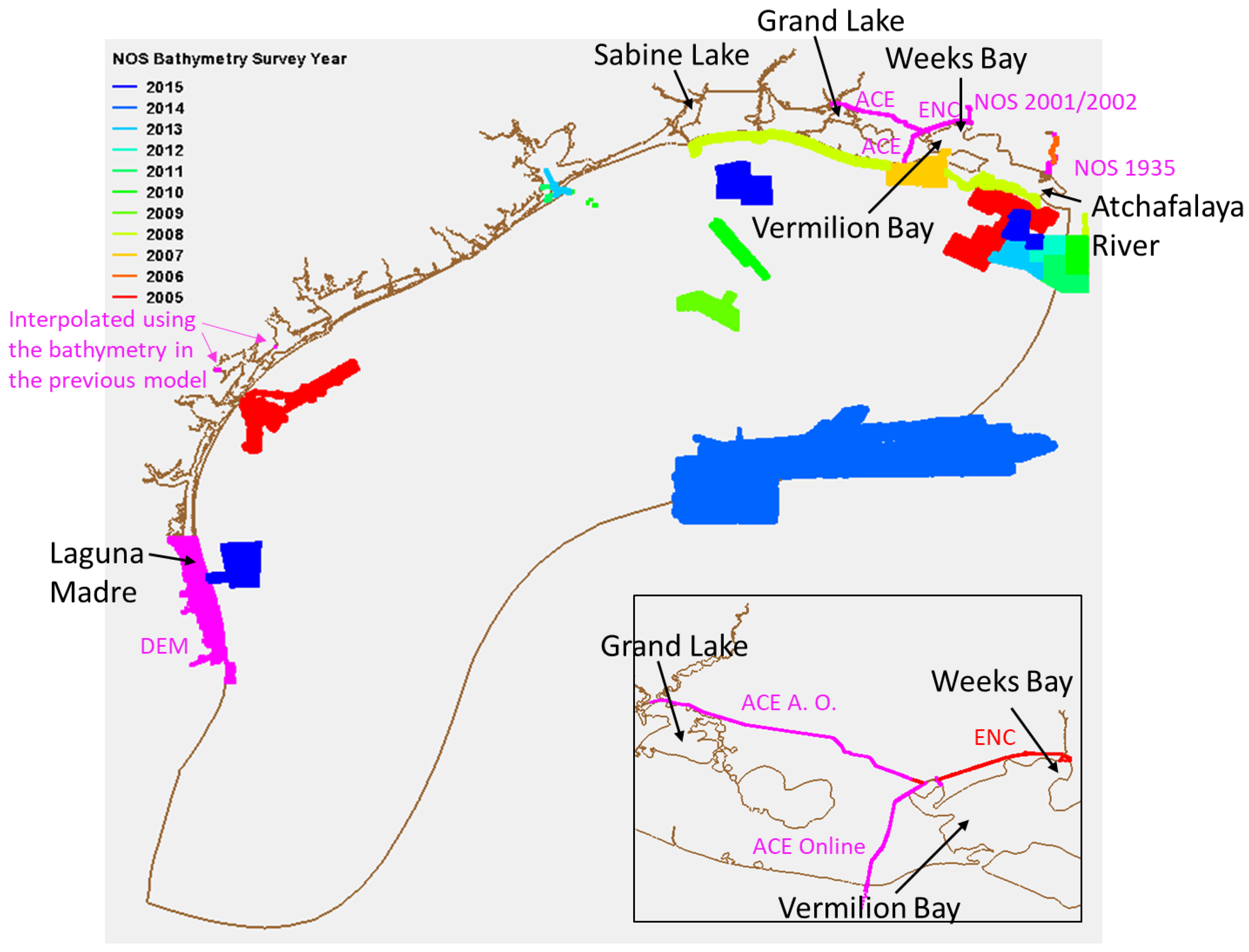
2.2.2. Bathymetry Data

Several bathymetry datasets were used to update the bathymetry for the model grids. Bathymetry data were applied by priority. The more reliable and more recent bathymetry data have a higher priority. For example, the most recent hydrographic survey data have the highest priority. The datasets used are listed below:

Priority 1. NOAA/NOS best available hydrographic survey data from 2005 to 2015, processed and provided by the data team at NOAA/NOS/OCS (Office of Coast Survey)/CSDL (Coast Survey Development Laboratory)/GADB (Geospatial Applications Development Branch). Note that NOAA/NOS older hydrographic survey data from 2001, 2002, and 1935 were also used for the extended waterways near Weeks Bay and Atchafalaya River (Figure 3), where no recent-year hydrographic survey data were available.

Priority 2. The U.S. Army Corps of Engineers (ACE) hydrographic survey data in the extended southern LA’s Freshwater Bayou area [28] and in the extended western LA’s ICW between Grand Lake and Vermilion Bay (Figure 3) (the 10-year accumulated bathymetry data in the area were kindly provided by ACE’s Andrew Oakman). No NOS hydrographic survey data were available in those areas.

Priority 3. NOAA’s Electronic Navigational Chart (ENC, Chart #11345) data [29] were used for interpolating bathymetry in the extended western LA ICW between Vermilion Bay and Weeks Bay where no hydrographic survey data were available.

Priority 4. NOAA’s National Geophysical Data Center (NGDC) High-Resolution Digital Elevation Model (DEM) data in the southwestern TX coastal area where no bathymetry data were available from the abovementioned three resources. The DEM bathymetry used for the model update is “South_Padre_TX_1/3_arc_second_DEM_MHW.asc” [30].

Priority 5. The previous model’s bathymetry dataset (the model input file “fort.14”) [7], which was created by using NOAA/NOS hydrographic survey data from 1885 to 2005, NOAA’s ENCs for Sabine Lake and southern Laguna Madre (Figure 3), and ACE bathymetry data (for major shipping channels and ICW in the previous model grids).

Figure 3 shows the locations, types, and years of the new bathymetry data used for the model update.

2.2.3. Observed Tidal Datums and Associated Root-Mean-Square (RMS) Errors

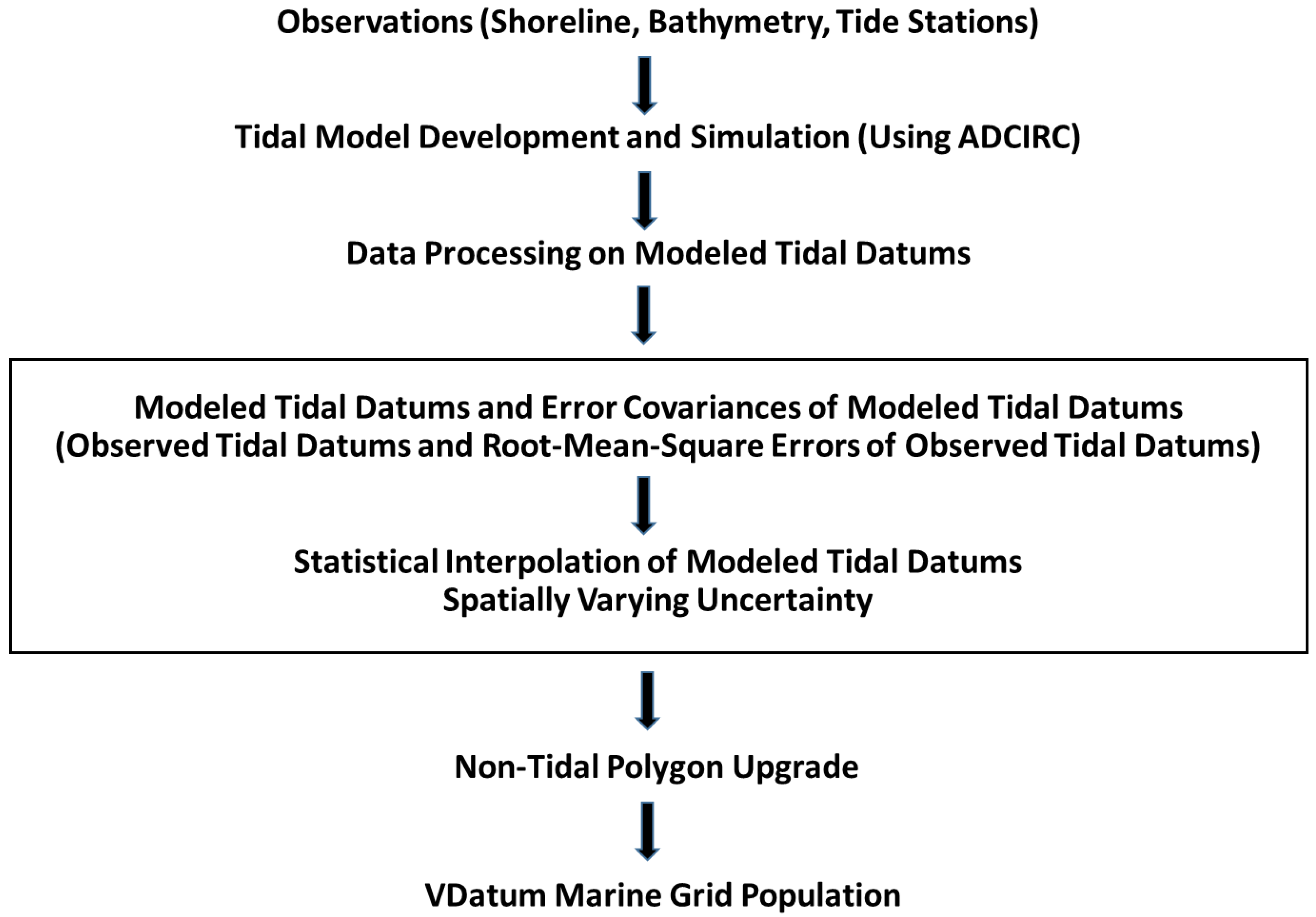
The observed tidal datums (MHHW, MHW, MLW, and MLLW) and associated RMS errors were calculated using observed water level time series at tide stations by CO-OPS [2,31]. The calculation method will be briefly introduced in Section 2.3.1. We used the observed tidal datums for assessing model performance, and used both the observed tidal datums and associated RMS errors for the statistical interpolation.

A total of 75 tide stations have valid greater-than-zero observed tidal datums within the model domain [98° W to 91° W, 24° N to 31° N]. Sixteen out of the 75 tide stations do not have the observed RMS error data, so we used the average of the RMS errors at the remaining 59 tide stations to represent the RMS errors in the 16 tide stations for the statistical interpolation. The locations of the tide stations will be shown later in Section 3.1 when we discuss the distributions of the observed tidal datums.

2.3. Methods

This section describes the methods used in the calculations of observed and modeled tidal datums, the SVU statistical interpolation, and the estimates of non-tidal zones. Figure 4 shows a schematic diagram which depicts the detailed workflow of the model update, with the statistical interpolation step enclosed within the box.

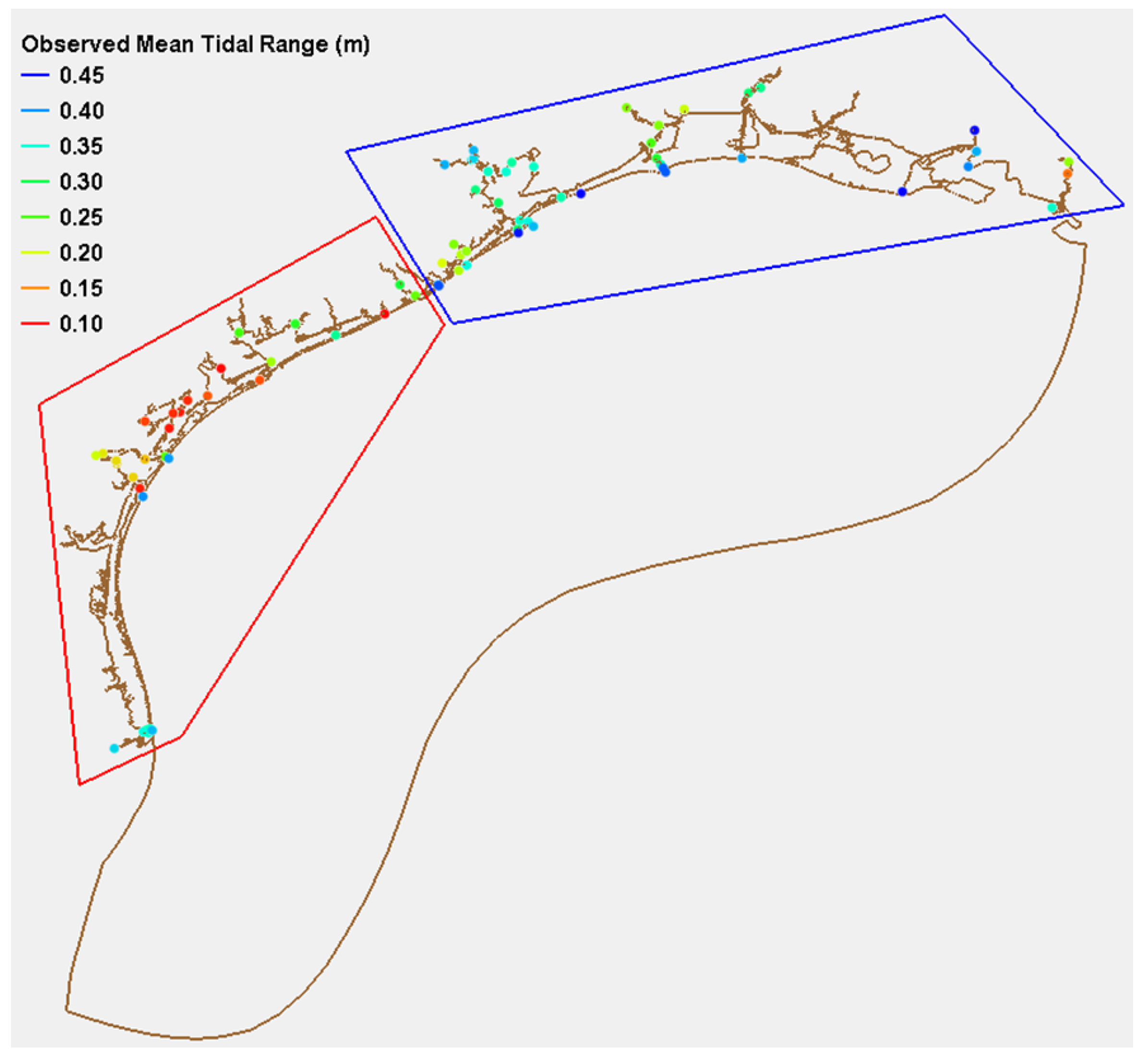
2.3.1. Calculation of Observed Tidal Datums

Detailed information about NOS observed datum computation procedures can be found in “CO-OPS’s Tidal datums and their Applications” [2,31]. NOS collects raw data at 6-min intervals from tide stations. The collected raw data were first processed for quality control. After that, the tabulation process with quality control was carried out, including the generation of hourly heights, high and low waters, and monthly means, and the selection of higher high and lower low waters. A specific 19-year period designated as a National Tidal Datum Epoch (NTDE) was used to compute tidal datums. The NTDE is used as the fixed period of time for the determination of tidal datums because it includes all significant tidal periods, it is long enough to average out the local meteorological effects on sea level, and specifying the NTDE can ensure a uniform approach to apply to the tidal datums for all stations. The current NOS observed tidal datums were computed with reference to the current tidal epoch of 1983–2001 NTDE.

Tidal datums at control stations are computed by an arithmetic mean method for a specific length of record over a tidal epoch. The input for the procedure requires the monthly mean values for a tidal epoch. Tidal datums at secondary stations are generally computed by a comparison of monthly means between subordinate and control stations. Tidal datums at tertiary stations are computed by a comparison of monthly means or comparison of simultaneous high and low waters (if no calendar month of data) between the tertiary station and a control station, or with an acceptable secondary station. The input for this procedure is the simultaneous means from the control and subordinate stations in a region of similar tidal characteristics to produce an equivalent datum at the subordinate station with an adjustment to 19-year values. More details about observed datum computation can also be found in [2,31,32,33,34].

2.3.2. Calculation of ADCIRC Tidal Datums

Detailed procedures about how modeled datums were computed by using the 6-min ADCIRC modeled water level time series can be found in “Standard Procedures to Develop and Support NOAA’s Vertical Datum Transformation Tool” [5].

First, modeled water level time series are checked for several conditions, including too small a signal, drying or ponding, and repeated values. For example, if a model node goes dry (i.e., its water depth drops below some specified value h0), the model code automatically substitutes a default value for the output elevation. Thus, the first check is for water level values below a user-defined level h99. If this situation has occurred, the analysis is skipped and the output values of the datums are set to be a default value.

After that, the averaged water levels for each half-hourly period (centered on the hour and half-hour) are computed to estimate the times of tidal peaks by following a specific approach and by using the method of singular value decomposition [5]. Peaks are then put into chronological order and any repeated peaks are eliminated.

Next, the peaks are screened and those pairs that do not fit separation criteria are eliminated. CO-OPS’ criteria are that the amplitudes must differ by at least delhr in time (hours) and delamp in amplitude (meters), where the nominal values delhr = 2.0 h and delamp = 0.03 m were used in this work. First, extrema pairs are screened and those too close in time are eliminated. Then, in the standard procedures, the mean tidal range, which is computed as the difference between the mean of the high waters minus the mean of the low waters, is checked. If this range is lower than a user-specified value rangemin, datums for that time series are set to be a default value. Then, extrema pairs are screened and those too close in amplitude are eliminated. Then, another check of the mean tidal range is made.

Following this, the highs and lows are separated into higher highs, lower highs, higher lows, and lower lows by applying the ‘25 h algorithm’ developed by CO-OPS. For example, three successive highs in a 25-h window are examined to determine the maximum value. The window is then centered on this peak, which becomes the higher high; the peaks ahead and behind become lower highs. Finally, in the last step, all the higher highs are averaged to determine the Mean Higher High Water (MHHW), all the daily lower highs are averaged to determine the Mean Lower High Water (MLHW), and all the peaks are averaged to become the Mean High Water (MHW). The calculations for low water are analogous. The Mean Tide Level (MTL) is the mean of MHW and MLW, and the Diurnal Tide Level (DTL) is the mean of MHHW and MLLW. Note that modeled Mean Sea Level (MSL) is the mean of the 6-min modeled water levels. The MSL was deducted from the six tidal datums for a comparison with the observed tidal datums which have also deducted the observed MSL.

2.3.3. Statistical Interpolation of Tidal Datums and Their Associated Spatially Varying Uncertainties

Once the ADCIRC modeled tidal datums are derived from the 6-min modeled water level time series, a tidal datum analysis field f is calculated by blending the modeled tidal datum with observed tidal datum using a statistical interpolation method [13].

As described in “Statistical Interpolation of Tidal Datums and Computation of Its Associated Spatially Varying Uncertainty” [13], the method was developed based on the variational principle. We first constructed a cost function $J\left(f\right)$ according to the statistical characteristics (error covariance) of the observed and modeled tidal datums as

$$J\left(f\right)=\frac{1}{2}{\left(f-f_m\right)}^T{P}^{-1}\left(f-f_m\right)+\frac{1}{2}{\left(f_0-Hf\right)}^T{\left(W^{-\frac{1}{2}}\right)}^T{R}^{-1}{W}^{-\frac{1}{2}}\left(f_0-Hf\right)$$

(1)

where $f$ is a new $n$ × 1 tidal datum analysis field at model mesh nodes, $f_m$ is a size $n$ × 1 discrete modeled tidal datum field, $f_0$ is a size $m$ × 1 observed tidal datum field at CO-OPS station locations, H (size $m$ × $n$) is the interpolation matrix projecting the modeled field to the observed data locations, and W (size $m$ × $m$) is a diagonal weight matrix that adjusts how much the final product $f$ differs from the observed values at the station locations. It is assumed the model and observation fields are unbiased, and both $f_m$ and $f_0$ follow a normal distribution, where Var($f_m$) = $P$ and Var($f_0$) =$R$, respectively. Then, we derived a blended tidal datum field $f$ that minimizes the cost function $J\left(f\right)$ as

$$f=f_m+G\left(f_0-H{f}_m\right)$$

(2)

where $G=P{H}^T{[W^{\frac{1}{2}}R{\left(W^{\frac{1}{2}}\right)}^T+HP{H}^T]}^{-1}$ is the gain matrix and $f$ is the unbiased estimate of the true tidal datum field. In the final step, as a by-product, the associated uncertainty (e.g., the posterior error covariance matrix $P_a$) is calculated for the blended tidal datum field $f$ by

$$P_a=Var\left(f\right)=\left(I-GH\right)P{\left(I-GH\right)}^T+GR{G}^T$$

(3)

where $I$ is the identity matrix.

Note that the model error covariance matrix is estimated as $P_{ij}=var\left(f_{n_1},f_{n_2}\right)={\sigma }_{n_1}{\sigma }_{n_2}corr\left(f_{n_1},f_{n_2}\right),$ (1 ≤ $i,j$ ≤ $n$, in unit of m²). ${\sigma }_{n_1}$ and ${\sigma }_{n_2}$ are the standard deviations of the model errors at nodes $n_1$ and $n_2$, respectively, and are assumed to be constant at all the model nodes which were equal to the standard deviation of the modeled errors at all the tide stations. The correlation between two points is calculated using a three-day moving average tidal datum time series. Here, the covariance is adjusted and decreases exponentially over the distance between nodes $n_1$ and $n_2$. Also, the weight matrix $W$ determines the weight of $R$ in the computation of the analysis field $f$. The diagonal element $w_{ii}$ (0 ≤ $w_{ii}$≤ 1, 1 ≤$i$ ≤$m$) is the weight of the observation error variance $r_{ii}$ at station $i$ in the determination of analysis field $f$. The weight matrix $W$ was determined through iteration following the predetermined constraint; that is, the discrepancy between the analysis field and the observations at all tide stations is equal to or less than 1 cm or the CO-OPS’s uncertainty value (observed rms error), whichever is less.

As demonstrated in [13], the statistical interpolation has a few advantages over the traditional deterministic correction method: (1) it provides a spatially varying uncertainty; (2) it provides a framework to assimilate future data streams with known uncertainty to improve the quality of the final tidal datum product; and (3) it reduces model bias, maximum absolute model error, mean absolute model error, and root mean square of the model errors in comparison with the traditional deterministic approach.

The traditional method for correcting modeled tidal datums, called “Tidal Constituent and Residual Interpolation (TCARI)”, was based on the application of Laplace’s Equation [5,35,36,37]. The TCARI method numerically creates a tidal datum correction field at all the model grid points by using the modeled tidal datum errors at tide stations. The modeled tidal datums after TCARI corrections closely match the observed tidal datums at tide stations. The accuracy (uncertainty) of the modeled tidal datums after TCARI corrections was assessed by computing the root mean square of the differences between the observed value and the TCARI-interpolated value over an entire interested model domain, which was obtained by using a jackknifing approach and the TCARI method. A detailed explanation of the estimation of the VDatum uncertainty can be found in [5,38].

It is worth pointing out that the RMS error of the observed tidal datum at each tide station is the same for all the tidal datums. The difference in tidal datums’ spatially varying uncertainties mainly comes from the difference in the covariance of the modeled tidal datum errors, which is different for different tidal datums.

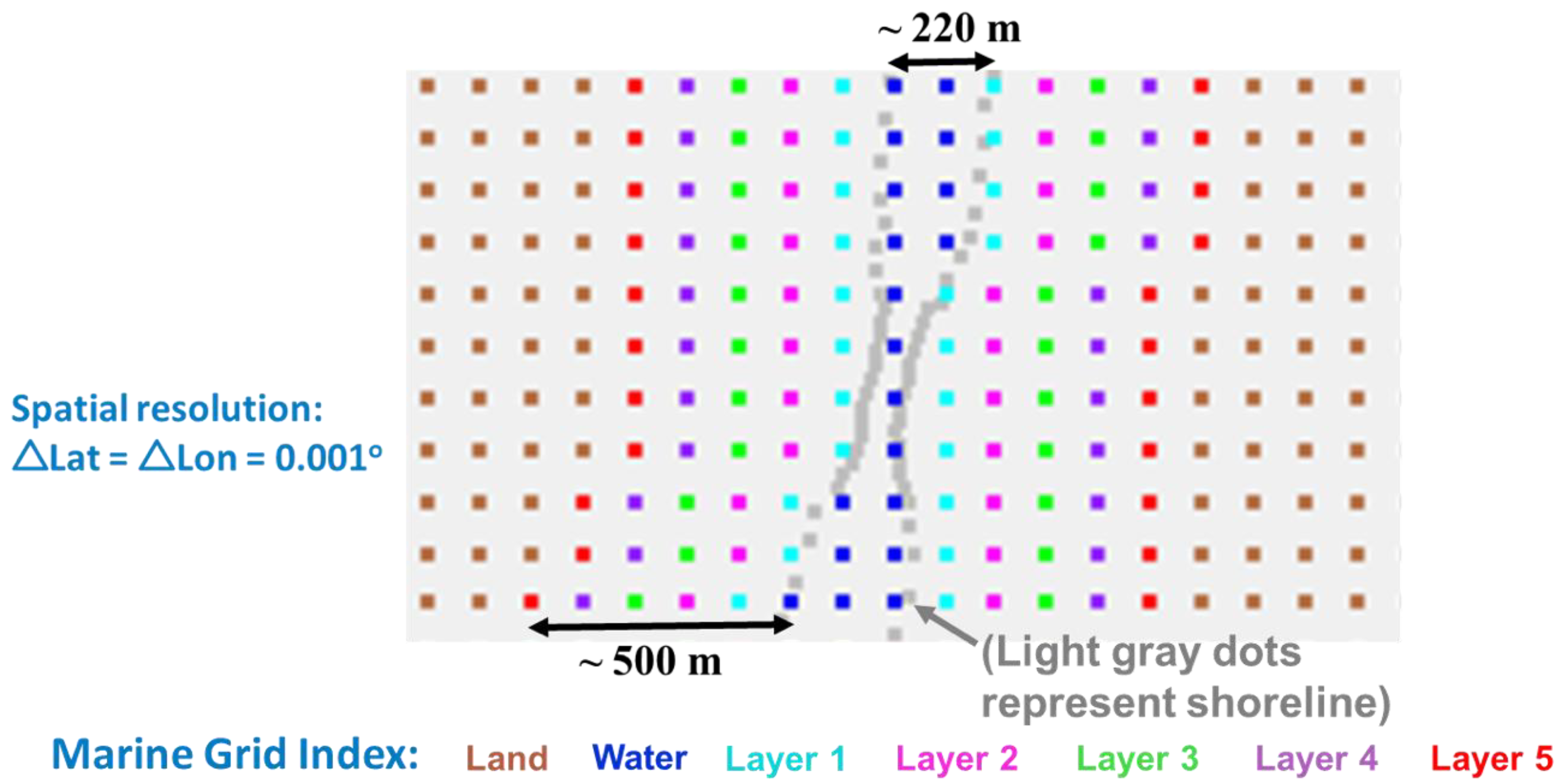
2.3.4. Estimates of Non-Tidal Zones and VDatum Marine Grid Population

As mentioned in Section 1, CO-OPS established the “non-tidal” zones, which represent areas where a periodic tide is present and consistent in the observations, but the mean tidal range is negligible (MHW minus MLW is less than 0.09 m) [14]. Likewise, a model grid point referred to a modeled non-tidal grid if its modeled MHW minus MLW was less than 0.09 m. Modeled non-tidal grids were incorporated for upgrading the existing non-tidal polygons (detailed in Section 3.4).

The upgraded non-tidal polygons were used for the VDatum marine grid population (the last step of the workflow, as shown in Figure 4) to ensure the areas with valid tidal datums have valid populated tidal datums at marine grids, while the areas without valid tidal datums (non-tidal areas) have invalid populated tidal datums at marine grids. The VDatum marine grid population includes two steps [5]: First, a uniformly spaced marine grid field was generated with a spatial resolution of 0.001 (one thousandth) degree in longitude and latitude (see an example in Section 3.4). The marine grid field distinguishes between points that represent land and those that represent water, using a coastline and bounding polygon file to make the determination. Then, the marine grids were populated using modeled tidal datums.

The accuracy of non-tidal polygons is thus crucial to the quality of the VDatum marine grid population. The important role of non-tidal polygons in the VDatum marine grid population will be explained in Section 3.4. In this work, we incorporated the modeled non-tidal grids to upgrade the existing non-tidal polygons for enhancing the quality of the VDatum marine grid population.

3. Results and Discussion

3.1. Observed Tidal Datums

Figure 5 shows the four major tidal datums from observations at the 75 available tide stations in this model domain. The observed tidal datums are referenced to the local MSL at each station. As introduced in Section 1, MHHW/MHW/MLW/MLLW respectively refer to the average of the higher high water height each tidal day, the average of all the high water heights each tidal day, the average of all the low water heights each tidal day, and the average of the lower low water height each tidal day.

As shown in this figure, the maximum value of the observed tidal datums in the model domain is less than 0.40 m. The observed tidal datums show relatively larger values from the Houston area to the east: MHHW and MHW are greater than 0.10 m, and MLW and MLLW are deeper than −0.20 m. The area from Houston to the west shows relatively smaller tidal datums.

Figure 6 shows the mean tidal ranges from the 75 tide stations, ranging from 0.10 m to 0.49 m. The mean tidal range from Houston to the east is much larger than that from Houston to the west. The averaged value of the observed mean tidal ranges equals 0.33 m for the region from Houston to the east (blue polygon) and 0.23 m for the region from Houston to the west (red polygon). It is worthwhile to mention that the Gulf of Mexico is characterized as a region with a small tidal range. This is mainly because: (1) the Gulf of Mexico has a narrow connection with the Atlantic Ocean; and (2) the Gulf of Mexico is a diurnal-tide dominant ocean basin, but the diurnal tides are small in the Atlantic Ocean since the Atlantic Ocean is too small to produce resonant sloshing with a diurnal-tide period [39].

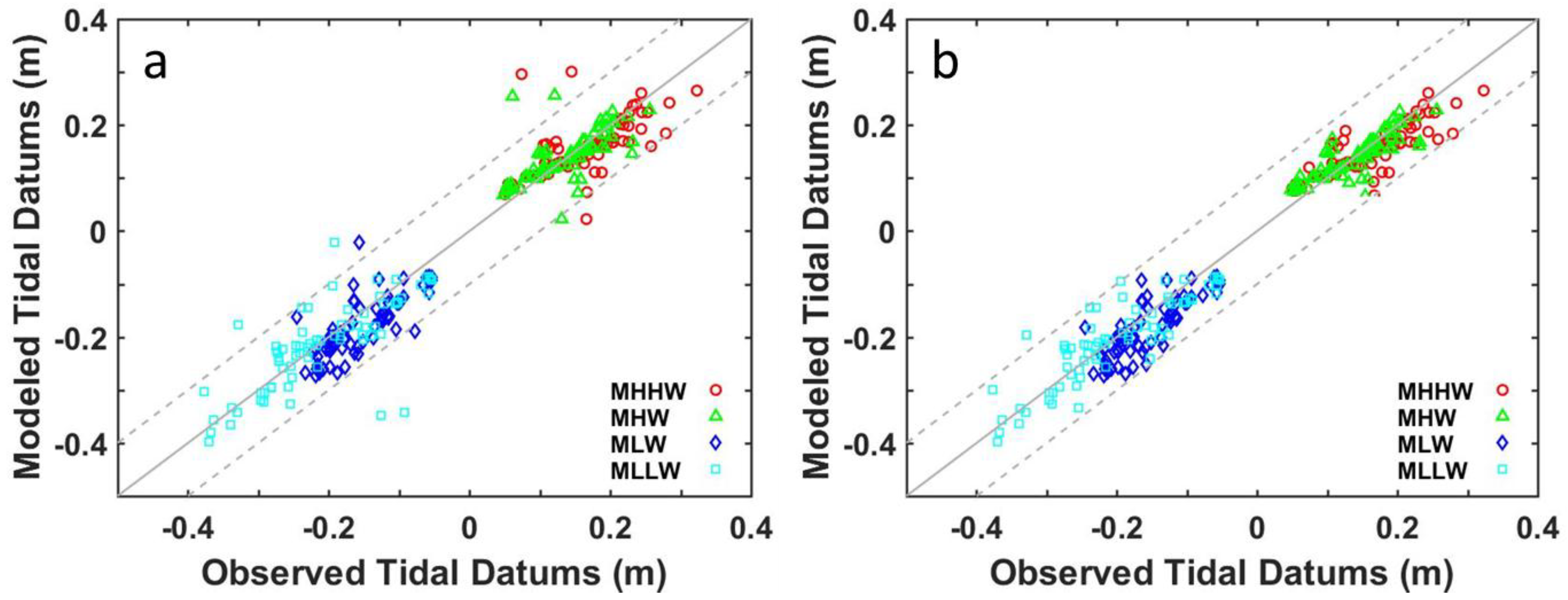
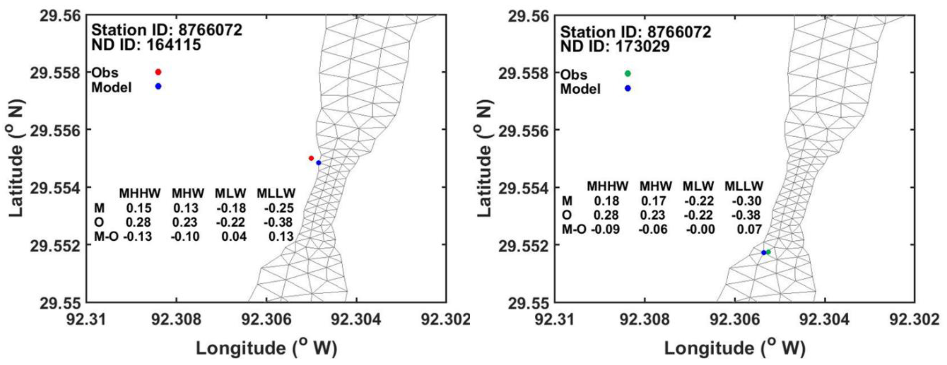
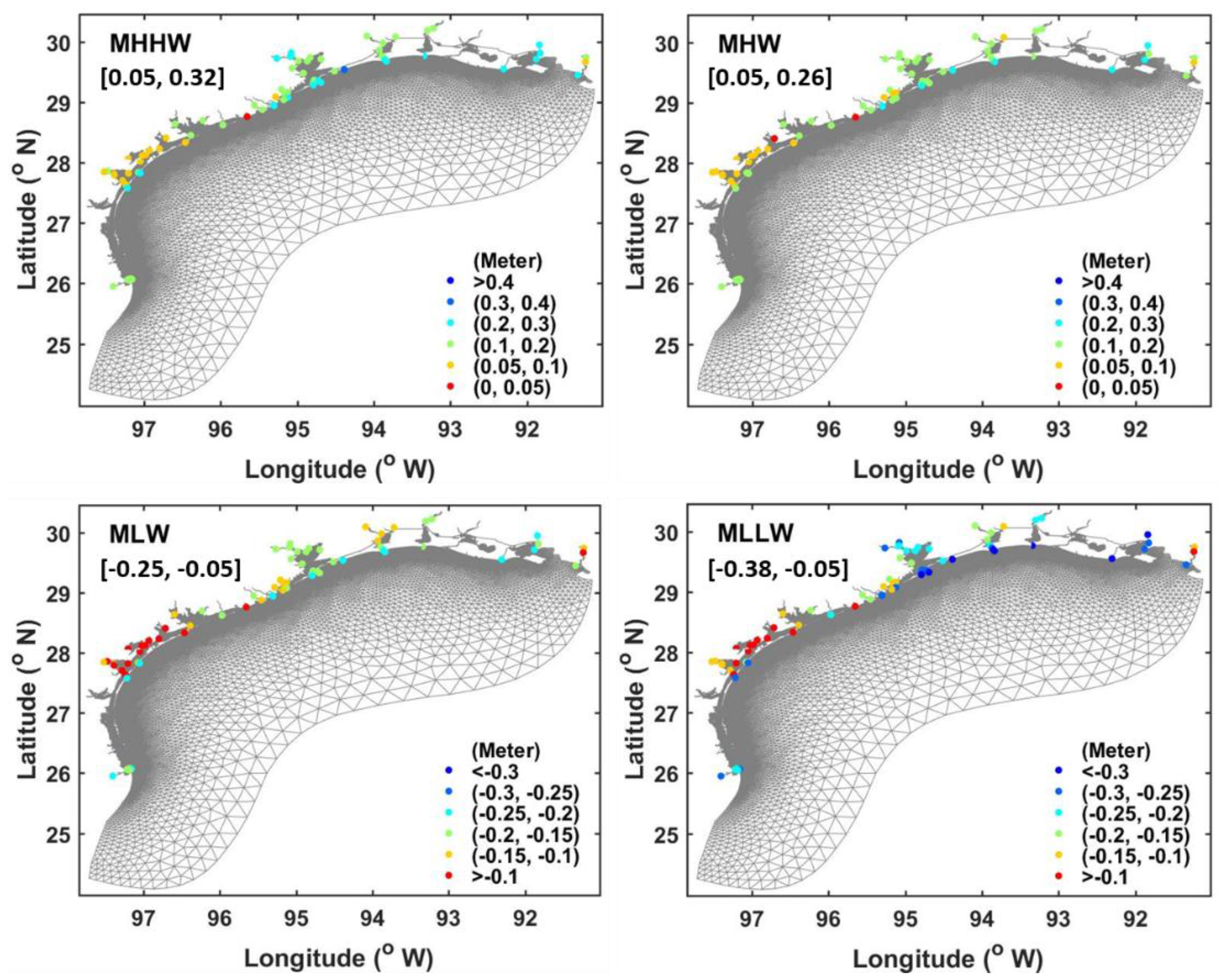
3.2. The Assessment and Improvement of ADCIRC Modeled Tidal Datums

Figure 7a shows a comparison between the ADCIRC modeled tidal datums and the observed tidal datums. The modeled tidal datums at four tide stations have greater than 0.10 m model errors. The 0.10 m threshold set was determined by considering this region’s small tidal range, the experience of the previous model, and the magnitude of the observed RMS errors in this region.

According to the geographic characteristics of the four tide stations, sensitivity tests were conducted and the model performance was significantly improved after model adjustments (Figure 7b). The effective techniques used for model improvement include: (1) extending the river length in the upper streams (for fixing model overestimation); (2) refining the model grid near a river’s entrance, for example, enhancing model grid resolution and removing land patches from a model element (for fixing model overestimation); (3) increasing the model grid resolution along rivers (for fixing model underestimation); (4) enhancing the width of a narrow river (for fixing model underestimation); and (5) correcting bathymetry near a river’s entrance (for fixing model underestimation).

An important lesson learned from the model assessment is that the accuracy of a station’s coordinates is critical. As an example, Figure 8 shows the model errors of the four major tidal datums at one specific tide station before (left) and after (right) the station coordinates were corrected.

In the left panel, the model errors are greater than 0.10 m for MHHW and MLLW, and the station’s coordinates [92°18.3′ W, 29°33.3′ N] correspond to a land location (inaccurate). After correction, the true station’s coordinates (the right panel) are [92°18.315720′ W, 29°33.105300′ N]. Although the errors from the coordinates are small: delta (longitude) = −0.01572′ W and delta (latitude) = 0.1947′ N, which yield a distance of about 350 m in between, the true model errors of the tidal datums reveal much smaller values (<0.10 m), as shown in the right panel. The accuracy of the station’s coordinates is essential to making an effective model assessment and thus to producing accurate modeled tidal datums. Discussions on the significance of the Earth surface coordinates’ accuracy to ensure good-quality nautical, navigational, and geospatial products are also given in [40].

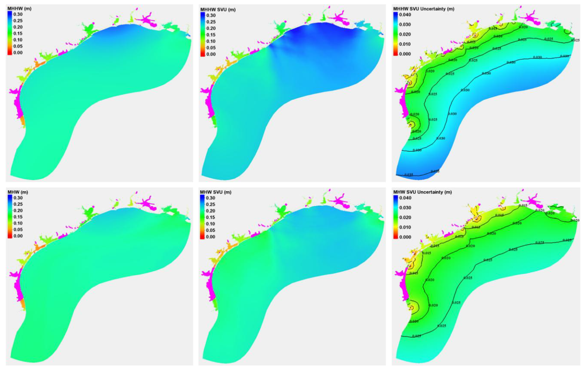
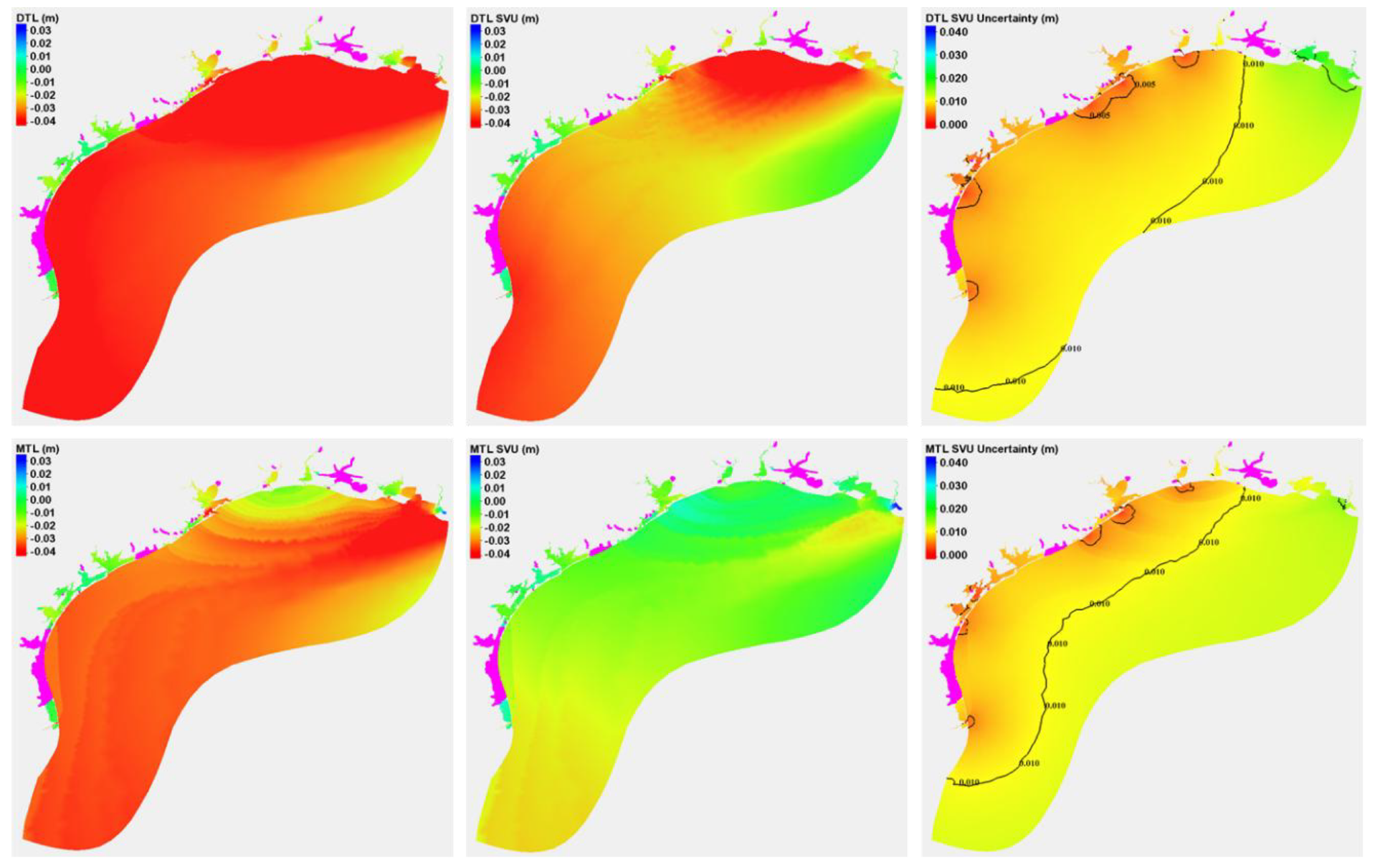
3.3. Statistical Interpolation of Modeled Tidal Datums and Associated Uncertainties

ADCIRC modeled tidal datums, and the modeled tidal datums after the SVU statistical interpolation and their associated SVU spatially varying uncertainties of MHHW/MHW, MLW/MLLW, and DTL/MTL are shown in Figure 9, Figure 10 and Figure 11, respectively. Modeled non-tidal grid points in the figures are marked as pink dots. As we will show later, the modeled non-tidal grid points in general agree with the CO-OPS estimated non-tidal zones.

Similar to the observed tidal datums, the modeled tidal datums (except for MLW and DTL with relatively uniform distributions) show relatively larger values in the eastern coastal region than in the western coastal region. The distributions of the modeled MHHW, MLLW, and MTL are qualitatively consistent with the characteristics of the observed proportion of tidal current energy to total energy (Figure 3 of [41]) and of the observed mean amplitude of tidal current energy (Figure 16 of [41]) from the same eight principal tidal constituents (K1, O1, P1, Q1, M2, S2, N2, and K2); that is, a rapid increase in magnitude from about 130 km offshore to the northern Texas-Louisiana shelf and from the Houston area to the east, within [95.5° W to 92.3° W, 28.5° N to 29.8° N]. It is worthwhile to mention that the analyzed tidal current observations were limited to only offshore stations; that is, no tidal current observations are close to the shore. Both the abovementioned distributions of the modeled tidal datums and the characteristics of the tidal current observations show roughly uniform patterns across the southern Texas shelf west of Houston, with a minor decrease in magnitude farther offshore. Similar patterns were also found in the previous modeled tidal datums, as shown in Figure 10 of [7]. The concave geographic shape of the basin and the large water body with shallow bathymetry (Figure 12) in the northern Texas-Louisiana shelf (within the black box) could be one of the major triggers of the relatively larger tidal datums and tidal current energy, in addition to the dominant loop currents in the Gulf of Mexico, as shown in Figure 1 of [42].

Figure 9 and Figure 10 show that the spatially varying uncertainty of the four major tidal datums computed by the SVU statistical interpolation method is the largest for MLLW, the second largest for MHHW, the third largest for MLW, and the smallest for MHW. The spatially varying uncertainty was smaller at nodes close to the coastal lines and tide stations, and was relatively larger otherwise. The largest uncertainties were located near the open ocean boundary, where no tide stations existed and the distance to the available tide stations was the greatest. As stated in Section 2.3.3, the RMS errors of the observed tidal datums at each tide station were the same for all the tidal datums. The difference among tidal datums’ spatially varying uncertainties was mainly determined by the difference in the model error covariance ${\sigma }_{n_1}{\sigma }_{n_2}corr\left(f_{n_1}, f_{n_2}\right)$, which was different for different tidal datums. Note that ${\sigma }_{n_1}$ and ${\sigma }_{n_2}$ were the standard deviations of the model errors at nodes $n_1$ and $n_2$, respectively, and were assumed to be constant at each node and equal to the standard deviation of the modeled errors at all the tide stations. Here, the covariance was adjusted and decreases exponentially over the distance between nodes $n_1$ and $n_2$, as mentioned in Section 2.3.3. Thus, the MLLW has the greatest uncertainty, mainly because it has the largest model background error (the standard deviation ${\sigma }_n$ of the model errors at all the tide stations). The standard deviation ${\sigma }_n$ of the model errors at tide stations (from the largest to the smallest) is 0.0417 m (MLLW), 0.0347 m (MHHW), 0.0327 m (MLW), or 0.0281 m (MHW). Also, because the covariance was adjusted and decreases exponentially over the distance between nodes $n_1$ and $n_2$, the greater the distance from a node to tide stations, the larger the SVU uncertainty at the node, which explains why the greatest uncertainty was located near the open ocean boundary.

The statistical values of the observed, ADCIRC modeled, and SVU statistical interpolated MHHW/MHW/MLW/MLLW tidal datums and associated SVU uncertainties are listed in

Table 1. Statistical values of observed and modeled tidal datums and the associated SVU spatially varying uncertainties (in meters). Model errors from observations are given in parentheses when applicable; note that errors do not necessarily correspond to the categorical value reported next to them (e.g., min, max, mean), but are instead the categorical error over the entire model domain. For example, the maximum model error (0.063) next to the maximum value of ADCIRC modeled MHHW (0.28) refers to the maximum model error of ADCIRC modeled MHHW in comparison with the observations at the 75 tide stations. Note also: Model errors refer to modeled tidal datums minus observed tidal datums; “Mean Value” of ADCIRC model errors refers to Mean (Abs(ADCIRC model error)); “Mean Value” of ADCIRC-SVU model errors refers to Mean (Abs(ADCIRC-SVU model error)); “STD” stands for Standard Deviation.

Data Type	MHHW	MHW	MLW	MLLW
		Maximum Value
Observation	0.32	0.26	−0.25	−0.38
ADCIRC	0.28 (0.063)	0.24 (0.067)	−0.31 (0.072)	−0.43 (0.132)
ADCIRC-SVU	0.31 (0.010)	0.25 (0.010)	−0.27 (0.010)	−0.45 (0.010)
SVU Uncertainty	0.036	0.033	0.034	0.046
		Minimum Value
Observation	0.05	0.05	−0.05	−0.05
ADCIRC	0.03 (−0.010)	0.03 (−0.088)	−0.03 (−0.093)	−0.03 (−0.089)
ADCIRC-SVU	0.03 (−0.010)	0.03 (−0.010)	0.00 (−0.010)	−0.03 (−0.010)
SVU Uncertainty	0	0	0	0
		Mean Value
Observation	0.16	0.14	−0.15	−0.20
ADCIRC	0.16 (0.028)	0.15 (0.021)	−0.18 (0.035)	−0.21 (0.032)
ADCIRC-SVU	0.17 (0.005)	0.15 (0.005)	−0.16 (0.005)	−0.22 (0.005)
SVU Uncertainty	0.015	0.013	0.015	0.018
		STD
Observation	0.066	0.052	0.053	0.090
ADCIRC	0.066 (0.035)	0.056 (0.028)	0.074 (0.033)	0.102 (0.042)
ADCIRC-SVU	0.069 (0.006)	0.055 (0.006)	0.057 (0.007)	0.095 (0.006)
SVU Uncertainty	0.004	0.004	0.005	0.006

. “Max”, “Min”, “Mean”, and “Std” represent the maximum, minimum, mean, and standard deviation, respectively. “Abs” refers to an absolute value. “ADCIRC-SVU” refers to the modeled tidal datums after SVU statistical interpolation, and “SVU uncertainty” refers to the spatially varying uncertainty values. Tidal datums are in a 2-decimal form, errors/standard deviations are in a 3-decimal form, and all are in the units of meters.

Table 1 reveals the small tidal datums in this model domain. The observed tidal datums (located only in coastal regions) are less than 0.38 m, the ADCIRC modeled tidal datums (in the entire model domain) are less than 0.43 m, and the tidal datums after the SVU interpolation are less than 0.45 m. The spatially varying uncertainties of the tidal datums after the SVU statistical interpolation are less than 0.046 m. It is worth mentioning that the MLW and MLLW datums are negative and thus the minimum values of the MLW and MLLW datums refer to the shallowest MLW and MLLW datums.

The magnitude of the ADCIRC model error is the greatest for the MLLW datum and the smallest for the MHHW datum. The mean absolute ADCIRC model error is the greatest for the MLW datum and the smallest for the MHW datum.

The modeled tidal datums after the SVU statistical interpolation are close to the observed tidal datums at all the tide stations to less than 0.010 m. The mean value of the SVU uncertainty is the greatest for the MLLW datum and the smallest for the MHW datum. Likewise, the maximum value of the SVU uncertainty is the greatest for the MLLW datum and the smallest for the MHW datum.

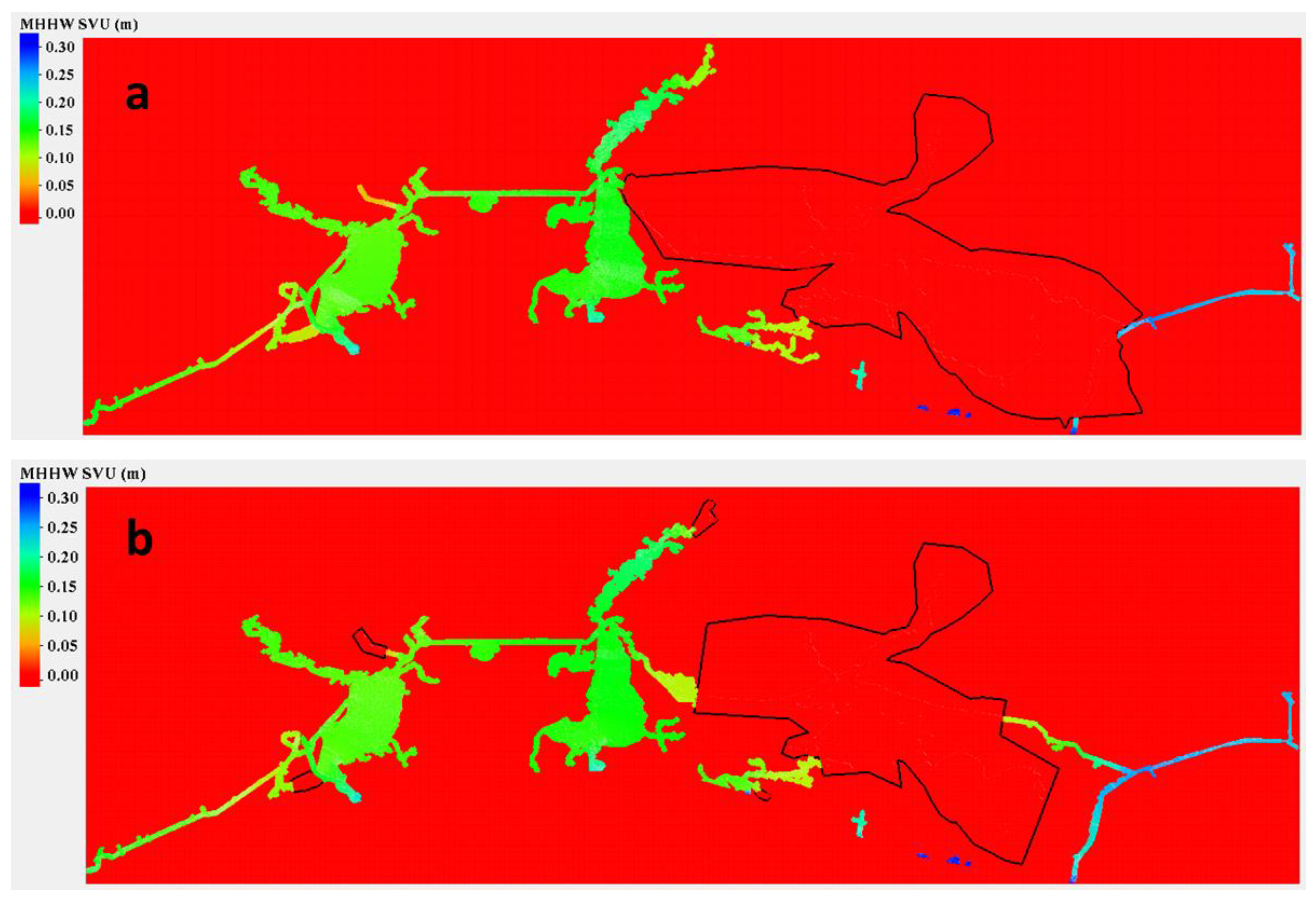
3.4. Non-Tidal Polygon Upgrade and VDatum Marine Grid Population

Modeled non-tidal grids were incorporated for upgrading existing observationally-based estimates of non-tidal polygons produced by CO-OPS (shown in the left panel of Figure 13). The non-tidal polygons after the upgrade are shown in the right panel of Figure 13. As shown in the figure (the left panel), the ADCIRC modeled non-tidal zones (pink dots) in general agree with the CO-OPS estimated non-tidal polygons (closed black lines).

For upgrading the CO-OPS estimated non-tidal polygons, modeled non-tidal grids were incorporated in the areas without or lacking tidal observations, such as the western LA coastal region (Area 1) and the middle TX coastal region (Area 2). We kept the CO-OPS estimated non-tidal polygons unchanged for areas where CO-OPS has tidal observations or references, but the model missed predicting non-tidal information, such as part of the Houston coastal region (the non-tidal polygons between Area 1 and Area 2) and part of the southwestern TX coastal region.

The major adjustments include: (1) a significant reduction in non-tidal area and four new small non-tidal areas in the western LA coastal region (Area 1); and (2) a significant extension in non-tidal area and several new non-tidal areas in the middle TX coastal region (Area 2).

The accuracy of non-tidal polygons directly influences the quality of the final VDatum marine grid population. Figure 14 shows an example of the VDatum marine grid population for the modeled MHHW after the SVU interpolation in the western LA coastal region by using the non-tidal polygons before (Figure 14a) and after (Figure 14b) the upgrade. As can be seen, the populated MHHW does not have any values inside the polygons. Using the existing non-tidal polygons causes several areas with valid tidal datums to be excluded in the final valid VDatum product. This is because the existing non-tidal polygons cover part of the region with valid tidal datums that prohibits the generation of a complete picture of the VDatum marine grid population. On the contrary, the upgraded polygons enable the VDatum marine grid population to reveal a complete picture of the datum. Thus, the upgrade of the non-tidal polygons enhanced the quality of the VDatum marine grid population.

It is worthwhile to mention that five water layers were artificially added landward from the shoreline in the marine grid generation, equivalent to a total distance of about 500 m or greater in this model domain, as shown in Figure 15. The five artificially added water layers allow datums to extend artificially to land for people who need the datum information.

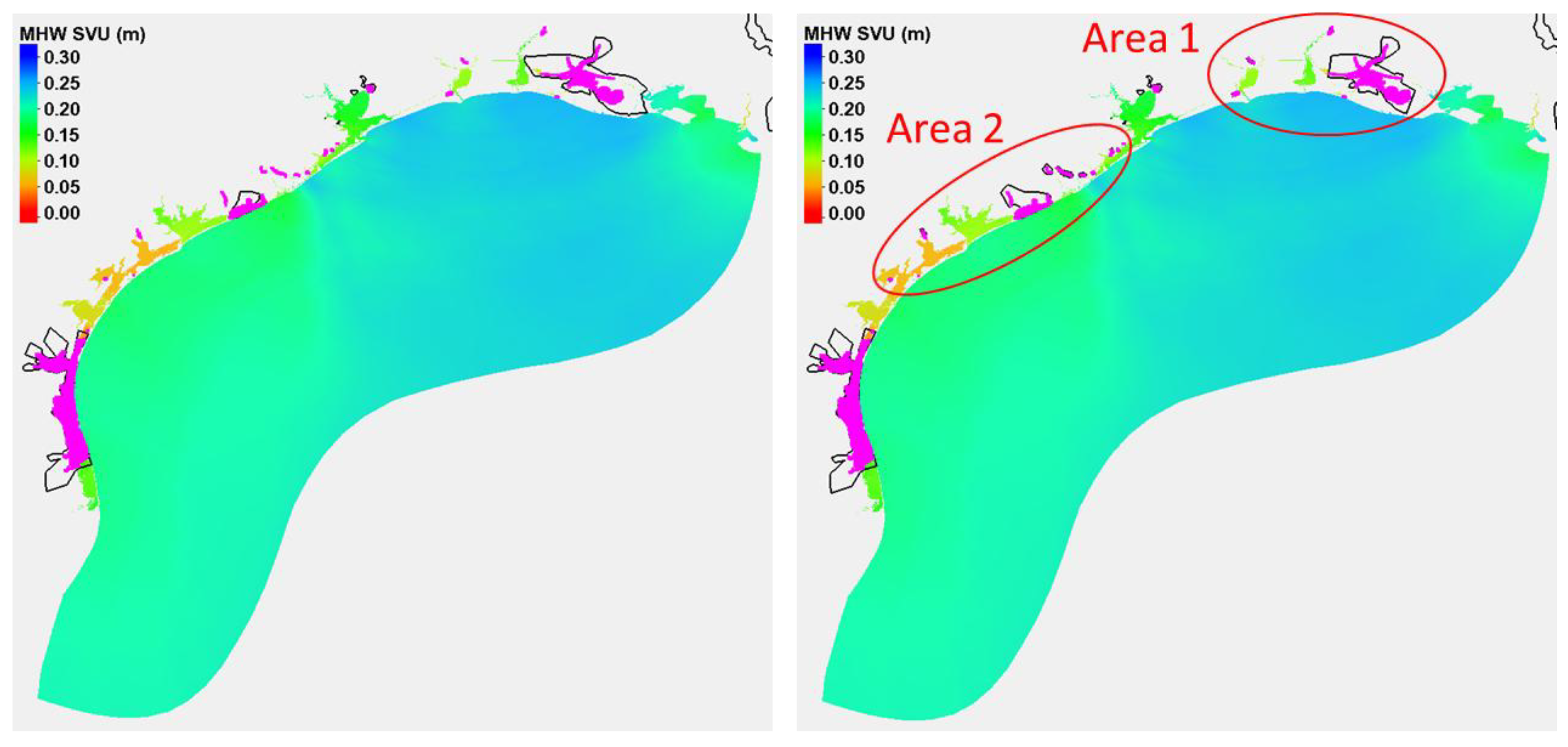
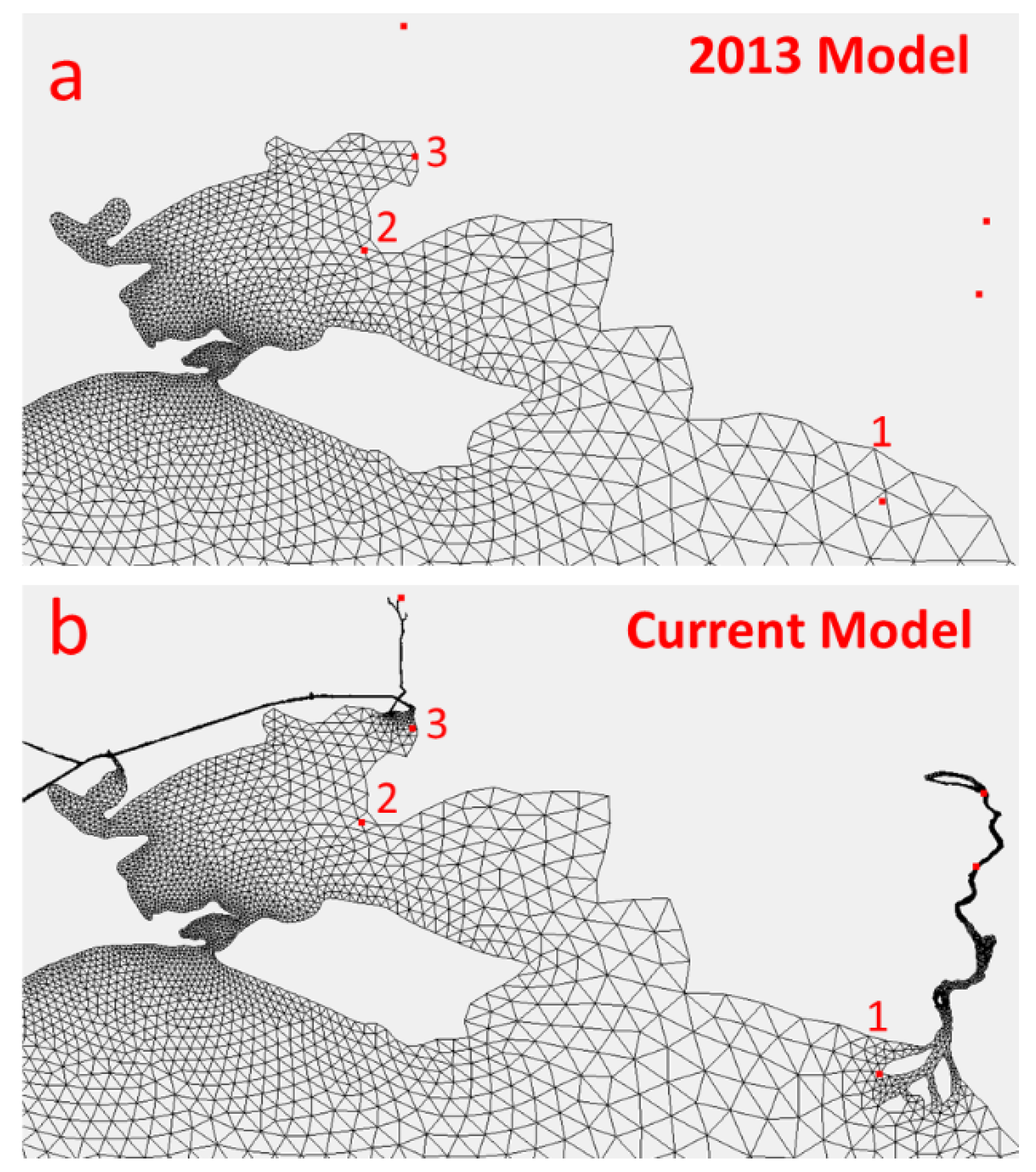
3.5. Comparisons of the Updated Tidal Model with the Previous Tidal Model

The major improvement of the model update comes from the work including: (1) model grid extension to include new tide stations; (2) the incorporation of the best available data (shoreline, bathymetry, and tide stations); (3) the implementation of a better version of the ADCIRC model; (4) the implementation of the most recently developed tidal database EC2015; and (5) the implementation of the SVU statistical interpolation method. In this section, we will compare the statistical values of the ADCIRC model errors between the updated tidal model and the previous tidal model to understand the overall model improvement.

First, let us focus on the area with the major model grid extension in the western LA region, as shown in Figure 16. Three tide stations in this region were included in both the current and previous model domains. We used the current CO-OPS data of observed tidal datums and modeled tidal datums from the current and previous tidal models to analyze how much the updated tidal model improves the modeled tidal datums in this model area.

Table 2. The statistical values of the model errors from the current and previous tidal models (in meters).

Tide Station	MHHW (M-O)	MHW (M-O)	MLW (M-O)	MLLW (M-O)
1	−0.011 (0.009)	0.009 (0.032)	−0.093 (−0.022)	−0.078 (−0.090)
2	−0.057 (−0.063)	−0.029 (−0.046)	−0.001 (0.013)	0.050 (0.049)
3	−0.025 (−0.030)	−0.016 (−0.030)	−0.012 (0.005)	0.037 (0.038)
Mean |Error|	0.031 (0.034)	0.018 (0.036)	0.035 (0.013)	0.055 (0.059)

Note: “M” represents “Model”, and “O” represents “Observation”. The values outside the parentheses are from the current tidal model. The values inside the parentheses are from the previous tidal model. “Mean |Error|” refers to “the average of the absolute model errors” over the three tide stations. The values in bold indicate that the model errors in the previous tidal model are greater than in the current tidal model.

lists the statistical values of the model errors from the current and previous tidal models. The values outside the parentheses are from the current tidal model, while the values inside the parentheses are from the previous tidal model. The values in bold indicate that the model errors in the previous tidal model are greater than those in the current model. Based on Table 2, the updated model improved the modeled MHW at all the three stations, improved the modeled MHHW/MLLW at two of the three tide stations, and improved MLW only at Station 2. That is, the updated model outperformed the previous model in simulating MHHW/MHW/MLLW in this model area. The mean absolute errors indicate that statistically the updated model outperformed the previous model in the modeled MHW the most, MLLW the second most, and MHHW the third most, but underperformed the previous model in the modeled MLW.

Next, a similar statistical analysis was conducted in the entire model domain at all the 69 tide stations which were included in both the current and previous model domains; that is, the six out of the 75 tide stations that were included in the current model domain by model grid extension but were not included in the previous tidal model domain, were excluded in the statistical analysis. We obtained similar results as in the abovementioned analysis over the three stations. The updated tidal model outperformed the previous tidal model in simulating MHHW (39 out of the 69 tide stations), MHW (36 out of the 69 tide stations), and MLLW (38 out of the 69 tide stations), but underperformed the previous model in simulating MLW (54 out of the 69 tide stations). The difference of the mean absolute errors over the 69 stations between the previous tidal model and the current tidal model (the mean absolute errors of the previous tidal model minus the mean absolute errors of the current tidal model) is: 0.002 m (MHHW), 0.003 m (MHW), −0.013 m (MLW), and 0.003 m (MLLW). This indicates that statistically, the updated tidal model outperformed the previous tidal model in simulating MHHW/MHW/MLLW, but underperformed the previous tidal model in simulating MLW over the entire model domain.

4. Summary

This paper introduces the procedures and the methodologies used in updating the tidal model and the modeled tidal datums in the TX and western LA coastal waters, presents and discusses the obtained results, shares effective techniques used for improving the hydrodynamic model performance and lessons learned in the model assessment, and statistically analyzes the model improvement in simulating the tidal datums.

The updated tidal model statistically outperformed the previous tidal model in most cases. The SVU statistical interpolation method interpolated the modeled tidal datums to within a user-defined error (0.01 m in this work), which was demonstrated to reduce the model biases and model errors in comparison with the previous deterministic approach (TCARI) based on the previous study [13]. The statistical interpolation also produced the spatially varying uncertainty field for each interpolated tidal datum, which offers the spatial characteristics of the uncertainty field, much better than the previous single-value model uncertainty over an entire VDatum model domain. The upgraded non-tidal polygons enhanced the quality of the VDatum marine grid population and thus the final tidal datum products.

The accuracy of a tide station’s coordinates was shown to significantly influence the outcome and thus the quality of the model assessment, which should be an important lesson for the modeling community in general.

References

1. NOAA/NOS VDatum Website. Available online: https://vdatum.noaa.gov/ (accessed on 6 February 2019).
2. Gill, S.; Schultz, J. Tidal Datums and Their Applications; NOAA Special Publication NOS CO-OPS 1: Silver Spring, MD, USA, 2000. Available online: http://www.tidesandcurrents.noaa.gov/publications/tidal_datums_and_their_applications.pdf (accessed on 6 February 2019).
3. Myers, E.P. Review of progress on VDatum, a vertical datum transformation tool. In Proceedings of the OCEANS 2005 MTS/IEEE, Washington, DC, USA, 17–23 September 2005; pp. 974–980. [Google Scholar]
4. Myers, E.; Hess, K.; Yang, Z.; Xu, J.; Wong, A.; Doyle, D.; Woolard, J.; White, S.; Le, B.; Gill, S.; et al. VDatum and strategies for national coverage. In Proceedings of the OCEANS 2007, Vancouver, BC, Canada, 29 September–4 October 2007; pp. 1–8. [Google Scholar]
5. Hess, K.; Kenny, K.; Myers, E. Standard Procedures to Develop and Support NOAA’s Vertical Datum Transformation Tool, VDATUM (Version 2010.08.03); NOAA NOS Technical Report; NOAA NOS: Silver Spring, MD, USA, 2012.
6. Xu, J.; Myers, E. Modeling tidal dynamics and tidal datums along the coasts of Texas and Western Louisiana. In Proceedings of the 11th International Conference on Estuarine and Coastal Modeling, Seattle, WA, USA, 4–6 November 2009. [Google Scholar]
7. Xu, J.; Myers, E.P.; Jeong, I.; White, S.A. VDatum for the Coastal Waters of Texas and Western Louisiana: Tidal DAtums and Topography of the Sea Surface; NOAA: Silver Spring, MD, USA, 2013.
8. ADCIRC Users Manuals. Available online: https://adcirc.org/home/documentation/users-manuals-compile-options-faqs-wiki/ (accessed on 6 February 2019).
9. Luettich, R.A., Jr.; Westerink, J.J.; Scheffner, N.W. ADCIRC: An Advanced Three-Dimensional Circulation Model for Shelves, Coasts, and Estuaries. Report 1. Theory and Methodology of ADCIRC-2DDI and ADCIRC-3DL; Coastal Engineering Research Center: Vicksburg, MS, USA, 1992. [Google Scholar]
10. Westerink, J.J.; Luettich, R., Jr.; Scheffner, N. ADCIRC: An Advanced Three-Dimensional Circulation Model for Shelves, Coasts, and Estuaries. Report 3. Development of a Tidal Constituent Database for the Western North Atlantic and Gulf of Mexico; Coastal Engineering Research Center: Vicksburg, MS, USA, 1993; Available online: https://apps.dtic.mil/dtic/tr/fulltext/u2/a268685.pdf (accessed on 6 February 2019).
11. Westerink, J.; Luettich, R., Jr.; Blain, C.; Scheffner, N.W. ADCIRC: An Advanced Three-Dimensional Circulation Model for Shelves, Coasts, and Estuaries. Report 2. User’s Manual for ADCIRC-2DDI; Army Engineer Waterways Experiment Station: Vicksburg, MS, USA, 1994; Available online: file:///C:/Users/Wei.Wu/Downloads/ADCIRC_An_Advanced_Three-Dimensional_Circulation_M%20(1).pdf (accessed on 6 February 2019).
12. National Hurricane Center Tropical Cyclone Report. Available online: https://www.nhc.noaa.gov/data/tcr/ (accessed on 6 February 2019).
13. Shi, L.; Myers, E. Statistical Interpolation of Tidal Datums and Computation of Its Associated Spatially Varying Uncertainty. J. Mar. Sci. Eng. 2016, 4, 64. [Google Scholar] [CrossRef]
14. Gill, S.; Michalski, M. Classification of a Water Level Station as Non-Tidal; NOAA SOP # 7.3.A.1; NOAA: Silver Spring, MD, USA, 2016.
15. Mao, M.; Xia, M. Dynamics of wave–current–surge interactions in Lake Michigan: A model comparison. Ocean Model. 2017, 110, 1–20. [Google Scholar] [CrossRef]
16. Akbar, M.K.; Luettich, R.A.; Fleming, J.G.; Aliabadi, S.K. CaMEL and ADCIRC Storm Surge Models—A Comparative Study. J. Mar. Sci. Eng. 2017, 5, 35. [Google Scholar] [CrossRef]
17. Vinogradov, S.; Myers, E.; Funakoshi, Y.; Moghimi, S.; Calzada-Morrero, J. Real-Time Storm Surge Forecasting Systems Research, Design, and Development. In Proceedings of the 98th American Meteorological Society Annual Meeting, Austin, TX, USA, 7–11 January 2018; Available online: https://ams.confex.com/ams/98Annual/webprogram/Paper327250.html (accessed on 6 February 2019).
18. Funakoshi, Y.; Feyen, J.C.; Aikman, F.; van der Westhuysen, A.J.; Tolman, H.L. The Extratropical Surge and Tide Operational Forecast System (ESTOFS) Atlantic Implementation and Skill Assessment; NOAA Technical Report NOS CS 32; NOAA: Silver Spring, MD, USA, 2013; 147p.
19. Xu, J.; Feyen, J.C. The Extra Tropical Surge and Tide Operational Forecast System for the Eastern North Pacific Ocean (ESTOFS-Pacific): Development and Skill Assessment; NOAA Technical Report NOS CS 36; NOAA: Silver Spring, MD, USA, 2016; 153p.
20. ADCIRC EC2015 Tidal Database. Available online: http://adcirc.org/products/adcirc-tidal-databases/ (accessed on 9 February 2019).
21. Szpilka, C.; Dresback, K.; Kolar, R.; Feyen, J.; Wang, J. Improvements for the Western North Atlantic, Caribbean and Gulf of Mexico ADCIRC Tidal Database (EC2015). J. Mar. Sci. Eng. 2016, 4, 72. Available online: https://doi.org/10.3390/jmse4040072 (accessed on 6 February 2019). [CrossRef]
22. Mukai, A.Y.; Westerink, J.J.; Luettich, R.A., Jr.; Mark, D. Eastcoast 2001, a Tidal Constituent Database for Western North Atlantic, Gulf of Mexico, and Caribbean Sea; Engineer Research and Development Center Vicksburg Ms Coastal and Hydraulicslab: Technical Report, ERDC/CHL TR-02-24; US Army Engineer Research and Development Center, Coastal and Hydraulics Laboratory: Vicksburg, MS, USA, 2002; 201p, Available online: https://coast.nd.edu/reports_papers/2001-Mukai-TR-02-24.pdf (accessed on 6 February 2019).
23. Egbert, G.D.; Svetlana, Y.E. The OSU TOPEX/Poseidon Global Inverse Solution TPXO. Available online: http://volkov.oce.orst.edu/tides/global.html (accessed on 6 February 2019).
24. Egbert, G.D.; Svetlana, Y.E. OTIS Regional Tidal Solutions. Available online: http://volkov.oce.orst.edu/tides/Mex.html (accessed on 6 February 2019).
25. SMS—The Complete Surface-water Solution. Available online: https://www.aquaveo.com/software/sms-surface-water-modeling-system-introduction (accessed on 6 February 2019).
26. NOAA Shoreline Website—NOAA Continually Updated Shoreline Product (CUSP). Available online: https://www.ngs.noaa.gov/CUSP/ (accessed on 6 February 2019).