Article

Modelling Behaviour of the Salt Wedge in the Fraser River and Its Relationship with Climate and Man-Made Changes

by
Albert Tsz Yeung Leung
1,*,
Jim Stronach
1 and
Jordan Matthieu
2
1
Tetra Tech Canada Inc., Water and Marine Engineering Group, 1000-10th Floor 885 Dunsmuir Street, Vancouver, BC V6C 1N5, Canada
2
WSP, Coastal, Ports and Maritime Engineering, 1600-René-Lévesque O., 16e étage, Montreal, QC H3H 1P9, Canada
*
Author to whom correspondence should be addressed.
J. Mar. Sci. Eng. 2018, 6(4), 130; https://doi.org/10.3390/jmse6040130
Submission received: 20 September 2018 / Revised: 3 November 2018 / Accepted: 3 November 2018 / Published: 6 November 2018

Abstract

:
Agriculture is an important industry in the Province of British Columbia, especially in the Lower Mainland where fertile land in the Fraser River Delta combined with the enormous water resources of the Fraser River Estuary support extensive commercial agriculture, notably berry farming. However, where freshwater from inland meets saltwater from the Strait of Georgia, natural and man-made changes in conditions such as mean sea level, river discharge, and river geometry in the Fraser River Estuary could disrupt the existing balance and pose potential challenges to maintenance of the health of the farming industry. One of these challenges is the anticipated decrease in availability of sufficient freshwater from the river for irrigation purposes. The main driver for this challenge is climate change, which leads to sea level rise and to reductions in river flow at key times of the year. Dredging the navigational channel to allow bigger and deeper vessels in the river may also affect the availability of fresh water for irrigation. In this study, the salinity in the river was simulated using H3D, a proprietary three-dimensional hydrodynamic numerical model which computes the three components of velocity (u,v,w) in three dimensions (x,y,z) on a curvilinear grid developed specially for Fraser River, as well as scalar fields such as salinity and temperature. The results indicate various levels of impact to the salinity in the river and adaptive measures must be established to maintain the long-term viability of the industry. This study found that sea level rise and changes in river discharge would have a larger impact on the availability of fresh water than would channel deepening at the present sea water level. In a low river discharge regime, the impact from sea level change is more significant than in the high river discharge regime. On the other hand, the influence from changes in river discharge on withdrawal appears to increase when water level is lowered. Dredging the channel to accommodate larger vessels with deeper draft would further affect the salinity and shorten the withdrawal window; the effect of channel deepening becomes more pronounced in the lower flow period.

1. Introduction

Many of the largest economies in the world are located near or in a river estuary where saline water from the ocean meets the freshwater draining from inland: The Hudson River in New York, the Mississippi River in New Orleans, the Buffalo Bayou in Houston, the Yellow River in Shanghai, and the Pearl River in Hong Kong, just to name a few. These are not coincident, because an estuary often is of critical commercial value to nearby areas; and altogether, estuaries serve to contribute not only to human welfare and value to the world’s economy, but also provide essential ecosystem services such as food production and recycling of nutrients [1]. Among the many commercial functions it can serve, an estuary can be a conduit for transport of goods and products, and is very often an important water resource for domestic, industrial, and agricultural use. These economic benefits brought forth by an estuary are of course in addition to the environmental benefits resulting from a highly diverse ecosystem that an estuary usually sustains due to its unique hydrodynamic and geomorphologic settings.
The hydrodynamic behavior and salinity of an estuary is sensitive to climate change that could potentially affect sea level and the hydrological characteristics that dictate the amount of watershed runoff. This delicate balance is further complicated by future changes in river management such as channel deepening in order to allow navigation by larger vessels in the estuary. Understanding the complicated interaction between changes in sea level and runoff as well as bathymetry of the river and their impacts on the salinity in the river is therefore essential for developing proper and timely strategies to ensure resiliency of coastal areas against natural and anthropogenic changes in the future.
The hydrodynamics of the Fraser River estuary has been extensively studied in the past: Stronach et al. [2,3], and Halverson and Pawlowicz [4,5] studied and described the river plume dynamics of the Fraser River outflow into the Strait of Georgia. Halverson and Pawlowicz [6], Kostaschuk and Atwood [7], and Ward [8] particularly investigated the river flow and tidal forcing in the Fraser River estuary and their effects on salinity. Yin et al. [9] studied the biological significance of the salt wedge dynamics in the Fraser River estuary. Neilson-Welch and Smith [10] observed and described the effects of the upstream intrusion of saltwater.
There is limited, if any, published literature regarding specifically the effects of sea level rise (SLR) and changes in river discharge and river geometry on salinity distribution in the Fraser River, but similar studies were undertaken in other parts of the world: Krvavica et al. [11] studied the salt wedge in the Rjecina River Estuary in Croatia using a finite volume model; Funahashi et al. [12] developed a numerical model using Delft3DFlow to investigate the response of the salt wedge and salinity distribution in the river to the short-term changes in sea level and river discharge in the Yura Estuary in Japan; and Shaha et al. [13] studied the saltwater intrusion in Sumjin River Estuary in South Korea using the Finite Volume Community Ocean Model (FVCOM) and related intrusion length and river discharge by a power law.

2. Study Site

The Fraser River estuary, located south of Vancouver, is an important part of the economy in the Province of British Columbia (BC), Canada [14]. The Fraser River delta is fertile and, as such, the agricultural industry in the region is thriving, with a noticeable increase in the farmland area in the late 20th and early 21st centuries [15]. There is potential for significant growth in terms of agricultural production, provided that additional water can be withdrawn from the river for irrigation [16]. The low-salinity water withdrawn from the river for irrigation is therefore of critical importance to the continued health of the farmland and its agricultural products.
The Fraser River is connected at its downstream boundary to the Strait of Georgia (SOG), which in turn is connected to the open Pacific Ocean through the connections at Juan de Fuca Strait to the south and Johnstone Strait to the north. Therefore, water level in the SOG and the Fraser River is subject to tidal fluctuations. Figure 1 below illustrates the study location as well as the geographic and hydrographic relations between the Fraser River, the SOG, and the Pacific Ocean.
The tidal range in the Fraser River is variable, depending not only on the tidal fluctuation in the SOG, but also on distance upstream from the river mouth and on river discharge. At the river mouth, the tide is mixed, mainly semi-diurnal, and exhibits a clear alternating neap tide and spring tide pattern. The higher high water level is 2.0 m above mean sea level, which in turn is 3.1 m above chart datum, resulting in a tidal range of 5.1 m. This tidal effect, though diminishing in an upstream direction, can reach as far upstream as Mission, approximately 84 km from the river mouth.
The stratification in the SOG and the Fraser River is due to the presence of saltwater from the Pacific Ocean and freshwater from river runoff. The interaction of the freshwater and saltwater masses in the Fraser River Estuary gives rise to the formation of a salt-wedge, which intrudes from the SOG into the river in an upstream direction. While the salt wedge occupies the part of the water column from the bottom to a certain depth, the fresh river water, upon meeting the salt wedge, travels downstream on top of the salt-wedge. The extent of the intrusion varies depending on the river discharge and water level in the SOG: while the position and salinity of the salt-wedge displays an intra-day pattern in response to the semi-diurnal tidal fluctuation in the Strait, the mean daily position of the salt-wedge moves upstream and downstream in response to the changes in river discharge. The salinity in the river has a strong correlation with the salt-wedge intrusion and thus displays similar fluctuation patterns.

3. Materials and Methods

The core component of the study is the numerical simulation of the salt wedge in the Fraser River, the largest river in BC, which drains into the SOG in the Salish Sea, under a range of climate change, river flow, and river configuration scenarios. A numerical model of the Fraser River, based on the modelling platform H3D developed by Tetra Tech, has been implemented and calibrated for present conditions; however, the fundamental processes: bottom friction, vertical mixing, salt wedge migration under tidal influence, are all intrinsic processes, i.e., their formulation depends only on the specific flow and water level conditions imposed by external influences. In other words, the model is totally objective with respect to evaluating climate change. Thus, the model does not require modification for this work. However, it is important to select and properly quantify climate change scenario inputs for modelling.

3.1. Three-Dimensional Hydrodynamic Numerical Model: H3D

H3D is an implementation of the numerical model developed by Backhaus [17,18], which has had numerous applications to the European continental shelf [19,20], Arctic waters [21,22], and deep estuarine waters [23]. Locally, H3D has been used to model the temperature structure of Okanagan Lake [24], the transport of scalar contaminants in Okanagan Lake [25], sediment movement and scour/deposition in the Fraser River, circulation and wave propagation in Seymour and Capilano dams, and salinity movement in the lower Fraser River. H3D forms the basis of the model developed by Saucier and co-workers for the Gulf of St. Lawrence [26], and has been applied to the Gulf of Mexico [27].

3.1.1. Theoretical Basis

H3D is a three-dimensional time-stepping numerical model which computes the three components of velocity (u,v,w) on a structured grid in three dimensions (x,y,z), as well as scalar fields such as salinity, temperature, and contaminant concentrations. The model uses the Arakawa C-grid in space [28], and uses a two level semi-implicit scheme in the time domain. The Arakawa C-grid evaluates velocity vector components at the centres of the grid faces (i.e., u-component velocities are evaluated at the centres of the east and west grid faces, v-component velocities on the north and south grid faces, and w-component velocities on the top and bottom grid faces, while scalar quantities are calculated in the grid centres). The size of the model time step varies depending on the horizontal grid size and velocity at each of the grid cells: the model, at each time step and each grid cell, calculates the numerically-stable time step based on the u-, v-, and w-components of the velocity and the x-, y-, and z-dimensions of the grid cell; the model then updates the time step by choosing the largest time step that will satisfy the numerical stability for all grid cells. Details with respect to the derivation of the model are provided in Appendix A.

3.1.2. Grid Geometry

In the horizontal, the grid cells can be either rectilinear or orthogonal curvilinear, depending on the physical characteristics of the water body of interest. Details regarding the horizontal resolution and configuration of the models are described in Section 3.2. In the vertical, the levels near the surface are typically closely spaced to assist with resolving near-surface dynamics. Figure 2 shows a typical grid mesh utilized for the H3D model.
In addition, the model is capable of dealing with relatively large excursions in overall water level as the water level rises and falls in response to varying inflows and outflows, by allowing the number of near-surface layers to change as the water level varies. That is, as water levels rise in a particular cell, successive layers above the original layer are turned on and become part of the computational mesh. Similarly, as water levels fall, layers are turned off. This procedure has proven to be quite robust, and allows for any reasonable vertical resolution in near-surface waters. When modelling thin river plumes in areas of large tidal range, the variable number of layers approach allows for much better control over vertical resolution than does the σ-coordinate method.
In addition to tides, the model is able to capture the important response, in terms of enhanced currents and vertical mixing, to wind-driven events. This is achieved by applying wind stress to each surface grid point on each time step. Vertical mixing in the model then re-distributes this horizontal momentum throughout the water column. Similarly, heat flux through the water surface is re-distributed by turbulence and currents in temperature simulations.

3.1.3. Turbulent Closure

Turbulence modelling is important in determining the correct distribution of velocity and scalars in the model. The diffusion coefficients for momentum (AH and AV) and scalars (NH and NV) at each computational cell are dependent on the level of turbulence at that point. H3D uses a shear-dependent turbulence formulation in the horizontal presented by Smagorinsky [29]. The basic form is:
A H = A H 0 d x d y ( d u d x ) 2 + ( d v d y ) 2 + 1 2 ( v x + u y ) 2  
where the parameter AH0 is a dimensionless tuning variable, and experience has shown it to lie in the range of 0.25 to 0.45 for most water bodies such as rivers, lakes and estuaries.
A shear and stratification dependent formulation, the Level 2 model of Mellor and Yamada [30], is used for the vertical eddy diffusivity. The basic theory for the vertical viscosity formulation is taken from an early paper by Mellor and Durbin [31]. The evaluation of length scale is based on a methodology presented by Mellor and Yamada [30].
For scalars, both horizontal and vertical eddy diffusivity are taken to be similar to their eddy viscosity counterparts, but scaled by a fixed ratio from the eddy viscosity values. Different ratios are used for the horizontal and vertical diffusivities. If data is available for calibration, these ratios can be adjusted based on comparisons between modelled and observed data. Otherwise, standard values based on experience with similar previously modelled water bodies are used. In a recent reservoir simulation with good calibration data, the ratio of vertical eddy diffusivity to vertical eddy viscosity was 0.75 and the ratio between horizontal eddy diffusivity and horizontal eddy viscosity was 1.0.

3.1.4. Scalar Transport

The scalar transport equation implements a form of the flux-corrected algorithm presented by Zalesak [32], in which all fluxes through the sides of each computational cell are first calculated using a second-order method. Although generally more accurate than a first order method, second order flux calculations can sometimes lead to unwanted high frequency oscillations in the numerical solution. To determine if such a situation is developing, the model examines each cell to see if the computed second order flux would cause a local minimum or maximum to develop. If so, then all fluxes into or out of that cell are replaced by first order fluxes, and the calculation is completed. As noted, the method is not a strict implementation of the Zalesak method, but is much faster and achieves very good performance with respect to propagation of a Gaussian distribution through a computational mesh. It does not propagate box-car distributions as well as the full Zalesak method, but achieves realistic simulations of the advection of scalars in lakes, rivers, and estuaries, which is the goal of the model. This scheme as implemented is thus a good tradeoff between precision and execution time, important since in many situations, where more than one scalar is involved, the transport-diffusion algorithm can take up more than half the execution time.

3.1.5. Heat Flux at the Air–Water Interface

The contribution of heat flux to the evolution of the water temperature (T) field is schematized in H3D as:
T t = Δ F ρ C P h  
where Δ F is the net heat flux per unit area retained in a particular layer, ρ is the density of water, Cp is the heat capacity of water, and h is the layer thickness. Heat flux at the air–water interface incorporates the following terms:
  • Fin: incident short wave radiation. Generally, this is not known from direct observations. Instead, it is estimated from the cloud cover and opacity observations at nearby stations, a theoretical calculation of radiation at the top of the atmosphere based on the geometry of the earth/sun system, and an empirical adjustment based on radiation measurements at Vancouver International Airport for the period 1974–1977. This procedure has worked well for many water bodies, notably Okanagan Lake and the waters of the north coast of British Columbia, in terms of allowing H3D to reproduce the observed temperature distributions in space and time. Values for albedo as a function of solar height are taken from Kondratyev [33].
  • Fback: net long wave radiation. This is calculated according to Gill [34], involving the usual fourth power dependence on temperature, a factor of 0.985 to allow for the non-black body behaviour of the ocean, a factor depending on vapor pressure to allow for losses due to back radiation from moisture in the air, and a factor representing backscatter from clouds.
  • FL and FS: Latent heat flux (FL) is the heat carried away by the process of evaporation of water. Sensible heat flux (FS) is driven by the air-water temperature difference and is similar to conduction, but assisted by turbulence in the air. Latent and sensible heat fluxes are described by:
    Q L = 1 . 32 e 2 L U a ( q o b s q s a t ) F l ,   and
    Q S = 1 . 46 e 3 ρ a i r c p U a ( T a i r T w a t e r ) F s ,
    where qobs and qsat are the observed and saturated specific humidities, Tair and Twater are the air and water temperatures, L is the latent heat of evaporation of water, and Cp is the heat capacity of water, Ua is wind speed, Fl and Fs are latent and sensible factors, which are the scaling factors introduced to account for local factors, and can be adjusted, when needed, to achieve better calibration of the model. Typically, the only adjustment is that sensible factor is doubled when the air temperature is less than the water or ice surface temperature to account for increased turbulence in an unstable air column.
As light passes through the water column it is absorbed and the absorbed energy is a component of the energy balance that drives water temperature. H3D assumes that light attenuation follows an exponential decay law:
E ( z ) = E ( z 0 ) e k ( z z 0 ) ,
where E(z) is the insolation at a distance, z, below the water surface, and E(z0) is the incident insolation at the water surface. The model computes the energy at the top and bottom of each layer and the difference is applied to the general heat equation in that layer. The extinction coefficient (k) is related to the Secchi depth (Ds) by:
k = 2 . 1 D s .
Temperature is treated like any other scalar as far as advection and diffusion are concerned.

3.2. Model Implementation

A study of the details of the hydrodynamics of the Fraser River requires model nesting to better resolve small scale processes at and near locations of interest. The model used for this study operates in a triple-nested configuration, shown in Figure 3.
The investigation of the behaviour of the salt wedge was undertaken with a nominally 50-m resolution curvilinear model that spans the lower 41 km of the Fraser River, from Sand Heads to the Port Mann Bridge. The model uses 50-m resolution in the along-channel direction, and 20-m in the cross-channel direction. This 50-m resolution model is in turn embedded within a nominally 1-km resolution rectilinear model of the entire SOG. The vertical resolution of the models varies with depth and is 1 m for the top 10 m, 2 m for depth of 10–16 m, 3 m for 16–25 m, 10 m for 25–55 m, 25 m for 55–105 m, 50 m for 105–305 m, and 100 m for 305–505 m. The higher vertical resolution near the top is necessary to resolve the complex hydrodynamic processes and the sharp salinity gradient at the interface of the salt wedge.
Both models simulate tidal, wind-driven, and density-driven currents. Water level, velocity components, and any scalar quantities (i.e., temperature and salinity) output from the coarse grid model are passed on along the boundaries of the fine grid model and used to drive the finer-scale implementation of H3D. The fine-grid implementation provides the details of the effect of small-scale spatial variability in shorelines, depths and structures such as the tunnel cover.
The 1-km SOG model, driven by wind, temperature, and salinity as well as tidal conditions along its open boundaries bordering the northern entrance to the SOG and the western entrances to Juan de Fuca Strait, includes a coarse representation of the Fraser River, extending 41 km upstream from the river mouth at Sand Heads to the Port Mann Bridge. At that location, upstream of all salt wedge penetration, the model is dynamically coupled to a one-dimensional (1-D) model of the Fraser River, extending to Hope, which is located approximately 130 km upstream from the river mouth and is free of any tidal effects. The model coupling is two-way as the SOG model provides water level to the downstream boundary of the 1-D model, which in turn calculates the flow conditions at that same boundary given the discharge rate at the upstream boundary of the 1-D model at Hope. The initial and boundary conditions for temperature and salinity are provided by Crean and Ages [35], which documented a comprehensive temperature and salinity measurement campaign in the SOG and Juan de Fuca Strait. Tidal conditions are also specified along the open boundaries.
The 50-m lower Fraser River model is driven at its upstream end by flow boundary conditions provided by a separate, dynamically coupled 1-D Fraser River model. At the downstream end, water levels as well as temperature and salinity profiles are obtained from the 1-km SOG model, spatially interpolated from those cells of the 1-km SOG model that correspond to the boundaries of the 50-m Fraser River model.
Table 1 below summarizes the modelling sequence (Seq. #), the initial conditions and boundary conditions utilized for the modelling study:

3.3. Validation of the Nested Model

The models were initialized on 1 January 2011 and run through the 6-month long harvest season period, between August and December, when the ability to withdraw freshwater from the river is crucial. The year 2011 was chosen for the model validation as this is the year for which bank-to-bank bathymetric survey data collected in the Fraser River estuary is available: the model bathymetry was constructed using this 2011 data set; the Fraser River flow rate in 2011 was used to drive the upstream boundary of the river model, and the tidal conditions in 2011 were specified along the open boundaries in the SOG model. The flow rate at the upstream boundary of the model is the combination of the flow rate at Hope and the estimated runoffs that report to the river downstream of Hope and upstream of the Port Mann Bridge. Figure 4 shows the observed river flow rate at Hope in the year 2011 [36].
The model was validated against water levels recorded at New Westminster, which is located 34 km upstream from the river mouth, and against conductivity data collected by a sensor mounted at 2 m depth from a floating platform installed at an irrigation intake near 8081 River Road, Delta, approximately 24 km upstream from the river mouth. Figure 5 shows a comparison of observed and modelled conductivity values at the water intake (location shown in Figure 6) at a depth of 2 m from 3rd to 23rd November 2011, when the leading edge of the salt wedge passed upstream and downstream through the sensor location and the conductivity signal ranged between zero and the maximum value that the sensor could record, 5500 μS/cm. Comparison of the observed and modelled results for months other than November would have been undertaken if not for the lack of reliable, continual conductivity measurement at other locations in the river (identified as data gap in Section 5.4). Also included in the figure are observed and modelled water levels for the same period. Black lines show modelled values and red lines show observed values. Since the conductivity sensor cuts off at 5500 μS/cm, the model results were similarly cut-off to facilitate comparison.
The days on which the observed conductivity is considerably lower than the modelled correspond almost perfectly with the days with rainfall in the catchment downstream of the Harrison River exceeding 15 mm/day: 7, 10–12, 17, 21–22 November. A rainfall of 15 mm/day corresponds, approximately, to an additional flow in the Fraser River of up to 1000 m3/s, depending on the hydrological processes controlling how this additional water reports to the river. This additional fresh water would undoubtedly lead to significant reduction in conductivity in the river during rainfall events.
Otherwise, the model is, in general, able to re-create the timing and the trend of the conductivity signal, as well as partially the strength of the signal (Correlation Coefficient (R) = 0.53; Root-Mean-Square-Error (RMSE) = 1571 μS/cm or 1.37 ppt), in both the daily time scale and multi-day time scale. However, there are some disagreements in the conductivity values and the exact timing of the fluctuations at the water intake. For example, the model almost always predicts an elevation of conductivity during high tides when river flow is comparatively slower and water level in the river higher (for example, on 7 November); however, the sensor at the intake did not always detect such a conductivity signal.
The complexity in the behaviour of the conductivity signal can be partly understood by considering Figure 6, showing the map of salinity at the 2-m depth, on 11 November 2011, at 7 a.m., where the modelled result appears to deviate the most from the observed value. The vectors indicate the direction and strength of the water movement at the 2-m depth. It can be seen that there is a high degree of spatial variability in the salinity field in the vicinity of the intake. Salinity can vary from 3.5 ppt (4500 μS/cm) to more than 5.0 ppt (6500 μS/cm) near the intake in a matter of metres. Further analysis of model output demonstrates that there are two mechanisms for saline water to intrude onto the relatively shallow shelf on which the intake is located: either a selective withdrawal process, whereby saltier water is drawn up onto the bench from the adjacent deeper water (on both ebb and flood), or a process whereby the toe of the salt wedge rises to the surface upstream of the bench and then falls back partially onto the bench on the ebb tide.
Besides direct comparison of observed and modelled salinity, this model validation can be considered from the perspective of water availability, which describes the onset and offset of salinity intrusion at the water intake and the time window within which river water can be safely withdrawn under the criterion salinity value of 0.35 ppt or conductivity of 400 μS/cm. Figure 7 below compares the observed and modelled number of available hours per running 24 h. The red line represents the observation and the black line represents the model results. Only a short period of record is presented to facilitate visual comparison.
The model, even though more conservative in general, was able to predict the overall trend in availability (R = 0.60; RMSE = 5.9 h). The numerical model predicts that water suitable for irrigation in November is available for 10 h per day whereas observations indicate that suitable water is available, on average, 14 h per day.

3.4. Study Methodology

The effects of changes in environmental (sea level rise and river flow changes as a result of climate change) and anthropogenic (channel deepening) conditions on the behaviour of the salt wedge and salinity distribution in the Fraser River were the main focus of this study. Climate change scenarios were chosen based on the Fraser River flow rate predicted by a Global Climate Model (GCM), selected for its demonstrated ability to closely hindcast the historical flow in the river (Section 3.1), during the irrigation period between August and October. Several sea level rise scenarios were evaluated in this study and ultimately the sea level rises appropriate for the time horizon in year 2050 and year 2100 were used (Section 3.2). Given the projected economic growth of the region, there could be a need to allow deeper draft vessels to navigate the Fraser River to provide sufficient capacity. The dredge depth which allows for most Panamax and derivative vessel classes to navigate in the Fraser River was evaluated in the model study (Section 3.3).

3.4.1. Selecting Climate Scenario and Global Climate Model for Projection of the Fraser River Hydrograph

Three climate scenarios were considered in this study. Denoted A1B, B1, and A2, these scenarios, according to the Fourth Assessment Report (AR4) published by the Intergovernmental Panel on Climate Change (IPCC) in 2007 [37], relate to how different types of societal behaviour lead to different levels of greenhouse gas emissions and subsequent climate change. The emission scenarios based on AR4 were chosen for this study because the projected Fraser River hydrograph derived by the Pacific Climate Institute Consortium, or PCIC, is based on these scenarios. Table 2 summarizes the characteristics of these climate scenarios.
The selection process of a suitable projected Fraser River hydrograph involved evaluation of a set of eight GCMs, driven by the aforementioned three climate scenarios, each representing relatively low, medium, and high atmospheric greenhouse gas concentration increases in the future. These eight GCMs were selected for best matching the downscaled results of these GCMs with the historical data in the 1950–2005 period in western Canada. This method produced an ensemble of all raw projections for temperature and precipitation at a global-scale. The GCMs provided these projections in the form of average temperature and precipitation changes in grid cells, where individual grid cells are approximately 300 km × 300 km (~90,000 sq. km or 9 million hectares) in size. These grid cell values were then statistically downscaled to a watershed-scale resolution of approximately 6 km × 6 km grid cells using a technique called Bias Corrected Spatial Disaggregation before being fed into the Variable Infiltration Capacity (VIC) hydrologic model for estimating streamflow. This approach was discussed in detail in Werner [38] and Schnorbus et al. [39].
An ensemble average was calculated based on the daily flow results derived from these eight different GCMs, each appropriately downscaled to produce Fraser River flows at Hope, and averaged to produce daily flows over an indicated time period. Figure 8 illustrates the ensemble average of the daily Fraser River flow rate under a range of climate change scenarios and different time horizon (present: 2000–2014, short-to mid-term horizon: 2016–2050; long-term horizon: 2051–2098). The data results were published by PCIC [40].
The predicted average flow rate in the irrigation period, under a range of climate change scenarios in 2050 (ranging between 1142 m3/s and 2352 m3/s) and 2098 (ranging between 730 m3/s and 1540 m3/s), is less than the existing rate (ranging between 1204 m3/s and 3025 m3/s).
The climate scenario, A1B, was eventually chosen for the projected Fraser River flow in this modelling study, not only because it represents a scenario which reflects the likely evolution of human society in the next century, but also it projects a lower river discharge and likely higher salinity during the irrigation period. As the original objective of this study was to assist engineers and planners to establish appropriate adaptive measures to maximize freshwater withdrawal for irrigation, the model results based on the A1B scenario would provide the relevant parties conservative estimates of the withdrawal window such that sufficient resources can be planned and assigned to mitigate the potential impact.
With regard to selecting between the various GCMs, Figure 9 below shows the comparison of the Fraser River hydrograph at Hope between the observed and modelled values derived from the 8 GCM models for calendar years from 1998 to 2004. The level of agreement and disagreement varies both between models, and from month to month and year to year.
This figure indicates that the HADCM (HADley Centre Coupled Model), MIROC (Model for Interdisciplinary Research on Climate), and CSIRO (Commonwealth Scientific and Industrial Research Organization) models simulated the historical Fraser River flow rate closest to the observed flow rate during the irrigation period between September and December. After comparing the Root-Mean-Squared-Error (RMSE) of these models for this critical irrigation period (HADCM: RMSE = 716 m3/s; MIROC: RMSE = 694 m3/s; CSIRO: RMSE = 721 m3/s; all other models: RMSE > 730 m3/s), the MIROC model was ultimately chosen for provision of the Fraser River hydrographs as input to the hydrodynamic model for simulation in the near to mid-term future (year 2050) and long-term future (year 2100) because MIROC best matches the observed river discharge rate during the irrigation period.
The Fraser River flow that drives the upstream boundary of the river model has been derived by determining the ensemble envelope for the river hydrographs at Hope based on the MIROC model, from which ‘dry’, ‘normal’, and ‘wet’ flow years appropriate for the timeframe of interest were determined. The number of annual hydrographs chosen for formation of the ensemble for each of three time frames (present, 2050 and 2100) was limited to the ten (10) closest years to the time frame of interest, except for the ‘present’ time frame for which the ten most recent, observed annual hydrograph were used. The 10-year time window size was chosen such that the timeframe is relevant to the reference points in the timeline (e.g., 2050 and 2100). If a longer time window is chosen, the variability within the window will inevitably include the trend from the long-term climate change, not just the result from natural variability. Table 3 describes the hydrographs chosen for the analysis.
Figure 10 summarizes these hydrograph ensembles and properties for present conditions, and conditions in 2050 and 2100. The darker gray areas represent daily flow values between the 90th and 10th percentile, and the lighter gray bands indicate the minimum and maximum flows. The red, green and blue lines represent respectively the dry, normal, and wet years selected for simulation. The normal, dry, and wet years are defined here respectively as the median, driest, and wettest of all the hydrographs in a certain timeframe based on total discharge volume in summer and fall. Note that daily flow in a dry year may exceed the corresponding daily flow in a wet year for short periods, which better reflects the temporal variability of the system: not every day in a dry year is ‘dry’. This characteristic illustrates the considerable variability at all time-scales in the Fraser River flow.

3.4.2. Selecting Sea Level Rise Scenarios

The change in sea level is not uniform in all parts of the ocean. Past documents and reports published by the IPCC addressed mostly sea level rise on a global scale without giving significant consideration to local effects. The relationship between global and regional mean sea level rise is not simple, owing to the complex relationship between differences in air temperature change and the resulting differential thermal expansion, feedback mechanisms involving local meteorology and wind patterns and changes in tidal hydrodynamics in coastal areas as a result of changes in water depth and circulation.
As stated by the Sea Dike Guidelines [41], the effective sea level rise of 0.5–1.0 m between 2050 and 2100 and 2.0 m between 2100 and 2200 will occur along the BC coast. Given the uncertainty in the predictions and the future evolution of the climate, the upper bound value was a prudent choice for the worst-case scenario for sea level rise. Thus, this study used a sea level rise of 1.0 m for 2050 and 2.0 m for 2100.
Along the open boundaries of the coarse resolution SOG model, the mean sea level was adjusted upward by 1.0 m for SLR of 1.0 m and by 2.0 m for SLR of 2.0 m. All other tidal constituents along the open boundaries of the 1-km SOG model were assumed the same as in the case for SLR of 0.0 m.

3.4.3. Selecting River Dredge Depth Scenarios

Vancouver serves as a gateway to Asia and the rest of North America for sea-going vessels. Previous increases in shipping demand had led to deepening of the river channel. If the shipping demand continues to increase, then there may be a need to deepen the navigation channel. Such deepening would of course be subject to stringent environmental review, because of the potential damage to the ecologically-significant wetlands along the shores of the Fraser River, particularly well-known bird and fish habitats.
Two river dredge depth scenarios were investigated for their effects on the salinity in the river: 11.5 m and 20.0 m below geodetic datum. The current dredge practice of the river bottom, nominally 11.5 m, allows vessels as large as the third-generation Panamax vessels to navigate the river channel; the hypothetical new dredge practice of 20.0-m draft would upgrade to fully allow the fourth-generation Panamax (Post-Panamax, drafting 11–13 m) vessels, the fifth-generation Panamax (Post-Panamax-Plus, drafting 13–14.5 m), and the New-Panamax (drafting 15.2 m) vessels to travel in the river safely.

4. Results

The principal issue of concern is the extent of upstream salt wedge movement and the corresponding effects on near-surface salinities. The study will mainly focus on the salinity at the three candidate sites for future additional intake installations near the existing water intake, which is located approximately 24 km upstream from the river mouth. Figure 11 shows the location of the three sites (Site 1, Site 2, and Site 3). The red lines demarcate the upstream distance along the river from the mouth.

4.1. Difference in Salinity at Different Locations Along the River

Figure 12 shows modelled time-series of salinity at the intake depth at the three sites in a normal year with no sea level rise, over a brief period in September. The green line represents Site 1, the red line represents Site 2, and the blue line represents Site 3 (see Figure 11 for site locations). Figure 12a shows a period in which the salinity progressively increases in the downstream direction from Site 1 to Site 2 and then to Site 3; whereas Figure 12b illustrates the salinity at the three sites for one of the time periods during which the surface water at Site 1 (green line) is saltier than Site 2 (red line). The salinity clearly exhibits a semi-diurnal pattern as a result of the tidal fluctuation; however, the salinity fluctuation decreases gradually in the upstream direction as the tidal fluctuation diminishes. For example, the tidal range (the elevation difference between higher high and lower low water levels) for large tide at Site 1, Site 2 and Site 3 is approximately 3.7 m, versus 4.6 m at Sand Heads, which is located at the mouth of the Fraser River. A similar trend is exhibited in other parts of the irrigation period, but only a short period in September is shown in Figure 12 to emphasize the trend.
One intriguing aspect of these model results is that salinity is occasionally lower at Site 2 than at Site 1 as indicated in the Figure 12b, even though Site 1 is approximately 4 km upstream of Site 2. This might be caused by the complex processes that govern the hydrodynamics in the shallow area at Site 2, which was demonstrated by the surface salinity contour plot in Figure 6. The figure shows the presence of high salinity waters in the midst of fresher waters, probably due to a combination of local processes of selective withdrawal and upwelling in the river.
Salinity monitoring data collected at Site 1 and Site 2 supports the occurrence of this phenomenon in that surface water at Site 1 is occasionally saltier than Site 2. This complexity renders the salinity in the area difficult to predict, thereby posing challenges to the planning process.

4.2. Effects of Sea Level Rise and River Flow

4.2.1. Time Horizon: Present

Figure 13 shows the trend in surface salinity at Site 2 during the irrigation period from August to October in a normal flow year with 0-m SLR, which represents the present case. The mean monthly flow rate during the period decreases from 3200 m3/s on 1st August to 2150 m3/s on 1st September, to 1950 m3/s on 1st October, and finally to 1600 m3/s on 31st October (Figure 10). The irrigation threshold of 0.34 ppt is shown in Figure 13 as a black line, the modelled salinity as a green line.
The salinity trend shown in Figure 13 is the combined results of (1) the semi-diurnal tidal cycles in the SOG; (2) the alternation of neap tide, when the tidal forcing from the SOG is lower, and spring tide, when the tidal forcing is stronger; as well as (3) the change in river discharge over the period. The semi-diurnal tidal cycles explain the intra-day trend in salinity; the neap and springs tide cycles have led to alternation of high and low salinity in a weekly scale; and the decrease in river discharge between August and October has led to a general rise in the surface salinity at Site 2 and reduction of water availability for irrigation.
In August, the impact of the three aforementioned factors on surface salinity and, hence, water availability is minimal as salinity remains below the criterion value because the river discharge remains sufficiently high to position the salt wedge well downstream of the intake. However, in September, as the river discharge continues to trend downward, the salinity signal appears and becomes more pronounced with time, indicating the upstream advance and near-by presence of the salt wedge; the water availability for irrigation remains near 100% at the beginning of the month, but the withdrawal window gradually shrinks with increasing surface salinity in the latter parts of the month. In October, the salinity signal continues to grow stronger and the availability window for water withdrawal expectedly becomes even narrower and very limited, entering into the drier part of the Fraser River hydrograph.
It is important to note that the river flow did not decrease at a constant, fixed rate over the time period. A short-term increase in flow rate often occurs due to passage of weather systems or occurrence of rain-on-snow events, especially in the fall season. For example, a likely rain-on-snow event, a typical occurrence in the fall season, might have caused a temporary increase in the river flow rate in early-to-mid October (the green line in Figure 10a). This spike in the flow rate directly led to a decrease in salinity in the river as shown in Figure 13c.

4.2.2. Time Horizon: Year 2050 and Year 2100

Figure 14, Figure 15 and Figure 16 respectively illustrate the time series of salinity at Site 1, Site 2, and Site 3, for the 15-day period between 20th August and 3rd September, for all three time horizons (green line for the present time with 0-m SLR; black line for the year 2050 case with 1-m SLR, and red line for the year 2100 case with 2-m SLR; the irrigation threshold of 0.34 ppt for salinity is shown with a thin black line). The river flow type (dry, normal, and wet) corresponds to the time horizon of interest (Figure 10). The difference in salinity indicated in these figures is the result of the combined effects from SLR and changes in the Fraser River hydrograph.
These figures clearly show an increase in surface salinity at all three sites as a result of sea level rise. For the normal year and wet year cases, especially, an otherwise 100% withdrawal window for the 0-m SLR case could be reduced significantly and, on some days, that window could dwindle to 0% (Site 2 on 31 August—normal flow year, for example) with 1-m SLR and 2-m SLR. This is illustrated by the surface salinity with 1-m SLR remaining continuously above the salinity threshold, whereas the surface salinity for the 0-m SLR case remains below the threshold.

4.3. Effects of Channel Deepening

Figure 17 shows the time series of salinity at Site 2 in a normal flow year and 0-m SLR and with dredging depths that accommodate vessels with 11.5-m draft (green line) and 20-m draft (blue line) for the months of August, September, and October. The irrigation threshold for salinity of 0.34 ppt is again shown in the figure as a thin black line.
Not surprisingly, salinity increases as the channel is deepened, leading to much more frequent exceedances of the salinity threshold and a shorter time window for water withdrawal. The increase in water depth would likely result in a combination of reduced bottom friction acting on the salt wedge and increase in hydrostatic pressure force that drives the salt wedge upstream, thereby allowing the salt wedge to migrate further upstream.

5. Discussion

5.1. Effect of Sea Level Rise and River Flow

Table 4 below summarizes the effects of sea level rise (0-m SLR, 1-m SLR, and 2-m SLR) and river flow (dry, normal, and wet flow years) on water availability (time duration during which salinity is 0.34 ppt) for the existing case, the year 2050 case and the year 2100 case, respectively, for the same time period in August as presented in Figure 12, Figure 13 and Figure 14. Note the hours of availability presented in Table 4 are the average time duration per day for water withdrawal during the 15-day period plotted in the above figures.
As expected, the model results show that Site 1 will provide a wider withdrawal window than Site 2, which in turn has a wider widow than Site 3. At all three sites, the window becomes narrower with an increase in sea level and with a decrease in river flow. In a lower river discharge regime, the impact of sea level rise appears to be more significant than it does in the high river discharge regime. On the other hand, the influence of river discharge on withdrawal window decreases when the sea level is higher than it does when the sea level is lower.
It is difficult to draw definitive conclusions regarding which factor (sea level rise or river flow) dominates the salt wedge dynamics from this set of model results because, as presented in Section 3.4.1 and in Figure 10, each of the sea level rise cases incorporates different flow rates associated with the projected normal year, dry year, and wet year as predicted by MIROC for its own time horizon (present, year 2050 and year 2100); simply speaking, these model runs have two varying factors, the flow rate and sea level, and it is not immediately obvious which factor is more important in governing the salinity in the river. Investigation on the dominance of these factors has not been undertaken but can be achieved by isolating these two variables in the model and keeping one factor constant and the other variable. However, it might be difficult to consider one factor without changing the other, considering that the projected sea level rise and change in the Fraser River hydrograph are likely both results of climate change.

5.2. Effect of Channel Deepening

Table 5 below summarizes the availability for water withdrawal at Site 1 and Site 2, for the existing and a deepened channel for the 0-m SLR scenarios.
Site 1 and Site 2 both display a reduction in the withdrawal window as a result of channel deepening from 11.5 m to 20.0 m, especially in the latter parts of the irrigation period in October when the flow is lower compared to the earlier parts in August. It appears that channel deepening would not affect the withdrawal availability as much as sea level rise and change in river discharge would: the withdrawal availability with deeper channel remains substantial at both sites in August with 0-m SLR. However, as the flow rate continues to decrease with time between August and October, the influence from channel deepening appears to increase as the nearly completely open withdrawal window would close significantly.

5.3. Comparison with Past Studies

Based on their model results, Krvavica et al. [11] similarly concluded that sea-level and river discharge are the dominant factors controlling salt-wedge intrusion and the relative influence from sea level rise and channeling deepening increases when the river discharge is lower. However, the study by Krvavica et al. concerned the Rječina River that drains into the Adriatic Sea with small tidal range (<1 m) and concluded that the tidal dynamics of that river is not sufficient to cause significant mixing between the freshwater and saltwater masses in the estuary. Shaha et al. [13] found that, during the wet season when river discharge in the Sumjin River is relatively high, sea level plays a less dominant role in determining the salt wedge intrusion.

5.4. Future Studies and Research

There is a significant data gap that needs to be filled in order to fully understand the salt wedge dynamics and behaviour in response to both short-term and long-term changes in climate and river geometry. There is currently a lack of continual, long-term observations of salinity and temperature profiles at multiple locations along the river. When this data gap is addressed, one can delineate the behavior of the salt wedge in the Fraser River and its relationship with changes in environmental (climate change) and man-made forcing. The observations will provide scientists and engineers the necessary data to undertake a more comprehensive modelling study. The results from such a study will assist planners and stakeholders to plot an appropriate, adaptive course of action in a timely fashion to ensure a sustainable future for industries that rely on water drawn from the river and to maintain and enhance the current ecosystem.
Future research should also pursue the relative influence of channel deepening and sea level rise in the Fraser River on salinity distributions and withdrawal windows, which was not undertaken in this study.
Additionally, a Fraser River model with a higher resolution would have resolved better the finer-scale hydrodynamic processes and features that could potentially have immense effects on the salinity distribution and therefore the withdrawal availability for irrigation and other activities.
Finally, development of a local hydrological model that provides a relationship between precipitation and runoff to the Fraser River along the section between Hope and the upstream boundary of the 50-m Fraser River model would have significantly improved the quality of the hydrodynamic model.

6. Conclusions

From this modelling study, some conclusions can be drawn regarding the evolution of salinity in the Fraser River resulting from environmental changes (sea level rise and change in river flow) and direct man-made changes (channel deepening). The following summarizes these conclusions.
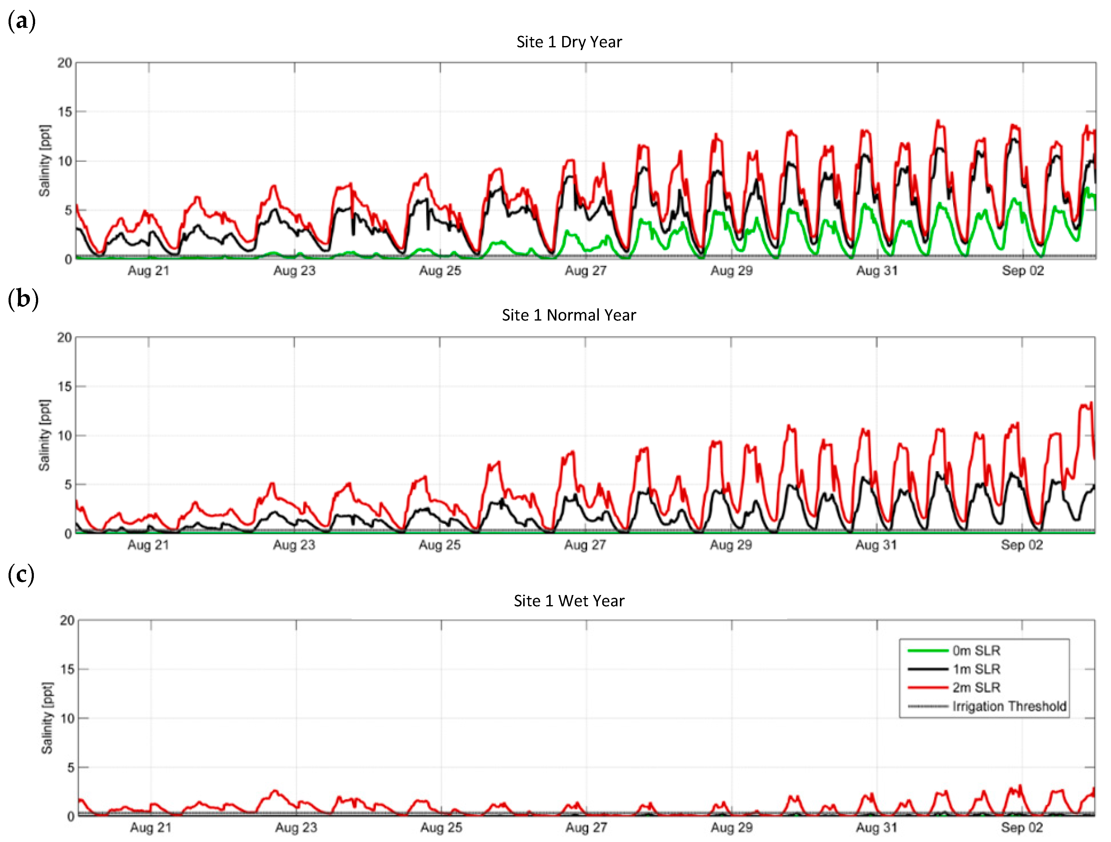
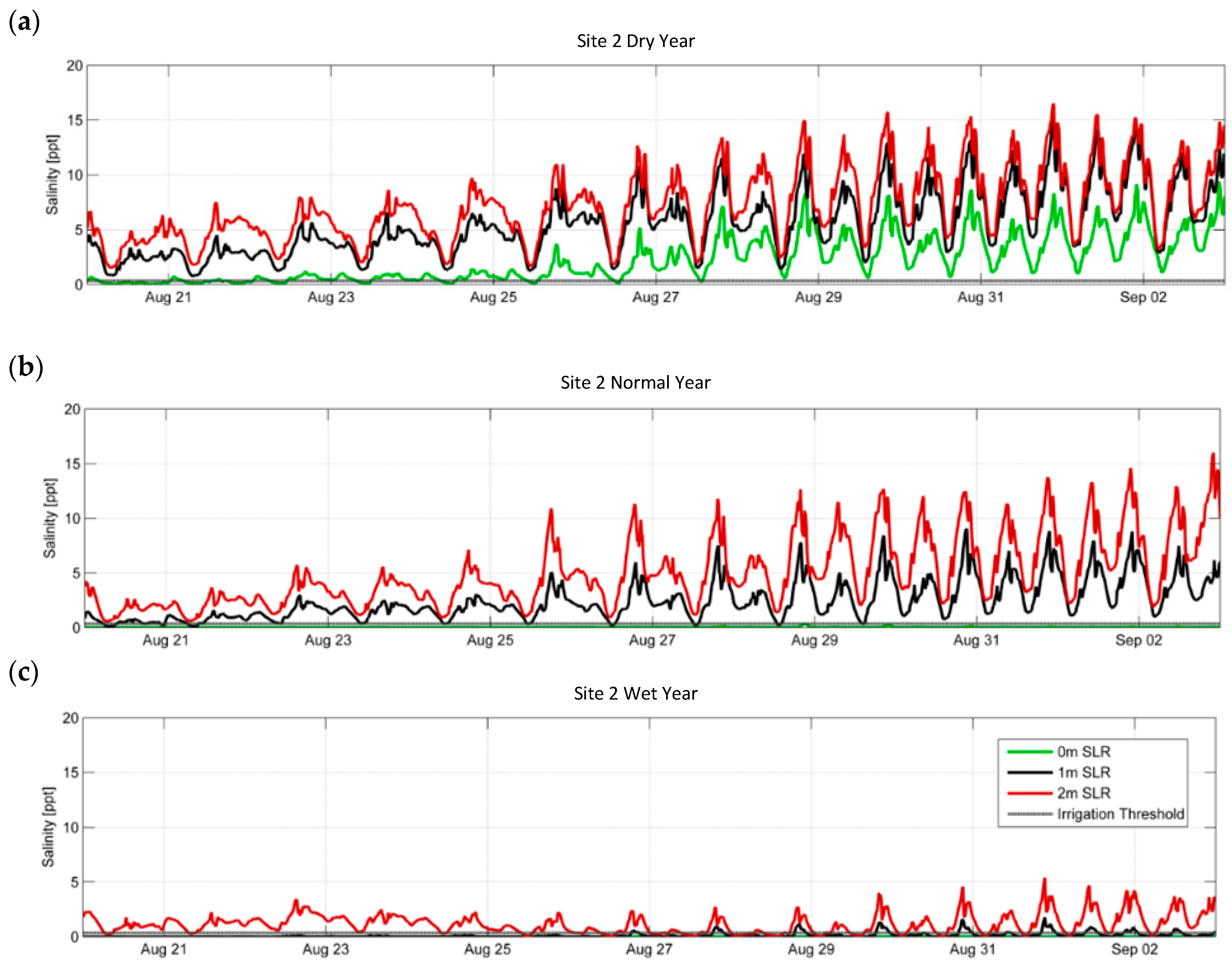
  • Site 1, located 4 km upstream of Site 2, has consistently shown to have a significantly wider window for water availability in all cases and for all criteria compared to Site 2, the present intake location. This indicates that salinity generally decreases in the upstream direction. However, complex hydrodynamic processes would lead to exceptions to the trend.
  • The temporal projection of the withdrawal window is that, even in a wet flow year, the sea level rise of 1 m and 2 m will lead to a large reduction (minimum 85% reduction) in and, in some scenarios, complete elimination of water availability.
  • This study found that sea level rise and changes in river discharge appear to have a larger impact on the withdrawal availability than does channel deepening. In a low river discharge regime, the impact from sea level change is more significant than it is in the high river discharge regime. On the other hand, the influence of changes in river discharge on withdrawal availability decreases when the sea level is higher than it does when the sea level is lower. It is difficult, however, to draw definitive conclusions regarding which factor (sea level rise or river flow) dominates the salt wedge dynamics from this set of model results because, as presented in Section 3.4.1 and in Figure 10, each of the sea level rise cases incorporates different flow rates associated with the projected normal year, dry year, and wet year as predicted by MIROC for its own time horizon (present, year 2050 and year 2100); simply speaking, these model runs have two varying factors, the flow rate and sea level, and it is not immediately obvious which factor is more important in governing the salinity in the river. However, it is difficult to consider one factor without another, considering that the sea level rise and change in the Fraser River hydrograph are both results of climate change.
  • Dredging the channel to accommodate vessels with a 20 m draft will affect the salinity at the intake and will shorten the withdrawal window. The effect of channel deepening becomes more pronounced in the low flow period. However, the degree of impact from dredging on the salt wedge and on withdrawal availability under other different circumstances (i.e., different sea level rise and different dredge depths) have not been investigated.

Author Contributions

Conceptualization, A.T.Y.L., J.S. and J.M.; Methodology, A.T.Y.L. and J.S.; Software, J.S.; Validation, A.T.Y.L. and J.S.; Formal Analysis, A.L and J.M.; Investigation, A.T.Y.L. and J.M.; Resources, J.S.; Visualization, A.T.Y.L. and J.M.; Writing-Original Draft Preparation, A.T.Y.L. and J.S.; Writing-Review & Editing, A.T.Y.L. and J.S.; Supervision, J.S.; A.T.Y.L. and J.M. contributed to the scenarios selection and ensemble analysis; A.T.Y.L., J.S. and J.M. contributed to the modelling, and A.T.Y.L. and J.S. conceived and wrote the paper.

Funding

This study was funded in part by the Corporation of Delta and in part by the Governments of Canada and British Columbia through the Investment Agriculture Foundation of BC under Growing Forward 2, a federal-provincial-territorial initiative. The program was delivered by the BC Agriculture & Food Climate Action Initiative.

Acknowledgments

In addition to the agencies who contributed financially to this project as stated above, the authors would like to acknowledge Delta Farmers Institute, Corporation of Delta and BC Ministry of Agriculture for their role in the project.

Conflicts of Interest

The authors declare no conflict of interest.

Appendix A. Theoretical Basis of H3D

H3D bears many similarities to the Princeton Ocean Model (POM) [42] in terms of the equations it solves, but differs in how the time-domain aspects are implemented. H3D uses a semi-implicit scheme, allowing relatively large time steps, and does not separately solve the internal and external models as POM does. It also uses a considerably simpler turbulence scheme in the vertical. These considerations combined allow H3D to execute complex problems relatively quickly.
The Equations (A1)–(A11) to be solved are detailed below. The explanation of the symbols that are used in these equations is either provided in the text in this appendix or in Appendix B:
Mass Conservation:
u x + v y + w z = 0 ,
At the end of each time step equation, (1) is used to diagnostically determine the vertical component of velocity (w) once the two horizontal components of velocity (u and v) have been calculated by the model.
X-directed momentum:
u t + u u x + v u y + w u z + g η x + 1 ρ o x z η ( ρ w ρ o ) g d z f v x A H u x y A H u y z A V u z = 0
Y-directed momentum:
v t + u v x + v v y + w v z + g η y + 1 ρ o y z η ( ρ w ρ o ) g d z + f u x A H v x y A H v y z A V v z = 0
Water surface elevation determined from the vertically-integrated continuity equation:
η t = x H η u d z y H η v d z  
The effect of wind forcing introduced by means of the surface wind-stress boundary condition:
( A V u z , A V v z ) z = η = ρ a ρ w C D , a i r U w i n d | U w i n d |  
The effect of bottom friction introduced by the bottom boundary condition:
( A V u z , A V v z ) z = H = K b o t t o m U b o t t o m | U b o t t o m |  
The bottom friction coefficient is usually understood to apply to currents at an elevation of one metre above the bottom. The bottom-most vector in H3D will, in general, be at a different elevation, i.e., at the midpoint of the lowest computational cell. H3D uses the ‘law of the wall’ to estimate the flow velocity at one metre above the bottom from the modelled near-bottom velocity.
The evolution of scalars, such as salinity, temperature, or suspended sediment, is given by the scalar transport/diffusion equation:
S t + u S x + v S y + w S z x N H S x y N H S y z N V S z = Q  
The above Equations (A1)–(A7) are formally integrated over the small volumes defined by the computational grid, and a set of algebraic equations results, for which an appropriate time-stepping methodology must be found. Backhaus [18,19] presents such a procedure, referred to as a semi-implicit method. The spatially-discretized version of the continuity equation is written as:
η ( 1 ) = η ( 0 ) α Δ t Δ l ( δ x U ( 1 ) + δ y V ( 1 ) ) ( 1 α ) Δ t Δ l ( δ x U ( 0 ) + δ y V ( 0 ) ) ,
where superscript (0) and (1) refer to the present and the advanced time, δx and δy are spatial differencing operators, and U and V are vertically integrated velocities. The factor α represents an implicit weighting, which must be greater than 0.5 for numerical stability. U(0) and V(0) are known at the start of each computational cycle. U(1), and similarly V(1), can be expressed as:
U ( 1 ) = U ( 0 ) g α Δ t η x ( 1 ) g ( 1 α ) Δ t η x ( 0 ) + Δ t X ( 0 ) ,
where X(0) symbolically represents all other terms in the equation of motion for the u- or v-component, which are evaluated at time level (0): Coriolis force, internal pressure gradients, non-linear terms, and top and bottom stresses. When these expressions are substituted into the continuity Equation (A4), after some further manipulations, there results an elliptic equation for δ i , k , the change in water level over one time step at grid cell i,k (respectively the y and x directions):
δ i , k ( c e δ i , k + 1 + c w δ i , k 1 + c n δ i 1 , k + c s δ i + 1 , k ) = Z i , k ,
where ce, cw, cn, and cs are coefficients depending on local depths and the weighting factor (α), and Zi,k represents the sum of the divergence formed from velocities at time level (0) plus a weighted sum of adjacent water levels at time level (0). Once Equation (A10) is solved for δ i , k , the water level can be updated:
η i , k ( 1 ) = η i , k ( 0 ) + δ i , k ,
and Equation (A9) can be completed. At the end of each time step, volume conservation is used to diagnostically compute the vertical velocity w(j,i,k) from the two horizontal components u and v.

Appendix B. Notations

This appendix explains the symbols used in Equations (A1)–(A11) that were not explained explicitly in Appendix A.
u(x,y,z,t): component of velocity in the x direction
v(x,y,z,t): component of velocity in the y direction
w(x,y,z,t): component of velocity in the z direction
S(x,y,z,t): scalar concentration
Q(x,y,z,t): source term for each scalar species
f: Coriolis parameter, determined by the earth’s rotation and the local latitude
AH ( u / x , u / y , v / x , v / y ) : horizontal eddy viscosity
AV ( u / z , v / z , ρ w a t e r / z ) : vertical eddy viscosity
NH: horizontal eddy diffusivity
NV ( u / z , v / z , ρ w a t e r / z ) : vertical eddy diffusivity
CD,air: drag coefficient at the air-water interface
Kbottom: drag coefficient at the water/sea bottom interface
ρa: density of air
ρw(x,y,z,t): density of water
ρo: reference density of water
η(x,y,t): water surface elevation
H(x,y): local depth of water.

References

  1. Costanza, R.; D’Arge, R.; De Groot, R.; Farber, S.; Grasso, M.; Hannon, B.; Limburg, K.; Naeem, S.; O’Neill, R.V.; Paruelo, J.; et al. The value of the world’s ecosystem services and natural capital. Nature 1997, 387, 253–260. [Google Scholar] [CrossRef]
  2. Stronach, J.A. Observational and Modelling Studies of the Fraser River Plume. Ph.D. Thesis, The University of British Columbia, Vancouver, BC, Canada, 1978. [Google Scholar]
  3. Stronach, J.A. The Fraser River plume, Strait of Georgia. Ocean Manag. 1981, 6, 201–221. [Google Scholar] [CrossRef]
  4. Halverson, M.; Pawlowicz, R. Tide, wind, and river forcing of the surface currents in the Fraser River plume. Atmos. Ocean 2016, 54, 131–152. [Google Scholar] [CrossRef]
  5. Halverson, M.; Pawlowicz, R. Entrainment and flushing time in the Fraser River estuary and plume from a steady state salt balance analysis. J. Geophys. Res.-Atmos. 2011, 116. [Google Scholar] [CrossRef]
  6. Halverson, M.; Pawlowicz, R. Estuarine forcing of a river plume by river flow and tides. J. Geophys. Res.-Atmos. 2008, 113. [Google Scholar] [CrossRef] [Green Version]
  7. Kostaschuk, R.; Atwood, L.A. River discharge and tidal controls on salt-wedge position and implications for channel shoaling: Fraser River, British Columbia. Can. J. Civ. Eng. 2011, 17, 452–459. [Google Scholar] [CrossRef]
  8. Ward, P.R.B. Seasonal salinity changes in the Fraser River estuary. Can. J. Civ. Eng. 2011, 3, 342–348. [Google Scholar] [CrossRef]
  9. Yin, K.D.; Harrison, P.J.; Pond, S.; Beamish, R.J. Entrainment of nitrate in the Fraser River estuary and its biological implications. III. Effects of winds. Estuar. Coast. Shelf Sci. 1995, 40, 545–558. [Google Scholar] [CrossRef]
  10. Neilson-Welch, L.; Smith, L. Saline water intrusion adjacent to the Fraser River, Richmond, British Columbia. Can. Geotech. J. 2011, 38, 67–82. [Google Scholar] [CrossRef]
  11. Krvavica, N.; Travaš, V.; Ožanić, N. Salt-Wedge Response to Variable River Flow and Sea-Level Rise in the Microtidal Rječina River Estuary, Croatia. J. Coast. Res. 2017, 33, 802–814. [Google Scholar] [CrossRef]
  12. Funahashi, T.; Kasai, A.; Ueno, M.; Yamashita, Y. Effects of short time variation in the river discharge on the salt wedge intrusion in the Yura Estuary, Japan. J. Water Resour. Prot. 2013, 5, 343–348. [Google Scholar] [CrossRef]
  13. Shaha, D.C.; Cho, Y.K.; Kim, T.W. Effects of river discharge and tide driven variation on saltwater intrusion in Sumjin River Estuary: An application of finite-volume coastal ocean model. J. Coast. Res. 2013, 29, 460–470. [Google Scholar] [CrossRef]
  14. Richmond Chamber of Commerce. The Economic Importance of the Lower Fraser River; Richmond Chamber of Commerce: Richmond, BC, Canada, 2014. [Google Scholar]
  15. Crawford, E.; MacNair, E. Fraser Valley & Metro Vancouver Snapshot Report, B.C. Agriculture Climate Change Adaptation Risk + Opportunity Assessment Series; The British Columbia Agriculture & Food Climate Action Initiative: Victoria, BC, Canada, 2012. [Google Scholar]
  16. Van der Gulik, T.; Neilsen, D.; Fretwell, R.; Tam, S. Agricultural Water Demand Model—Report for Metro Vancouver; Metro Vancouver: Vancouver, BC, Canada, 2014. [Google Scholar]
  17. Backhaus, J.O. A semi-implicit scheme for the shallow water equations for applications to shelf sea modelling. Cont. Shelf Res. 1983, 2, 243–254. [Google Scholar] [CrossRef]
  18. Backhaus, J.O. A three-dimensional model for the simulation of shelf-sea dynamics. Deutsche Hydro. Z. 1985, 38, 165–187. [Google Scholar] [CrossRef]
  19. Duwe, K.C.; Hewer, R.R.; Backhaus, J.O. Results of a semi-implicit two-step method for the simulation of markedly non-linear flow in coastal seas. Cont. Shelf Res. 1983, 2, 255–274. [Google Scholar] [CrossRef]
  20. Backhaus, J.O.; Meir-Reimer, E. On seasonal circulation patterns in the North Sea. In North Sea Dynamics; Sundermann, J., Lenz, W., Eds.; Springer: Heidelberg, Germany, 1983; pp. 63–84. ISBN 978-3-642-68840-9. [Google Scholar]
  21. Kampf, J.; Backhaus, J.O. Ice-ocean interactions during shallow convection under conditions of steady winds: Three-dimensional numerical studies. Deep-Sea Res. Part II 1999, 46, 1335–1355. [Google Scholar] [CrossRef]
  22. Backhaus, J.O.; Kampf, J. Simulation of sub-mesoscale oceanic convection and ice-ocean interactions in the Greenland Sea. Deep-Sea Res. Part II 1999, 46, 1427–1455. [Google Scholar] [CrossRef]
  23. Stronach, J.A.; Backhaus, J.O.; Murty, T.S. An update on the numerical simulation of oceanographic processes in the waters between Vancouver Island and the mainland: The G8 model. Oceanogr. Mar. Biol. 1999, 31, 1–86. [Google Scholar]
  24. Stronach, J.A.; Mulligan, R.P.; Soderholm, H.; Draho, R.; Degen, D. Okanagan lake limnology: Helping to improve water quality and safety. In Innovation; Association of Professional Engineers and Geoscientists of British Columbia: Vancouver, BC, Canada, 2002. [Google Scholar]
  25. Wang, E.; Stronach, J.A. Summerland water intake feasibility study. In Proceedings of the Canadian Water Resources Association BC Branch Conference, Kelowna, BC, Canada, 23–25 February 2005. [Google Scholar]
  26. Saucier, F.J.; Roy, F.; Gilbert, D.; Pellerin, P.; Ritchie, H. The formation of water masses and sea ice in the Gulf of St. Lawrence. J. Geophys. Res. 2003, 108, 3269–3289. [Google Scholar] [CrossRef]
  27. Rego, J.L.; Meselhe, E.; Stronach, J.A.; Habib, E. Numerical modelling of the Mississippi-Atchafalaya rivers’ sediment transport and fate: Considerations for diversion scenarios. J. Coast. Res. 2010, 26, 212–229. [Google Scholar] [CrossRef]
  28. Arakawa, A.; Lamb, V.R. Computational design of the basic dynamical processes of the UCLA general circulation model. Methods Comput. Phys. 1977, 17, 173–263. [Google Scholar]
  29. Smagorinsky, J. General circulation experiment with the primitive equations: I. the basic experiment. Mon. Weather Rev. 1963, 91, 99–164. [Google Scholar] [CrossRef]
  30. Mellor, G.L.; Yamada, T. Development of a turbulent closure model for geophysical fluid problems. Rev. Geophys. 1982, 20, 851–875. [Google Scholar] [CrossRef]
  31. Mellor, G.L.; Durbin, P.A. The structure and dynamics of the ocean surface mixed layer. J. Phys. Oceanogr. 1975, 5, 718–728. [Google Scholar] [CrossRef]
  32. Zalesak, S.T. Fully multidimensional flux-corrected transport algorithms for fluids. J. Comput. Phys. 1979, 31, 335–362. [Google Scholar] [CrossRef]
  33. Kondratyev, K.Y. Radiation Processes in the Atmosphere; No. 309; World Meteorological Organization, The University of California: San Diego, CA, USA, 1972. [Google Scholar]
  34. Gill, A.E. Atmosphere-Ocean Dynamics; Academic Press: London, UK, 1982. [Google Scholar]
  35. Crean, P.B.; Ages, A.B. Oceanographic Records from Twelve Cruises in the Strait of Georgia and Juan de Fuca Strait, 1968; Department of Energy, Mines and Recources, Marine Research Sciences Branch: Ottawa, ON, Canada, 1971. [Google Scholar]
  36. Water Survey of Canada. Available online: https://www.canada.ca/en/environment-climate-change/services/water-overview/quantity/monitoring/survey.html (accessed on 15 February 2016).
  37. The Intergovernmental Panel on Climate Change. Climate Change 2007: The Fourth Assessment Report; Cambridge University Press: New York, NY, USA, 2007. [Google Scholar]
  38. Werner, A.T. BCSD Downscaled Transient Climate Projections for Eight Select GCMs over British Columbia, Canada; Pacific Climate Impacts Consortium, University of Victoria: Victoria, BC, Canada, 2011. [Google Scholar]
  39. Schnorbus, M.A.; Bennett, K.E.; Werner, A.T.; Berland, A.J. Hydrologic Impacts of Climate Change in the Peace, Campbell and Columbia Watersheds, British Columbia, Canada; Pacific Climate Impacts Consortium, University of Victoria: Victoria, BC, Canada, 2011. [Google Scholar]
  40. Pacific Climate Impact Consortium. Available online: https://www.pacificclimate.org (accessed on 1 February 2016).
  41. Ausenco Sandwell. Sea Dike Guidelines; BC Ministry of Environment: Victoria, BC, Canada, 2011; pp. 4–5. [Google Scholar]
  42. Blumberg, A.F.; Mellor, G.L. A description of a three-dimensional coastal circulation model. In Three-Dimensional Coastal Ocean Models; Heaps, N.S., Ed.; American Geophysical Union: Washington, DC, USA, 1987; pp. 1–16. [Google Scholar]
Figure 1. Study location of the Fraser River estuary.
Jmse 06 00130 g001
Figure 2. Typical grid mesh used in H3D.
Jmse 06 00130 g002
Figure 3. Nesting of the 1-km Strait of Georgia (SOG) model, the 50-m Fraser River model, and the one-dimensional Fraser River model.
Jmse 06 00130 g003
Figure 4. Fraser River flow rate at Hope in 2011.
Jmse 06 00130 g004
Figure 5. Comparison of observed and modelled results: (a) water level and (b) conductivity in the Fraser River.
Jmse 06 00130 g005aJmse 06 00130 g005b
Figure 6. Modelled salinity at 2-m depth in the Fraser River on 11 November 2011 at 7 a.m.
Jmse 06 00130 g006
Figure 7. Comparison of observed and modelled available water withdrawal hours in November.
Jmse 06 00130 g007
Figure 8. Ensemble historical and modelled daily Fraser River flow rate.
Jmse 06 00130 g008
Figure 9. Comparison of observed and modelled Fraser River flow rate for years 1998–2004.
Jmse 06 00130 g009
Figure 10. Statistical comparison of selected hydrographs for various timeframes: (a) present timeframe; (b) year 2050 timeframe; (c) year 2100 timeframe.
Jmse 06 00130 g010aJmse 06 00130 g010b
Figure 11. Location of candidate sites for additional water intake installation.
Jmse 06 00130 g011
Figure 12. Modelled surface salinity at site 1, site 2, and site 3 in September: (a) 8–11 September; (b) 22–25 September.
Jmse 06 00130 g012aJmse 06 00130 g012b
Figure 13. Surface salinity at site 2 between August and October in normal flow year and with 0-m SLR: (a) August; (b) September; (c) October.
Jmse 06 00130 g013aJmse 06 00130 g013b
Figure 14. Surface salinity at site 1 in August with 0–2 m SLR: (a) dry year; (b) normal year; (c) wet year.
Jmse 06 00130 g014
Figure 15. Surface salinity at site 2 in August with 0–2 m SLR: (a) dry year; (b) normal year; (c) wet year.
Jmse 06 00130 g015
Figure 16. Surface salinity at site 3 in August with 0–2 m SLR. (a) dry year; (b) normal year; (c) wet year.
Jmse 06 00130 g016
Figure 17. Time series salinity at site 2 with river channel depth capable of accommodating vessels drafting 11.5 m and 20.0 m with 0-m SLR during irrigation period. (a) August; (b) September; (c) October.
Jmse 06 00130 g017
Table 1. Modelling sequence of the study.
Seq. #ModelInitial ConditionsDownstream Boundary ConditionsUpstream Boundary ConditionsDynamic Model CouplingObjective
1a1-km SOG Temperature and salinity profilesTemperature, salinity and tidal levelFlow conditions provided by the 1-D Fraser River model1-D Fraser River model for the 1-km SOG modelTo provide boundary conditions to the 50-m Fraser River Model
1b1-D Fraser River-for the 1-km SOGWater levelWater level from the 1-km SOG modelRiver hydrograph at Hope1-km SOG modelTo provide upstream boundary conditions to the 1-km SOG model
2a50-m Fraser RiverTemperature and salinity profiles Temperature, salinity and tidal level provided by the SOG modelFlow conditions provided by the 1-D Fraser River model 1-D Fraser River model for the 50-m Fraser River modelTo simulate spatial and temporal salinity distributions in the Fraser River
2b1-D Fraser River-for the 50-m Fraser RiverWater levelWater level from the 1-km SOG modelRiver hydrograph at Hope50-m Fraser River modelTo provide upstream boundary conditions to the 50-m Fraser River model
Table 2. Climate scenarios and the associated social, economic, and human theme as presented in AR4.
Climate ScenarioDescriptionCharacteristics
A1BThis scenario is of a more integrated world
  • Rapid economic growth
  • A global population that reaches 9 billion in 2050 and then quickly declines
  • The quick spread of new and efficient technologies
  • A convergent world—income and way of life converge between regions. Extensive social and cultural interactions worldwide
  • Good balance on all different types of energy sources
A2These scenarios are of a more divided world
  • A world of independently operating, self-reliant nations
  • Continuously increasing population
  • Regionally oriented economic development
B1This scenario is of a world more integrated, and more ecologically friendly
  • Rapid economic growth as in A1, but with rapid changes towards a service and information economy
  • Population rising to 9 billion in 2050 and then declining as in A1
  • Reductions in material intensity and the introduction of clean and resource efficient technologies.
  • An emphasis on global solutions to economic, social, and environmental stability
Table 3. Fraser River hydrograph chosen for the ensemble analysis.
TimeframeYear of Chosen Hydrographs for Ensemble AnalysisType of Data
Present (2014) 2005–2014Observed
20502045–2055Predicted based on MIROC
21002089–2098 1Predicted based on MIROC
1 2098 is the end of the river flow prediction based on MIROC published by PCIC as at the time of the study.
Table 4. Modelled time duration (no. of hours) below salinity criterion of 0.34 ppt at site 1, site 2, and site 3 with various sea level rises and types of flow year.
Site 1 (h)Site 2 (h)Site 3 (h)
Sea Level RiseDryNormalWetDryNormalWetDryNormalWet
0 m 7.924.024.03.623.924.03.123.024.0
1 m0.03.823.60.00.821.20.00.418.1
2 m0.00.18.30.00.03.90.00.01.7
Table 5. Time duration below salinity criterion of 0.34 ppt at site 1 and site 2 with 0-m SLR with river channel accommodating vessels with 11.5-m and 20.0-m drafts.
Site 1Site 2
Month11.5-m Draft
(h/Day)
20.0-m Draft
(h/Day)
11.5-m Draft
(h/Day)
20.0-m Draft
(h/Day)
August24.019.823.915.0
September22.06.116.91.1
October15.02.39.90.5

