Asymmetric Deep Co-Training Framework Using a Shape Context Descriptor for Reservoir Prediction: A Case Study from the Yinggehai Basin, South China Sea

Abstract

The scarcity and incompleteness of well-log data pose a critical challenge to deep learning-based reservoir prediction. To address this small-sample problem and improve prediction quality, we propose a novel semi-supervised asymmetric deep co-training framework integrated with a shape context descriptor. This method leverages abundant unlabeled seismic data as well as complementary information on related physical properties. Specifically, we introduce a shape context descriptor to encode seismic waveform morphology and spatial context, thereby improving the lateral continuity and interpretability of predictions while mitigating issues inherent in the sequence-to-point paradigm, wherein three-dimensional seismic data are used as input and a single target point is predicted. To overcome data limitations, a sliding-window resampling strategy is employed to expand the training samples. For co-training, we design an asymmetric dual-task architecture wherein one model performs porosity regression while the other conducts reservoir type classification, thereby enabling synergistic learning. The proposed framework is validated using real three-dimensional seismic data from the Yinggehai Basin in the South China Sea through ablation experiments. The results demonstrate superior performance in prediction accuracy, spatial consistency, and training stability compared to baseline methods.

1. Introduction

Oil and gas production typically peaks during the early stages of field development. With time, the need for development plans grounded in rigorous theoretical foundations and robust empirical evidence increases. As exploration targets shift toward deeper and more complex reservoirs, characterization and evaluation of these reservoirs become increasingly challenging.

Physical properties are essential for evaluating oil and gas reservoirs. Typically, pre-stack or post-stack seismic inversion methods are used to estimate elastic parameters; subsequently, reservoir physical properties, such as porosity and permeability, are predicted based on established statistical relationships [1,2]. Porosity indicates a reservoir’s capacity to store fluids by measuring the proportion of rock volume occupied by pore space available for fluids such as oil, gas, or water. It is a key indicator for assessing whether a reservoir can store sufficient hydrocarbons. Permeability reflects how easily fluids flow through a rock’s pore network by quantifying the ease of flow through interconnected pores within reservoir rocks. It is one of the most important parameters for evaluating a reservoir’s commercial viability, production prospects, and recoverability. Therefore, porosity and permeability are considered among the most significant physical properties of reservoir rocks [3]. These parameters are fundamental to the assessment of reservoir quality and the development of effective extraction strategies [4]. Currently, the primary methods for obtaining porosity and permeability data include laboratory core testing and indirect inversion techniques [5]. Laboratory testing provides the most accurate data; however, due to cost constraints, cores are typically extracted only from a limited number of key wells during exploration. Indirect inversion estimates these properties by exploiting relationships between porosity and permeability and seismic data or elastic parameters [6]. However, the relationship between physical properties and seismic data is highly nonlinear. The accuracy of property predictions is affected by uncertainties in seismic inversion and ambiguities in rock-physical relationships. These uncertainties can propagate throughout the workflow, thereby increasing prediction errors [7].

Deep learning is a class of neural network models used to approximate aspects of human brain function for analysis and learning tasks. The key advantage of deep learning lies in its ability to solve specific problems by constructing task-appropriate network architectures. By introducing unprecedented efficiency and innovation, it has a profound impact on traditional upstream geothermal energy industries, such as geothermal energy, oil, and natural gas industries [8]. It has applications in seismic data processing, such as seismic data denoising and data reconstruction [9,10]. Deep learning is also used in seismic reservoir prediction, including lithology and fluid content prediction [11,12], fracture property prediction [13,14,15], fault interpretation [16], and reservoir parameters prediction (e.g., porosity, permeability) [17,18,19].

Existing methods for constructing sample pairs based on logging data can broadly be categorized into three types: PTP (point to point), STP (sequence to point), and STS (sequence to sequence) [20]. PTP does not account for the spatial linkage between the logging sampling points and the surrounding strata. STP can make it difficult for the network to capture features when reservoir parameter changes [21], whereas establishing the STS prediction paradigm places high demands on logging data and requires numerous continuous logging labels. Due to the environmental conditions and cost limitations, logging data often contains several missing values. Moreover, during deep learning sample construction, it is necessary to transform data from the depth domain to the time domain, which involves downsampling. Although mask-based loss functions can alleviate the problem of sparse labeling, missing values may still affect model performance [20].

The small-sample problem has also attracted considerable research attention within the field of deep learning research. To address well-log scarcity, semi-supervised learning (SSL) in geophysics has evolved from traditional machine learning (e.g., using TSVM for anomaly detection [22]) to modern deep consistency regularization. While frameworks like Mean Teacher succeed in discrete classification tasks such as salt segmentation [23], applying these homogeneous methods to continuous petrophysical regression under ultra-sparse labels often leads to optimization bottlenecks and numerical confusion [24]. In computer vision sample expansion, early approaches employed data augmentation methods based on fundamental image transformations to address the scarcity of image samples. These methods are simple and efficient and remain among the most used techniques. They achieve augmentation through geometric transformations (e.g., rotation, translation, cropping, scaling, etc.) or color transformations in pixel space [25]. However, seismic data differ substantially from traditional natural images. Adjacent channels in seismic data contain crucial geological information, and inappropriate alterations may compromise their physical significance. Therefore, simple rotation or stitching techniques cannot be directly applied to augment seismic datasets. With advances in generative networks, deep learning–based sample generation has seen increasing applications, exemplified by generative adversarial networks (GANs) and diffusion models. These methods learn data distributions to generate more complex and realistic images. Generative model–based sample augmentation has also been applied in seismic denoising [26,27] and reservoir facies generation [28]. However, these models are difficult to train and generate samples that exhibit artifacts and blurring. While these issues can be manually controlled for relatively large image datasets, generated errors become difficult to control in smaller-scale reservoir parameter prediction because the quality of generated samples cannot be empirically measured.

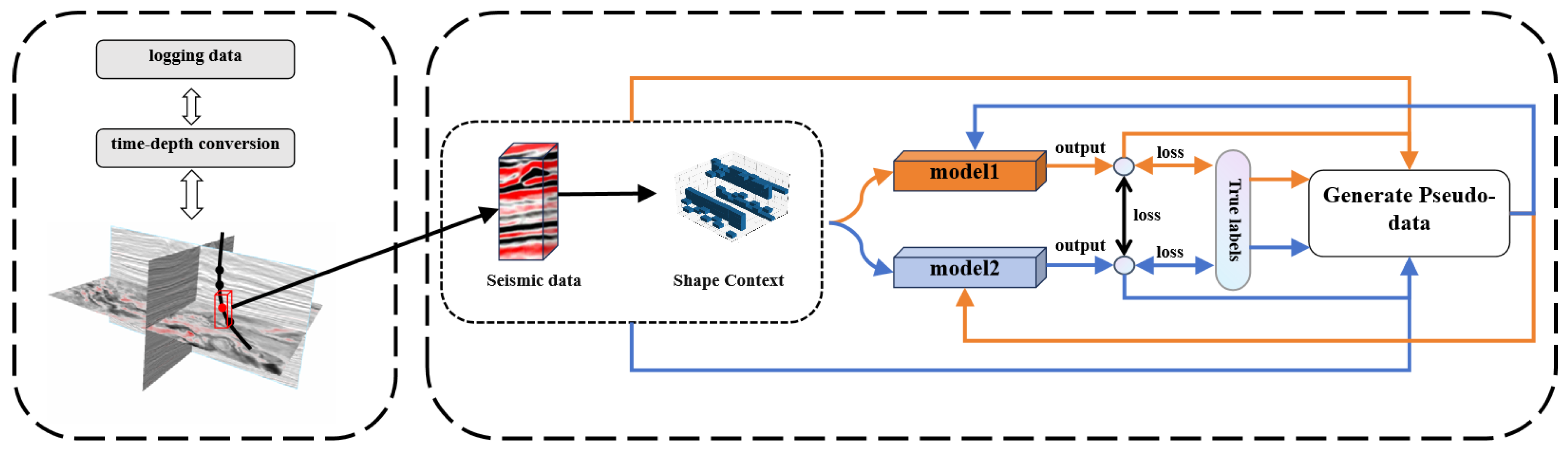
This paper combines a semi-supervised learning framework that utilizes deep co-training and shape context and employs different models for two distinct tasks. Specifically, shape context explicitly encodes seismic waveform information and the relative spatial positions of prediction points, thereby addressing the issue where the model cannot accurately capture features at label transitions. The deep co-training framework introduces a large amount of unlabeled data and adversarial sample generation methods, thereby alleviating the problem of sample sparsity. Figure 1 depicts the workflow of this paper, which includes sample construction, the model training process, and network architecture. First, we apply shape context to seismic data and the dataset construction process, including the sample expansion strategy. Subsequently, we describe the details of applying deep co-training to reservoir prediction. Finally, we demonstrate the effectiveness of the proposed method by applying it to real seismic data.

Compared with existing reservoir prediction methods, the primary contributions and novelties of this work are highlighted in the following two aspects:

(1)

In complex geological environments such as the tight sandstone reservoirs in the South China Sea, the porosity data derived from well logs typically exhibits a relatively continuous distribution. In contrast, the corresponding permeability data is heavily influenced by microscopic pore-throat structures, demonstrating extreme heterogeneity. Compounded by the overall scarcity of well-log data, accurate quantitative prediction of permeability is highly challenging. Therefore, this study adopts a combined approach utilizing porosity regression and permeability classification. Furthermore, the effectiveness of deep co-training relies on the assumption of divergent input perspectives between the two models. Our proposed asymmetric training framework, which integrates different task types (quantitative and qualitative), further amplifies this perspective variance, compelling the models to perform deeper cross-validation of physical information.

(2)

Traditional Sequence-to-Point (STP) deep learning prediction paradigms typically treat individual seismic traces as isolated sequences. Due to their reliance on fixed sliding windows, these models struggle to capture features when reservoir parameters change abruptly. Conventional STP models depend heavily on absolute seismic amplitudes or standard attributes and lack sensitivity to the topological shape of the waveform (i.e., the relative geometric morphology of peaks and troughs). Consequently, they are prone to producing laterally discontinuous “vertical stripes” in profile predictions. By introducing the Shape Context descriptor to explicitly encode the relative spatial position and two-dimensional geometric distribution of target points within the seismic waveform, we achieve a feature-based representation of waveform morphology. This approach not only compensates for the deficiencies in conventional sequential feature extraction but also significantly enhances the lateral continuity and geological interpretability of the spatial prediction results.

2. Methodology

2.1. Shape Context

Compared with other waveform feature representations, Shape Context (SC) descriptors offer unique advantages and are particularly well-suited for STP prediction paradigms. However, the STP paradigm struggles to capture corresponding feature changes at label boundaries, especially at lithological interfaces, making it difficult for the network to learn feature transitions across reservoir boundaries. Moreover, most alternative waveform descriptors focus on local signal features or spectral characteristics, often losing the clear spatial and geometric shape of the waveform. In contrast, shape context descriptors explicitly encode the relative spatial positions between waveform morphology and the predicted points. We therefore believe that shape descriptors are more appropriate for the task requirements of this study. Shape context descriptors have also been applied in the field of geophysics [29,30]. As core data in seismic exploration, waveform data contains crucial information reflecting subsurface structures, reservoir characteristics, and the distribution of hydrocarbons. By deeply mining the rich reservoir information embedded in seismic waveforms, it is possible to optimize reservoir prediction results, enhance the accuracy of reservoir characterization, and thereby improve drilling efficiency. In specific applications, seismic waveforms record important characteristics related to stratigraphic lithology and structural features. By comparing the similarity of waveform shapes, spatial distribution patterns of strata can be systematically revealed [31]. Shape context is a shape descriptor designed to solve the non-rigid shape matching problems by statistically characterizing the spatial distribution of points around a contour [32]. Its core concept involves describing a point using its “perspective” within the surrounding environment. By comparing the “perspectives” of all points, the method measures the similarity between two overall shapes. This approach exhibits robustness to noise and invariance to translation, scaling, and minor deformation. With the development of deep learning, there are more and more examples of combining shape context with deep learning [33,34]. Single-channel seismic data, as a time series, exhibit a two-dimensional shape within an STP-based prediction paradigm. A seismic trace is represented by the time series ${S=\{S}_j,\dots ,S_N\}$. Using the sampling point ${ S}_k(1\le K\le N)$ as the origin, a logarithmic polar coordinate system is established to represent a two-dimensional shape. The standard amplitude difference is first calculated for sequences within the window using the following formula:

$$A_{kj}={\displaystyle \frac{abs\left(S_k-S_j\right)-{\mu }_A}{{\sigma }_A}}$$

(1)

where ${\mu }_A$ is the mean value of the amplitude difference within the window, ${\sigma }_{A }$ is the corresponding standard deviation, and $S_j$ denotes another point within the window. The angular information is computed for the reference point and each sampling point within a window, after which it is divided into M intervals. To represent the relative position of the origin more explicitly, we use the index of each point in the sequence rather than computing the Euclidean distance between the origin and each point. The specific calculations are as follows:

$$\{\begin{array}{c}{\theta }_{kj}=arctan2\left(∆A_{kj},j-k\right)mod2\pi \\ r_{kj}=j\end{array}$$

(2)

where $j$ represents the relative position of the target point $S_j$ in the sequence, and $k$ represents the relative coordinate position of the point $S_k$. The number of points falling into each partition relative to the origin is counted to form a histogram. The histogram reflects the spatial distribution characteristics around the origin as well as its relative spatial position within the seismic sequence. The histogram is formed in the following manner:

$$\{\begin{array}{c}{H}_k\left(b_{\theta },b_r\right)={\displaystyle \sum _{j=1}^N}\delta \left({\theta }_{kj}\in b_{\theta },r_{kj}\in b_r\right)\\ \left(b_{\theta },b_r\right)\leftarrow \left({\theta }_{kj},r_{kj}\right)\end{array}$$

(3)

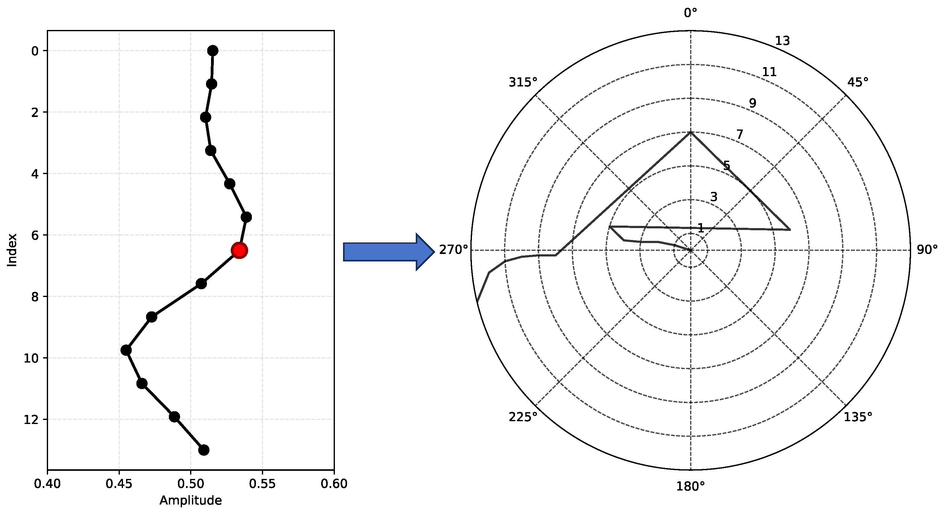
where $\delta (·)$ is an indicator function, taking the value of 1 if the condition is met, and 0 otherwise (If and only if the polar coordinate feature $\left({\theta }_{kj},r_{kj}\right)$ of sampling point j falls within a specific angle bin $b_{\theta }$ and distance bin $b_r$, the value of this function is 1, otherwise it is 0), $(b_{\theta },b_r)\leftarrow \left({\theta }_{kj},r_{kj}\right)$ maps the “angle + distance” feature of point j to the corresponding bin. Specifically, the definition of the angular and distance bins is optimized for 1D seismic sequences. The angular bins ($b_{\theta }$) are generated by uniformly dividing the entire [0, 2$\pi$) angular space into M equal intervals (in this study, M = 13, with each bin spanning $\pi$/6, $b_{\theta 1} = [$0,π/12), $b_{\theta 2}$= [π/12,π/6), with angle 0 assigned to its own separate interval). For the distance bins ($b_r$), unlike the logarithmic distance scaling conventionally used in 2D image processing, we directly utilize the relative time-step index within the sliding window. Because our temporal sampling window length is fixed at N = 13, the distance bins are strictly defined as N discrete integer intervals ($b_r\in \{1,2,\dots ,13\}$). ${ H}_k$ is the shape context histogram, and Figure 2 illustrates the mapping of single-channel seismic data to polar coordinates.

Using the above method, we can obtain a shape context descriptor for a seismic record of length N. This descriptor incorporates the relative spatial positions of the reference points. We compute shape contexts for all seismic traces within a 3D window, concatenate them in the third dimension in the order of inline and crossline, and input them separately from the seismic data into the network, where feature fusion occurs at the fusion layer.

2.2. Extending Labeled Dataset

In deep learning, data are the cornerstone of a model’s capabilities, and their quality fundamentally determines the upper limit of task performance. The learning dataset greatly influences the efficacy of network models and training algorithms in realizing this performance potential. This principle is particularly critical in the context of reservoir prediction tasks in the geophysical domain, which aim to establish complex nonlinear mapping between inputs such as seismic data and reservoir parameter labels. However, the reliability of this mapping relationship is largely limited by dataset quality: sparse and insufficiently diverse samples are the main bottlenecks constraining the model’s generalization ability. To overcome this data bottleneck, it is crucial to effectively expand the training samples to improve the model’s generalization ability. To this end, we propose a shape context–based data expansion method, which aims to generate high-quality and geologically meaningful synthetic samples from limited original samples, thereby providing a more adequate learning foundation for deep learning models.

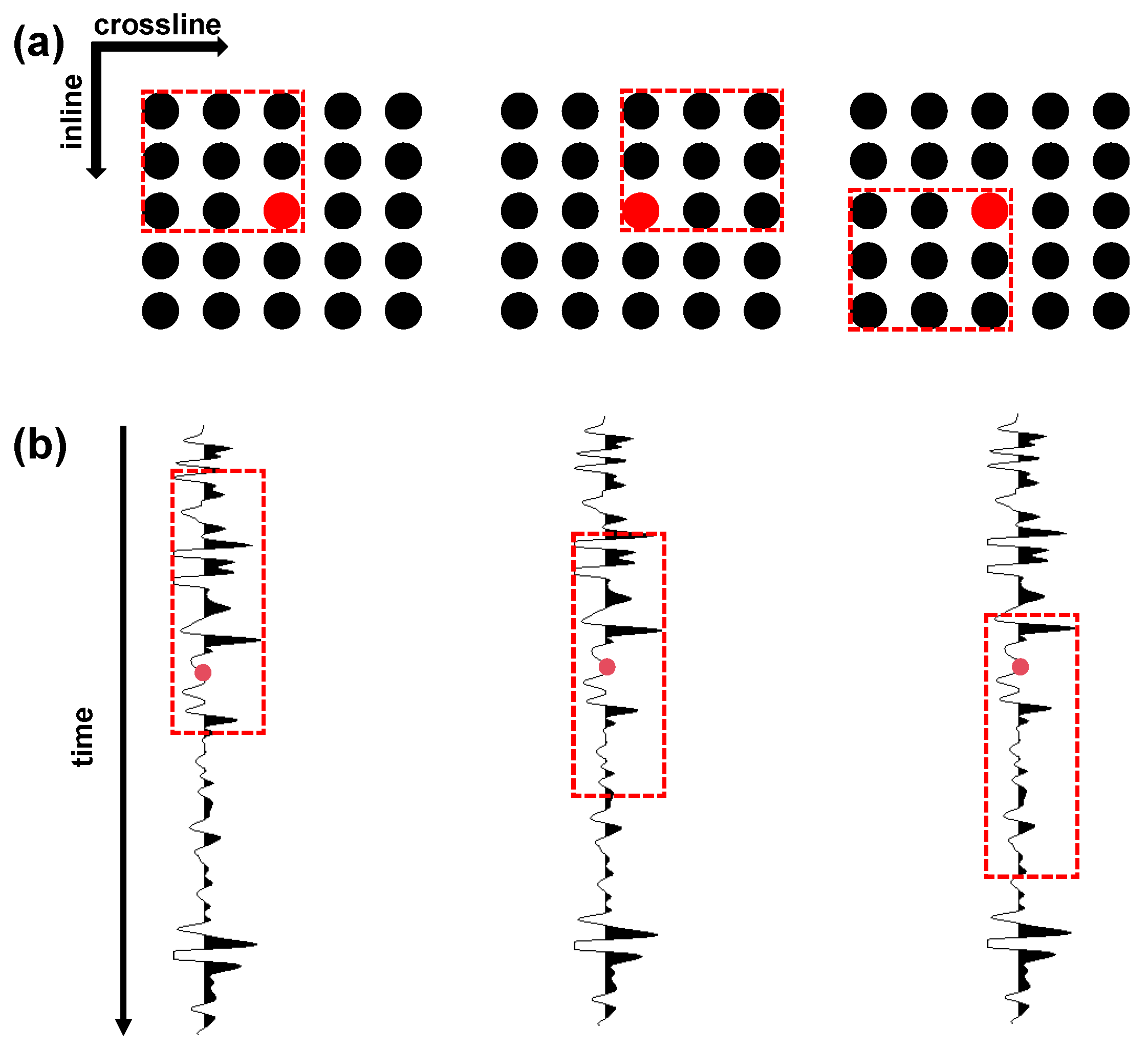
As shown in Figure 3, in the horizontal direction, we consider geological continuity and employ a larger M × M window, within which an N × N sampling window is slid. For example, with a horizontal sampling window size of 3 × 3, we select a larger window of 6 × 6 around the sampling point, thereby obtaining nine samples in the horizontal direction. In the longitudinal direction, resampling is performed in combination with the shape context but changing the relative position of the origin within the window. For example, within a window with a longitudinal length of 13, the sampling point is placed at indices ranging from 1 to 13. In other words, for a sample point on a log, a 3 × 3 × 13 window is used to extract samples, from which 9 × 13 expanded samples can be obtained.

2.3. Dual-Task Deep Co-Training

DCT is a generalized framework based on co-training, the core idea of which is to use two independent views of a dataset to train two models and then exchange information learned from unlabeled datasets [35].

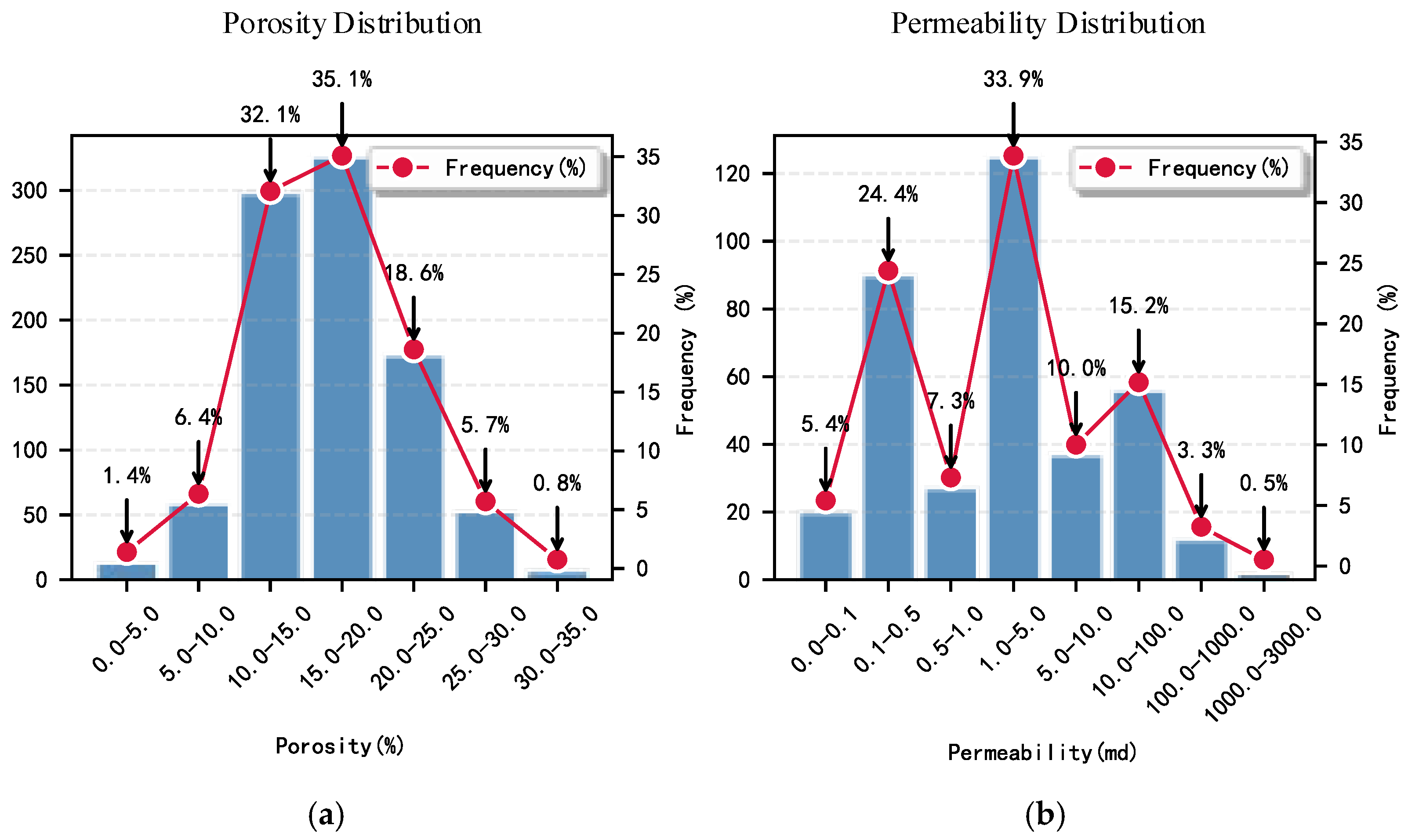
In general, the two trained models are designed to perform a single task. In this study, we aim to predict reservoir porosity and permeability; however, quantitative prediction of permeability is challenging because it is generally more difficult to measure than porosity, and samples are relatively sparse. As shown in Figure 4, the porosity distribution ranges from 0 to 35% and generally follows a normal distribution. Meanwhile, permeability values span from 0 to 3000 md across the samples, exhibiting a more dispersed distribution.

Our goal is to integrate two distinct types of physical measurement data during the model training process. The porosity and permeability values in well logging data may overlap, or one may represent a subset of the other. We intend to leverage the differences between these two measurement types to gain deeper insights during the training of each task. Although one parameter can be predicted from the other using an empirical formula, this approach may introduce errors. Therefore, we designed a dual-task collaborative model for quantitative prediction of porosity and qualitative prediction of permeability. The permeability classification thresholds presented in

Table 1. Classification method for reservoir types.

Permeability (md)	Reservoir Type
>5	1
1~5	2
0.5~1.0	3
0.2~0.5	4
0.1~0.2	5
<0.1	6

are established based on the petroleum and natural gas industry standard of the People’s Republic of China (SY/T 6285-2011: Evaluating Methods of Oil and Gas Reservoirs) [36], in conjunction with the actual drilling conditions in the study area. Specifically, according to this standard and local production realities, 0.1 md represents the empirical lower limit of effective permeability for these formations. Therefore, Type 6 (<0.1 md) is strictly classified as a non-reservoir (non-collector), as formations below this threshold lack effective fluid mobility under natural pressure gradients.

Label porosity and permeability as $D_1$ and $D_2$, where $D_1\ne D_2$. There exists a dataset $D_{diff}$, for each ${ X\in D}_{diff}$, ${X\in D}_1$ and ${ X\notin D}_2$, or ${ X\in D}_2$ and ${ X\notin D}_1$. Additionally, we randomly extract an unlabeled dataset from the seismic data, denoted as $U$.

We divide each training iteration of DCT into three phases. The first phase involves supervised learning of the models on their respective training sets. The two models are independent in this phase, and the main goal is for each model to learn the corresponding knowledge from its respective dataset. The loss function used in this phase is defined as follows:

$$L_{sup}=MSE\left(y_1,f_1\left(x\right)\right)+CE\left(y_2,f_2\left(x\right)\right)$$

(4)

where $y_1$ and $y_2$ denote the labels, while $f_1\left(x\right)$ and $f_2\left(x\right)$ denotes the outputs of the model. In our case, Mean Squared Error (MSE) and Cross-Entropy (CE) are used for the regression and classification tasks, respectively.

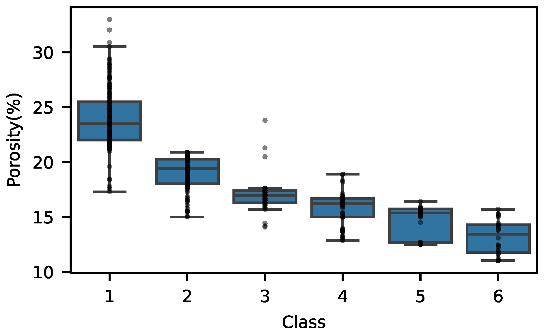
We aim to achieve complementary perspectives between the two models through collaborative training. In this paper, we focus on realizing perspective complementarity between the two tasks during the second training stage using dataset $D_{diff}$. Unlike the standard co-training assumption, the two models are designed for different tasks and predict distinct parameters; thus, establishing a relationship between them is particularly important. The most straightforward approach would be to use empirical formulas to relate the two parameters. However, this approach is limited by the difficulty of obtaining accurate mappings between the two physical parameters, as their relationships often vary across logging conditions due to geological differences. By classifying permeability levels in Table 1, the relationships between permeability and porosity for different categories are illustrated in Figure 5.

We observe a positive correlation between porosity and the reservoir type. Because of the risks associated with inaccurate numerical estimations from empirical formulas, we adopt a distance-based interval probability method to establish the connection between porosity and reservoir type:

$$P_r^{\left(k\right)}={\displaystyle \frac{\exp \left(-\frac{\left|f_1\left(x\right)-{\mu }_k\right|}{2\tau }\right)}{{\sum }_{i=1}^6\exp \left(-\frac{\left|f_1\left(x\right)-{\mu }_i\right|}{2\tau }\right)}}$$

(5)

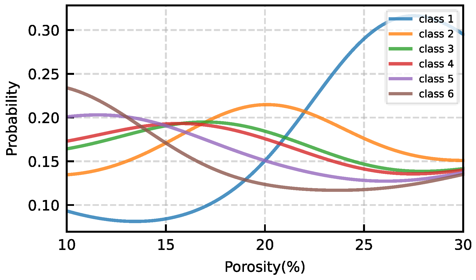
where ${\mu }_i$ is the midpoint of the interval for reservoir type $i$, to ensure statistical robustness against outliers inherent in well-log measurements, ${\mu }_i$ is strictly defined as the median value derived from the boxplot analysis of the porosity distribution within that specific class. and $\tau$ is the temperature coefficient that controls the steepness of the probability distribution, and $P_r^{\left(k\right)}$ denotes the transformed probability that the sample belongs to the reservoir type. Figure 6 demonstrates the transformation of porosity into a probability distribution when the temperature coefficient $\tau$ = 1.

This paper proposes a conditional mask–based category-aware loss based on JS divergence. In our task, the porosity prediction is transformed into a probability distribution using a predefined formula. While consistency between porosity and permeability predictions is expected, the category probabilities derived from the formula-based conversion may differ from the probability distribution directly output by the model. Furthermore, as shown in Figure 5, a specific porosity value does not necessarily correspond to a single reservoir category. For instance, a porosity value of 15% may correspond to either reservoir type 4 or type 5. While the transformed probability distribution reflects the likelihood of each category, both type 4 and type 5 predictions are valid for such a sample. Therefore, this factor must be incorporated when calculating discrepancies between probability distributions. We designed a conditional mask whose construction strategy explicitly accounts for this phenomenon. The definition of the dynamic conditional mask is based on the following two considerations:

$$M_{disagreement}=\{\begin{array}{c}1,argmax\left(P_1\right)\ne argmax\left(P_2\right)\\ 0,argmax\left(P_1\right)=argmax\left(P_2\right)\end{array}$$

(6)

$$M_{weight}=abs\left(argmax\left(P_1\right)-argmax\left(P_2\right)\right)$$

(7)

where $P_1$ represents the converted probability distribution from Model 1’s porosity prediction, $P_2$ represents the probability distribution directly output by Model 2’s classification branch. $M_{disagreement}$ represents the explicit divergence captured between the prediction results of the two branches. If the predictions of both models already align for a given sample, the difference is not computed to mitigate potential impacts on model training. $M_{weight}$ calculates a weighting scheme to assign a tolerance value to the divergence. This design allows the loss function to penalize predictions with large discrepancies while tolerating smaller ones. Multiplying $M_{disagreement}$ and $M_{weight}$ yields the conditional mask matrix. Based on the resulting mask, we construct an optimization objective loss function using JS divergence:

$$\{\begin{array}{c}{M}_{condition}=M_{disagreement}⨀M_{weight}\\ L_{JS-CMSL}=\left[H\left({\displaystyle \frac{P_1+P_2}{2}}\right)-{\displaystyle \frac{H\left(P_1\right)+H\left(P_2\right)}{2}}\right]⨀M_{condition}\end{array}$$

(8)

Here, $H(·)$ denotes information entropy, and $L_{JS-CMCL}$ is the final loss function, which imposes consistency constraints only in the regions indicated by the mask. In addition, for dataset $D_{diff}$, this part of the data only has one label marked, either porosity or permeability, with the other label missing. Furthermore, for dataset $D_{diff}$, only one of the porosity or permeability labels is present, with the other label being missing. Therefore, we employ this loss function to facilitate complementary perspectives between the two models within dataset $D_{diff}$ and to train on the unlabeled dataset $U$.

We drive consistency and complementary perspectives between the two models by employing shape context–based data augmentation techniques and training processes that utilize unlabeled data. Furthermore, we aim to enhance sample diversity and model robustness through generative modeling approaches. Given that reservoir parameter prediction data typically exhibit small-scale, human-indistinguishable features, generative networks such as GANs and diffusion models struggle to control the quality of generated samples. Therefore, this paper employs FGSM (Fast Gradient Signed Method) to generate adversarial samples. FGSM generates adversarial samples by adding a controllable, minimal perturbation to the original input data, guiding the model toward increased loss values. Unlike Gan and diffusion models, FGSM does not generate new data from scratch; It uses a disturbance $ϵ$ and applies it directly to actual seismic data. This bounded perturbation safely expands the local sample diversity and strictly verifies the robustness of the framework in the cross-validation process. We generate adversarial examples from a labeled dataset. To mitigate potential adverse effects on the model, we employ a cross-validation strategy for adversarial sample generation with random perturbations. For each sample generation, we randomly perturb a subset of the model’s parameters to ensure uniqueness among FGSM-generated samples. Additionally, we cross-validate the reliability of all generated adversarial samples. We aim for generated samples to be adversarial and enhance model robustness; however, excessive perturbations can cause destructive effects and contaminate the dataset. For a sample generated via Model 1, we first require that its input to Model 1 yields unchanged predictions, thereby preventing overly disruptive perturbations. Additionally, we require that its input to Model 2 yields different results from those of Model 1, ensuring that the perturbations are effective. This approach allows us to control perturbation intensity within reasonable bounds. These two strategies collectively enrich both the input space and the feature space. Incorporating unlabeled data enhances exposure to diverse geological feature patterns, whereas integrating adversarial examples strengthens robust representation learning. Their combination significantly improves the stability and generalization capabilities of the proposed semi-supervised framework. After specifying the loss functions for the three stages, the final loss is shown below:

$$L=L_{sup}+\lambda L_{JS-CMCL}$$

(9)

where $\lambda$ is a hyperparameter set in advance.

3. Results

The proposed method was evaluated using real data. The study area is located in the South China Sea region. This area has a limited number of logging wells with irregular distribution, and there is a significant lack of parameter data, particularly permeability data. Several issues remain, including a limited understanding of distribution patterns, an unclear reservoir formation process, complex petrophysical relationships, insufficient understanding of gas–water reservoir states, and difficulties in evaluating productivity and dynamic reserves. We designed three sets of experiments: (1) using samples located at the center of the window for STP prediction, (2) incorporating SC into STP prediction, and (3) combining SC and DCT for STP prediction; hereinafter, these approaches are referred to as STP, SC-STP, and DCT–SC–STP, respectively. STP uses a convolutional neural network with residual blocks, with inputs consisting of original seismic data and seismic attribute data extracted using commercial software. The other two experiments additionally incorporate a network structure of the same depth, with shape context as input, which is ultimately output through a fusion layer.

We allocated 80% of the logging sample points to the training set $D_{train}$ and the remaining 20% to the testing set $D_{test}$. In the two experiments that included the shape context descriptor, we performed random resampling within the training set $D_{train}$ using a sliding window. In contrast, for the experiment without the shape context descriptor, the extracted data consisted of a three-dimensional window centered on the sample points of $D_{test}$.

Table 2. The number of datasets used in this article.

Sample Number	Dataset
916	$D_1$
684	$D_2$
232	$D_{diff}$
5000	$U$
3940	$D_{train}$

summarizes the data distribution used in our experiments. To simulate a realistic semi-supervised scenario, $D_1$ (916 samples) serves as the primary labeled dataset, which is further partitioned into $D_2$ (684 samples) and $D_{diff}$ (232 samples) to provide distinct data perspectives for the dual-task co-training branches. Additionally, a large unlabeled seismic dataset $U$ (5000 samples) is incorporated to exploit the vast potential of unlabeled information. The final training set $D_{train}$ (3940 samples) will be divided into training sets at the intersection of $D_1$ and $D_2$, and then randomly expanded with a larger number of samples. Additionally, three wells were retained as validation wells. In this paper, the network model is a convolutional neural network (CNN) incorporating skip connections. The input seismic data have a dimension of 3 × 3 × 13, and the learning rate is set to 0.01. The model is trained for 600 epochs using a 3 × 3 × 3 3D convolution kernel for seismic data and a 3 × 3 convolution kernel for shape context.

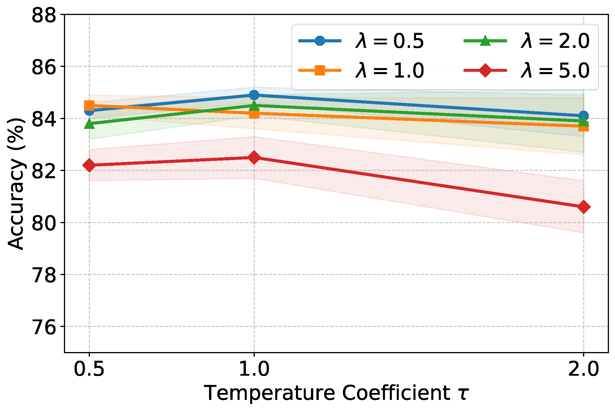
The hyperparameters selected in this article are $\lambda$ = 0.5 and $\tau$ = 1. As mentioned earlier, $\lambda$ is the weight of the $L_{JS-CMCL}$, and $\tau$ is the temperature coefficient of the probability map. Since the labeled samples for permeability (reservoir type) are strictly a subset of the porosity samples, the classification branch, in the absence of direct supervision signals, relies heavily on the cross-task consistency loss ($L_{JS-CMCL}$) to incorporate complementary information. Consequently, the classification performance exhibits a higher sensitivity to variations in the hyperparameters of this loss function. To address this, we focused our cross-sensitivity analysis on the impact of the loss weight $\lambda$ and the temperature coefficient $\tau$ on the accuracy of the classification model, with the results illustrated in Figure 7.

The results indicate that the model achieves its peak classification accuracy at $\tau$ = 1.0. Deviating from this optimal value (e.g., 0.5 or 2.0) leads to a slight decrease in performance, demonstrating that an appropriate temperature coefficient is necessary to prevent the probability distribution from becoming overly sharp or too flat. More importantly, the accuracy curves for $\tau$ = 0.5, 1.0, and 2.0 are tightly clustered with overlapping standard deviations. This clearly demonstrates that our proposed framework is highly robust and relatively insensitive to the consistency loss weight within the broad range of [0.5, 2.0]. However, an excessively large weight ($\tau$ = 5.0) significantly degrades performance, as the consistency constraint begins to overwhelm the primary supervised learning tasks. Based on these empirical findings, we set $\tau$ = 1 and $\lambda$ = 1 for all subsequent experiments.

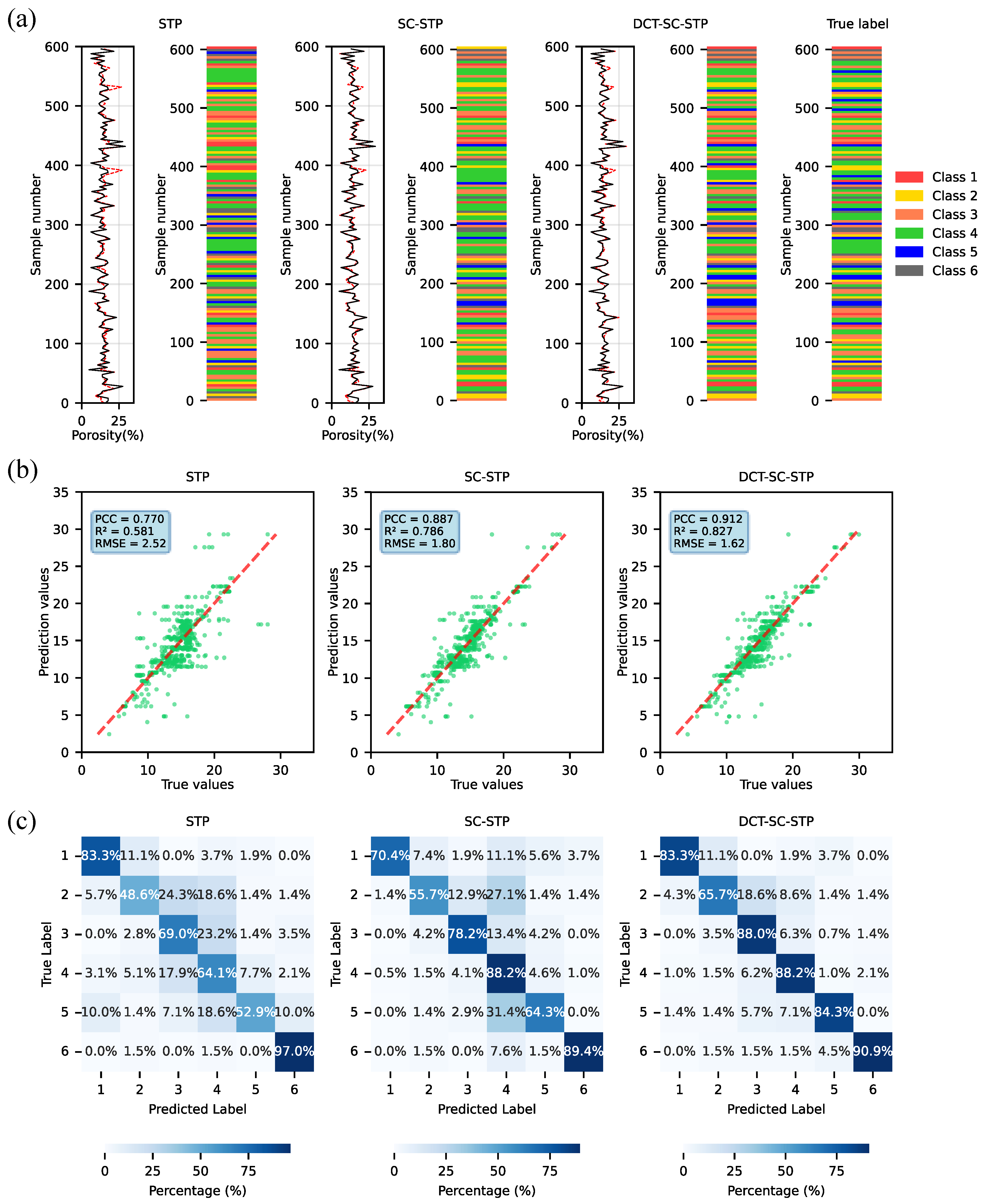
Figure 8 shows the predictive performance of three methods on the test dataset from multiple perspectives, including curve comparison, classification prediction accuracy, and quantitative regression consistency.

Figure 8a shows the porosity prediction curve and corresponding reservoir type classification results. In the porosity curve graph, the black solid line represents the true porosity value obtained from well logging records, while the red dashed line represents the predicted porosity generated by the model. By comparing the predicted curve with the true value, it can be observed that the basic STP model shows significant deviations in several depth intervals, especially near areas where porosity values change rapidly. After introducing Shape Context Descriptors (SC-STP), the predicted curve became more closely aligned with the overall trend of true porosity, indicating that shape context descriptors effectively enhance the model’s ability to capture waveform morphology and local structural features in seismic records. When the dual task deep collaborative training framework (DCT–SC–STP) is further introduced, the consistency between the predicted porosity curve and reservoir type reaches the highest level. This improvement indicates that collaborative learning between regression and classification tasks helps the model better utilize the complementary information contained in the data.

Figure 8b shows the scatter plots of predicted porosity and true porosity values using three methods. Ideally, the predicted value should be closely aligned with the diagonal, representing a perfect prediction. As shown in the figure, the distribution of STP predicted values is relatively scattered, significantly deviating from the diagonal, reflecting a large prediction error. After introducing shape context descriptors, the SC-STP results are more concentrated near the diagonal, indicating an improvement in regression accuracy. The DCT–SC–STP method further tightened the distribution of points near the diagonal and showed the smallest prediction error among the three methods. This result confirms that the proposed framework effectively improves regression performance by integrating structural information of seismic waveforms and utilizing complementary learning between porosity prediction and reservoir classification.

Figure 8c shows the confusion matrix of three methods for predicting reservoir types. The confusion matrix quantitatively evaluates classification performance by comparing predicted categories with real labels. Compared with the STP model, SC-STP and DCT–SC–STP have higher values on diagonal elements, indicating an improvement in classification accuracy. Especially, the DCT–SC–STP method has a more concentrated distribution on the diagonal and fewer misclassifications between adjacent reservoir types. This result indicates that the combination of shape context descriptors and dual task collaborative training effectively enhances the model’s ability to distinguish different reservoir categories.

Table 3. Quantitative comparison of predictive performance of three experiments.

Method	PCC	R2	RMSE	Accuracy
STP	0.770	0.581	2.52	0.712
SC-STP	0.887	0.786	1.80	0.801
DCT–SC–STP	0.912	0.827	1.62	0.849

presents the quantitative evaluation results of the STP, SC-STP, and our proposed DCT–SC–STP framework on the test set. It is evident that the step-by-step integration of our designed modules progressively and significantly enhances the predictive performance for both porosity regression and reservoir type classification.

Table 4. Training duration for three experiments (100 epochs).

Method	Training Time (min/100 epoch)
STP	14.76
SC-STP	16.5
DCT–SC–STP	24.25

shows the comparison of training time between STP, SC-STP, and our proposed DCT–SC–STP framework. We record the time every 100 epochs and calculate the average. This training time is the result of parallel training of the two models. It can be seen that adding SC and DCT requires more time overhead. We believe that the trade-off between accuracy and computational cost is acceptable.

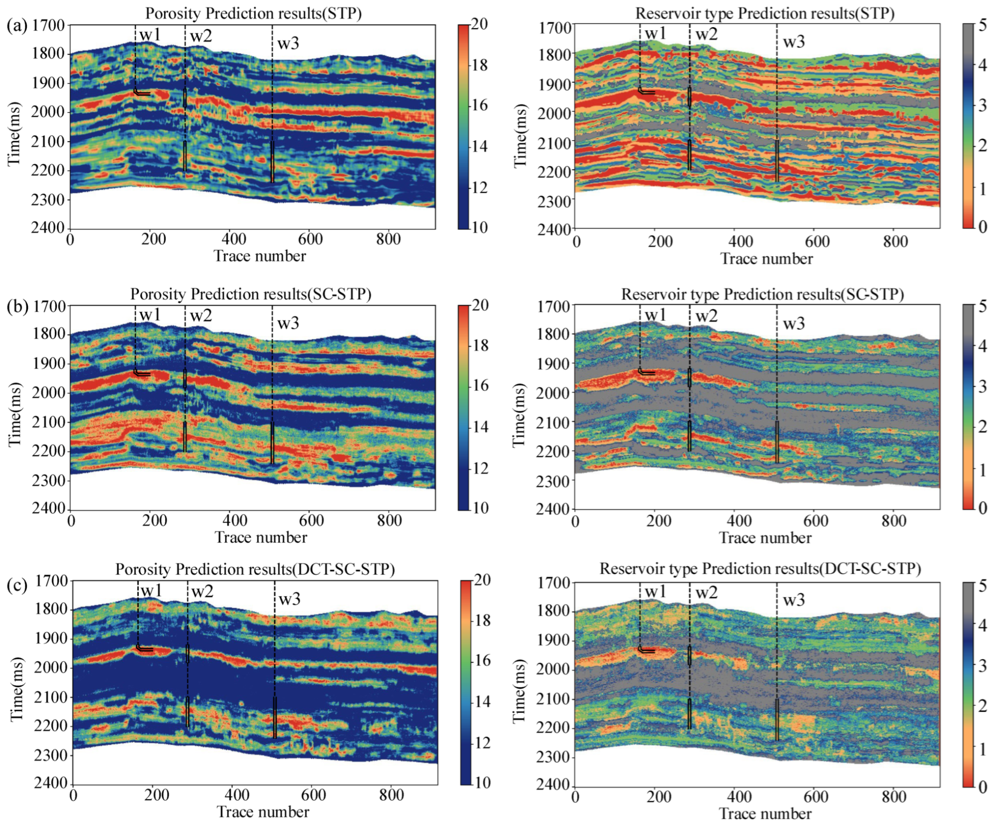
After validation on the test set, we further conducted predictions on seismic profiles, as shown in Figure 9. We performed predictions on the combined profile of three blind wells, where W1, W2, and W3 denote the three blind wells. Figure 9a shows the STP prediction results, Figure 9b shows the SC-STP prediction results, and Figure 9c shows the DCT–SC–STP prediction results. The left side displays the porosity profile prediction results, whereas the right side shows the reservoir type profile prediction results. Compared to STP, SC-STP predictions exhibit superior lateral continuity. At Well W2 (highlighted by the red oval), STP exhibits poorer lateral continuity and displays vertical strip-like patterns. This situation occurs because the STP prediction paradigm struggles to capture variations in seismic data within fixed windows, whereas the SC-STP method incorporates seismic waveform information to enhance lateral continuity in predictions. Regarding reservoir type predictions, STP tends to overestimate reservoir types and fails to clearly delineate boundaries, with profile predictions exhibiting chaotic downhole phenomena. This indicates that the STP prediction paradigm struggles to accurately delineate favorable target zones. SC-STP more precisely delineates reservoir boundaries in its predictions. However, combining the SC-STP’s porosity and reservoir-type profiles reveals discrepancies at well W3 (highlighted by the red circle). While reservoir-type predictions align well with labels in the upper half of W3, the porosity results show opposite trends. The lack of consistency between tasks makes it difficult to determine whether the area constitutes a favorable reservoir. By leveraging the complementary perspectives of both models through a co-training framework, the DCT–SC–STP predictions demonstrate strong inner-task consistency. The porosity prediction profile at W3 aligns well with the conclusions drawn from the well data, thereby validating the effectiveness of the co-training approach.

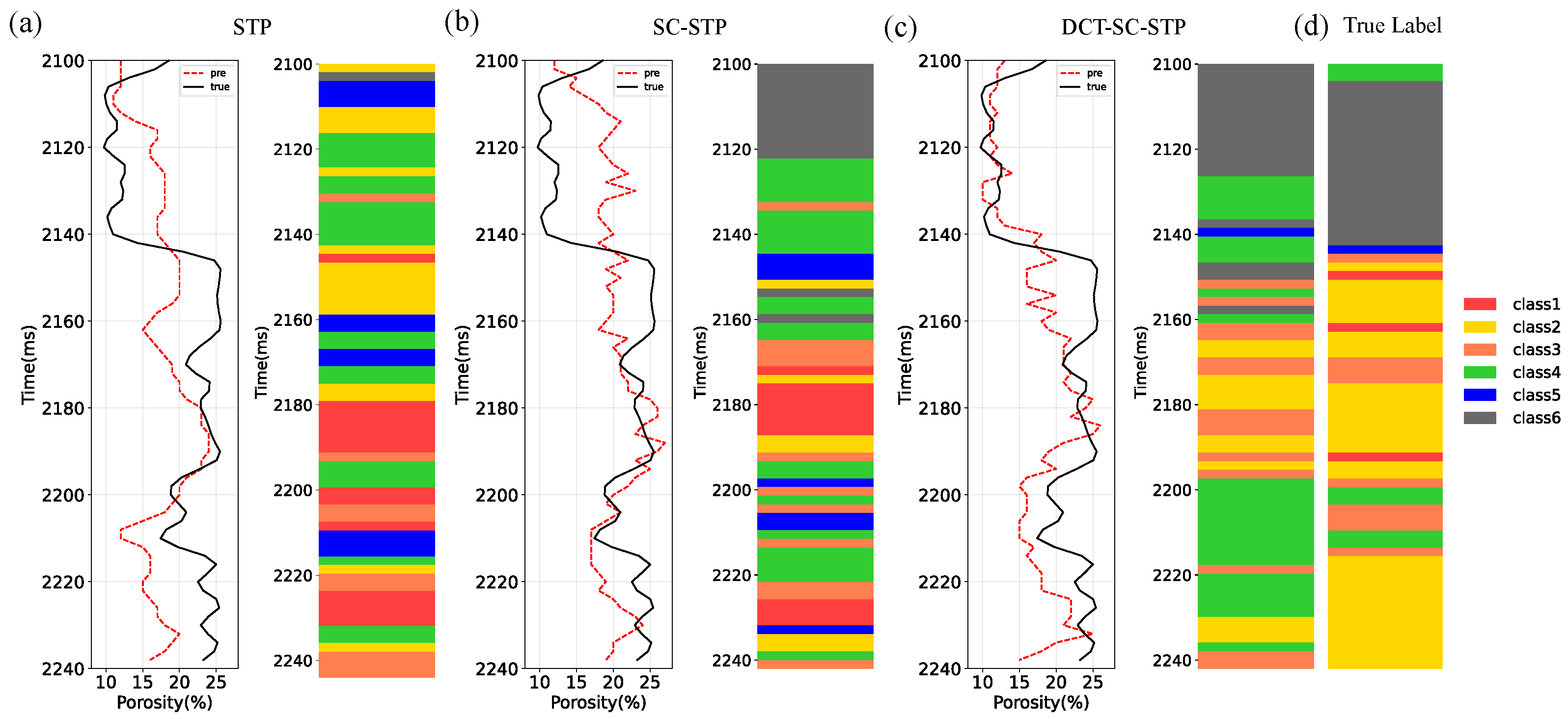
Figure 10 presents the prediction results for blind well W3. Figure 10a shows the STP prediction results, Figure 10b shows the SC-STP prediction results, Figure 10c shows the DCT–SC–STP prediction results, and Figure 10d shows the actual reservoir type labels. The overall trend of the STP porosity prediction results is more gradual, whereas SC-STP exhibits steeper variations. This behavior is attributed to the shape context incorporating the relative position of the target point within the window, enabling the network to more readily extract features at the target location. Overall, DCT–SC–STP demonstrates superior consistency and complementarity, exhibiting greater restraint in predicting high-porosity and high reservoir types. This aids in narrowing the scope of the target area.

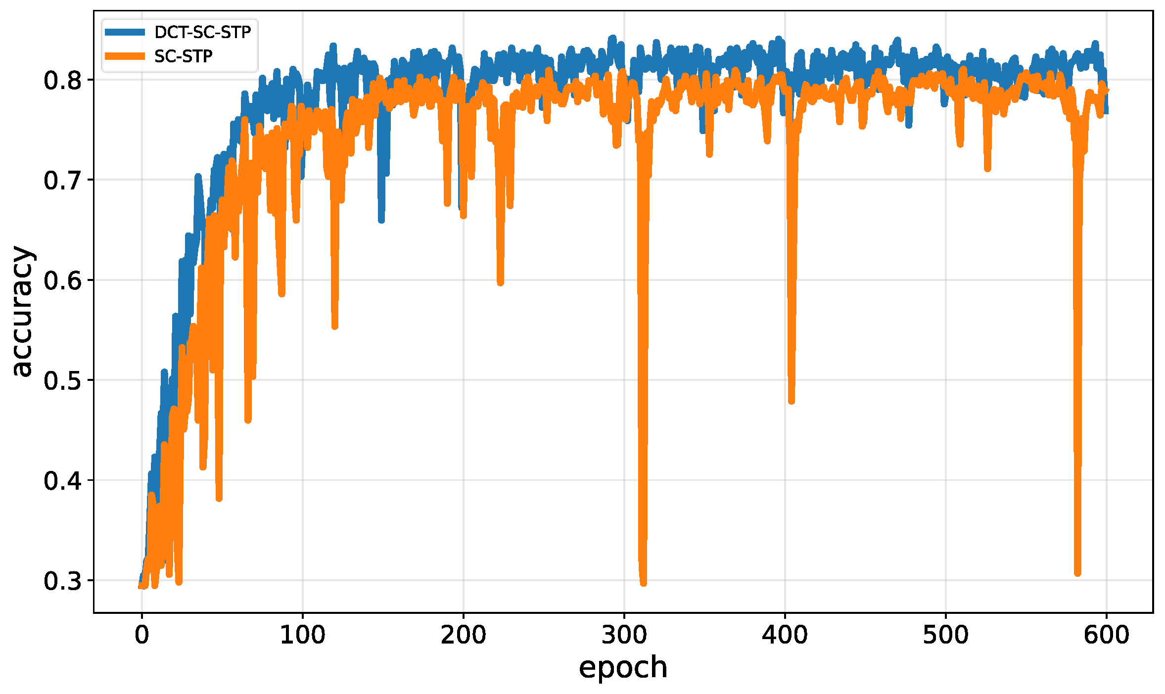
Additionally, we recorded the accuracies of SC-STP and DCT–SC–STP on the test set, as shown in Figure 11. The orange curve represents the accuracy curve for SC-STP, and the blue curve represents the accuracy curve for DCT–SC–STP. We employed 600 epochs, with all other parameters held constant. It is evident that DCT–SC–STP not only achieves higher accuracy but also demonstrates significantly improved training stability, thereby reducing instances of substantial accuracy fluctuations. This enhancement in model stability, attributed to the incorporation of adversarial examples, validates the effectiveness of the adversarial techniques.

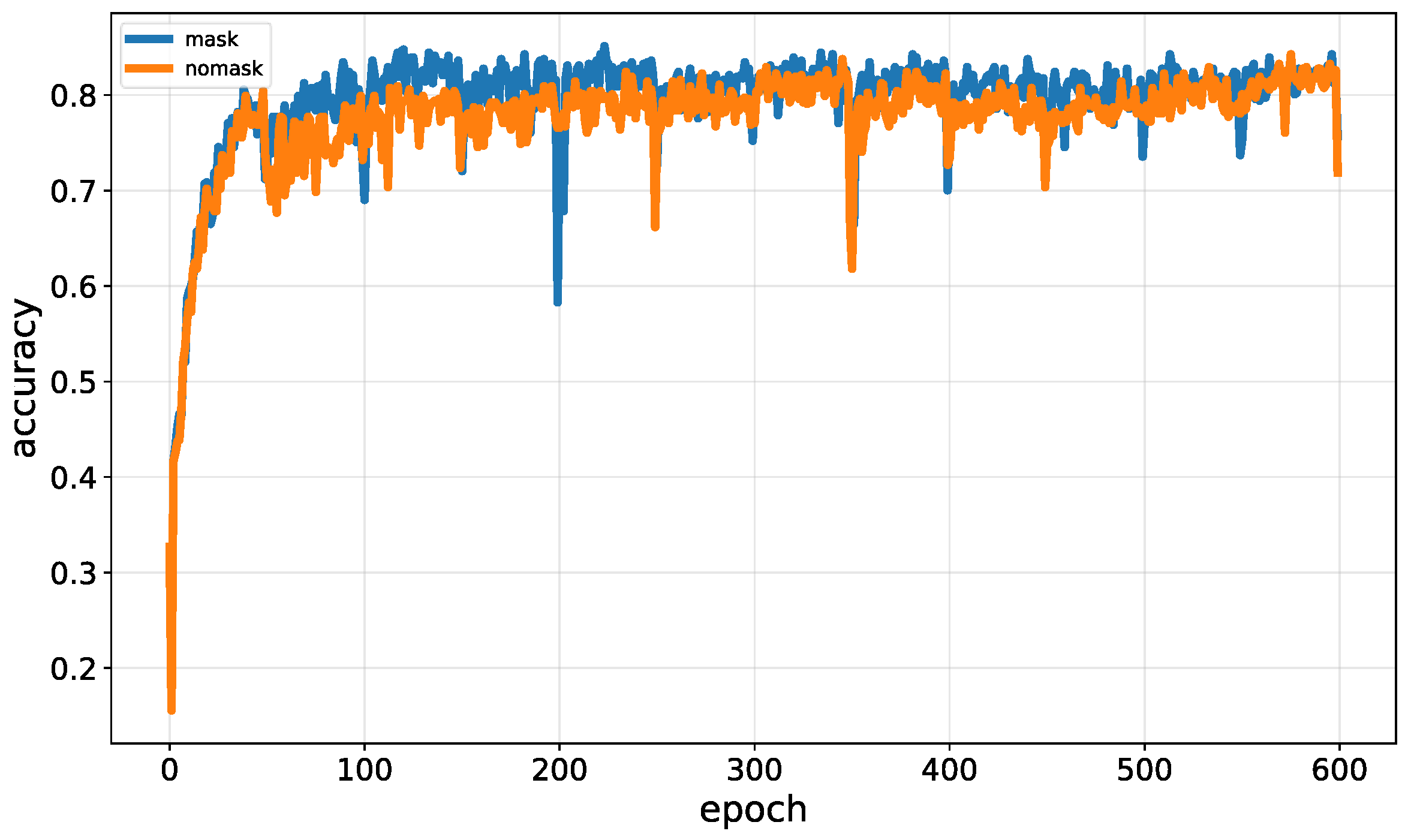
To further illustrate the dynamic impact of the conditional mask during the optimization process, Figure 12 plots the validation accuracy curves over 600 training epochs for both the “Mask” (proposed) and “No Mask” configurations. In contrast, the integration of our proposed conditional mask (blue line) acts as an effective gradient filter. It successfully shields the network from these disruptive signals, leading to a significantly more stable optimization trajectory and ultimately converging at a higher accuracy plateau. This demonstrates that the conditional mask ensures the stability of the dual-task co-training framework.

To rigorously evaluate the proposed DCT–SC–STP framework, we compared it against two representative semi-supervised paradigms: Mean Teacher (MT) and single-task deep co-training (DCT single task). Crucially, to ensure a fair comparison within our dual-task scenario, we implemented task-specific variants for both baselines. That is, we trained independent models for porosity regression (MT-Reg, DCT-Reg) and reservoir type classification (MT-Cls, DCT-Cls).

As presented in

Table 5. Quantitative comparison of the proposed DCT–SC–STP framework with state-of-the-art semi-supervised baselines.

Method	PCC	R2	RMSE	Accuracy
DCT (Single task)	0.876	0.779	1.84	0.798
Mean Teacher	0.891	0.783	1.78	0.807
DCT–SC–STP	0.912	0.827	1.62	0.849

, we quantitatively compared our proposed DCT–SC–STP framework with two representative semi-supervised learning baselines: single-task deep co-training (DCT) and Mean Teacher. Both the single-task DCT and the Mean Teacher struggle to optimize the regression task further. This limitation arises because these traditional paradigms enforce consistency strictly within an isolated continuous space, making them highly susceptible to confirmation bias and lacking explicit constraints on unlabeled data. In contrast, our DCT–SC–STP framework achieves the best overall performance, reducing the porosity RMSE to 1.62 and improving the permeability classification accuracy to 84.9%. This substantial performance margin is primarily attributed to our proposed heterogeneous cross-task consistency mechanism. By projecting continuous regression outputs into a probability space via the mid-point mapping, it safely overcomes the bottlenecks of isolated single-task learning and fully exploits the potential of unlabeled seismic data.

4. Discussion

The proposed DCT–SC–STP framework improves reservoir prediction under limited labeled data through three key mechanisms: shape context encoding, data expansion, and asymmetric dual-task co-training.

The shape context descriptor explicitly encodes relative spatial distributions within seismic sequences, capturing waveform morphology beyond raw amplitudes. This structural information enhances the network’s sensitivity to subtle seismic variations associated with different reservoir properties. The sliding-window expansion strategy mitigates the small-sample problem by generating diverse training samples around each logging point while preserving geological continuity—a critical requirement for seismic data. The asymmetric dual-task framework formulates porosity regression and permeability classification collaboratively, using a conditional mask–based consistency loss. This design captures underlying correlations between the two properties without enforcing rigid empirical relationships, which often vary across geological settings. Furthermore, the integration of unlabeled seismic data via deep co-training, combined with FGSM-based adversarial sample generation, improves model robustness and generalization.

Despite these advantages, several limitations remain. First, the predefined permeability classification intervals simplify learning but may cause information loss compared with direct quantitative prediction. Future work could explore probabilistic regression or multi-task learning for continuous properties. Second, the shape context descriptor focuses on local waveform geometry within a fixed window and may not fully capture larger-scale structures (e.g., faults, stratigraphic boundaries). Incorporating multi-scale representations or structural geological constraints could further improve accuracy and interpretability. Finally, although the method performs well in the study area (Yinggehai Basin), its generalization to other basins with different reservoir characteristics requires validation on diverse datasets.

Overall, integrating shape-based seismic descriptors with semi-supervised dual-task learning offers a promising direction for reservoir prediction in data-limited scenarios, enhancing prediction accuracy, spatial consistency, and model robustness.

5. Conclusions

In this study, an asymmetric deep co-training framework integrated with a shape context descriptor was proposed to improve reservoir property prediction under limited labeled data conditions. The shape context descriptor was introduced to encode the morphological characteristics and spatial relationships of seismic waveforms, thereby enhancing the model’s ability to capture structural features in the STP prediction paradigm. A sliding-window–based data expansion strategy was further employed to alleviate the small-sample problem by increasing the diversity of training samples while preserving geological continuity.

To exploit complementary information between reservoir properties, a dual-task deep co-training framework was designed, in which porosity was predicted through regression while permeability information was incorporated through reservoir-type classification. By introducing a conditional mask–based consistency loss and utilizing unlabeled seismic data, the proposed framework enables collaborative learning between the two tasks and improves model robustness.

Experiments conducted on real seismic data from the South China Sea demonstrate that the proposed DCT–SC–STP method achieves better prediction accuracy, spatial continuity, and classification consistency than baseline approaches. These results indicate that combining shape-based seismic descriptors with semi-supervised dual-task learning provides an effective strategy for reservoir prediction in data-limited scenarios.

References

1. Azevedo, L.; Nunes, R.; Soares, A.; Neto, G.S.; Martins, T.S. Geostatistical seismic Amplitude-versus-angle inversion. Geophys. Prospect. 2018, 66, 116–131. [Google Scholar] [CrossRef]
2. Liu, M.; Grana, D. Stochastic Nonlinear Inversion of Seismic Data for the Estimation of Petroelastic Properties Using the Ensemble Smoother and Data Reparameterization. Geophysics 2018, 83, M25–M39. [Google Scholar] [CrossRef]
3. Wang, J.; Cao, Y.; Liu, K.; Liu, J.; Kashif, M. Identification of Sedimentary-Diagenetic Facies and Reservoir Porosity and Permeability Prediction: An Example from the Eocene Beach-Bar Sandstone in the Dongying Depression, China. Mar. Pet. Geol. 2017, 82, 69–84. [Google Scholar] [CrossRef]
4. Ali Ahmadi, M.; Zendehboudi, S.; Lohi, A.; Elkamel, A.; Chatzis, I. Reservoir Permeability Prediction by Neural Networks Combined with Hybrid Genetic Algorithm and Particle Swarm Optimization. Geophys. Prospect. 2013, 61, 582–598. [Google Scholar] [CrossRef]
5. Zhao, W.; Zhang, Z.; Liao, J.; Zhang, J.; Zhang, W. Prediction Method for the Porosity of Tight Sandstone Constrained by Lithofacies and Logging Resolution. Mar. Pet. Geol. 2024, 170, 107114. [Google Scholar] [CrossRef]
6. Liu, J.; Zhao, L.; Xu, M.; Zhao, X.; You, Y.; Geng, J. Porosity Prediction from Prestack Seismic Data via Deep Learning: Incorporating a Low-Frequency Porosity Model. J. Geophys. Eng. 2023, 20, 1016–1029. [Google Scholar] [CrossRef]
7. Buland, A.; Landrø, M. The Impact of Common-offset Migration on Porosity Estimation by AVO Inversion. Geophysics 2001, 66, 755–762. [Google Scholar] [CrossRef]
8. Li, J.X.; Zhang, T.; Zhu, Y.; Chen, Z. Artificial General Intelligence for the Upstream Geoenergy Industry: A Review. Gas Sci. Eng. 2024, 131, 205469. [Google Scholar] [CrossRef]
9. Liu, D.; Wang, W.; Wang, X.; Wang, C.; Pei, J.; Chen, W. Poststack Seismic Data Denoising Based on 3-D Convolutional Neural Network. IEEE Trans. Geosci. Remote Sens. 2020, 58, 1598–1629. [Google Scholar] [CrossRef]
10. Zhu, Y.; Cao, J.; Yin, H.; Zhao, J.; Gao, K. Seismic Data Reconstruction Based on Attention U-Net and Transfer Learning. J. Appl. Geophys. 2023, 219, 105241. [Google Scholar] [CrossRef]
11. Hami-Eddine, K.; Klein, P.; Richard, L.; De Ribet, B.; Grout, M. A New Technique for Lithology and Fluid Content Prediction from Prestack Data: An Application to a Carbonate Reservoir. Interpretation 2015, 3, SC19–SC32. [Google Scholar] [CrossRef]
12. Nie, W.; Gu, J.; Li, B.; Wen, X.; Nie, X. Quantitative Lithology Prediction from Seismic Data Using Deep Learning. Comput. Geosci. 2025, 196, 105821. [Google Scholar] [CrossRef]
13. Pan, X.; Li, X.; Huang, L.; Li, L.; Wang, P.; Liu, J. Estimation of Fracture Properties from Azimuthal Seismic Data Using Convolution Neural Network. IEEE Geosci. Remote Sens. Lett. 2024, 21, 3002005. [Google Scholar] [CrossRef]
14. Bönke, W.; Alaei, B.; Torabi, A.; Oikonomou, D. Data Augmentation for 3D Seismic Fault Interpretation Using Deep Learning. Mar. Pet. Geol. 2024, 162, 106706. [Google Scholar] [CrossRef]
15. Yin, L.; Xu, J.; Du, Q.; Zhang, G.; Qi, X.; Tang, Y. Marine Geomechanical Approach to Well Trajectory Optimization in Fractured Reservoirs: A Case Study from the X Block, Zhujiangkou Basin. J. Mar. Sci. Eng. 2025, 13, 1732. [Google Scholar] [CrossRef]
16. Gui, J.; Gao, J.; Li, S.; Liu, B.; Chen, Q. A Deep Learning Framework for Petrophysical Properties Prediction in Gas Reservoirs. IEEE Geosci. Remote Sens. Lett. 2024, 21, 7508405. [Google Scholar] [CrossRef]
17. Isa, A.D.; Gebretsadik, H.T.; Muhammad, A.; Mohammed, H.S.; Kurah, I.M.; Salisu, A.K. Porosity Estimation Using Deep Learning and ImageJ: Implications for Reservoir Characterization in Central Luconia Miocene Carbonates. Mar. Pet. Geol. 2025, 182, 107538. [Google Scholar] [CrossRef]
18. Zhang, Y.; Fan, C.; Qin, D.; Wang, X.; Jiang, B. Deep-Learning-Based Prediction of Mutant Formation Pore Pressure: A Case Study from the Xihu Sag in the East China Sea. Gas Sci. Eng. 2026, 147, 205846. [Google Scholar] [CrossRef]
19. Tao, L.; Gu, Z.; Ren, H. Improving the Seismic Impedance Inversion by Fully Convolutional Neural Network. J. Mar. Sci. Eng. 2025, 13, 262. [Google Scholar] [CrossRef]
20. Ao, Y.; Lu, W.; Hou, Q.; Jiang, B. Sequence-to-Sequence Borehole Formation Property Prediction via Multi-Task Deep Networks with Sparse Core Calibration. J. Pet. Sci. Eng. 2022, 208, 109637. [Google Scholar] [CrossRef]
21. Xu, M.; Zhao, L.; Liu, J.; Geng, J. Enhancing Seismic Porosity Estimation through 3D Sequence-to-Sequence Deep Learning with Data Augmentation, Spatial Constraints, and Geologic Constraints. Geophysics 2024, 89, M93–M108. [Google Scholar] [CrossRef]
22. Xu, P.; Lu, W.; Wang, B. A Semi-Supervised Learning Framework for Gas Chimney Detection Based on Sparse Autoencoder and TSVM. J. Geophys. Eng. 2019, 16, 52–61. [Google Scholar] [CrossRef]
23. Geng, Z.; Hu, Z.; Wu, X.; Liang, L.; Fomel, S. Semisupervised Salt Segmentation Using Mean Teacher. Interpretation 2022, 10, SE21–SE29. [Google Scholar] [CrossRef]
24. Dou, Y.; Li, K.; Lv, W.; Li, T.; Xiao, Y. ContrasInver: Ultra-Sparse Label Semi-Supervised Regression for Multidimensional Seismic Inversion. IEEE Trans. Geosci. Remote Sens. 2024, 62, 5917613. [Google Scholar] [CrossRef]
25. Lin, G.; Jiang, J.; Bai, J.; Su, Y.; Su, Z.; Liu, H. Frontiers and Developments of Data Augmentation for Image: From Unlearnable to Learnable. Inf. Fusion 2025, 114, 102660. [Google Scholar] [CrossRef]
26. Wu, N.; Wang, Y.; Li, Y. Noise Suppression of Distributed Fiber-Optical Acoustic Sensing Seismic Data by Attention-Guided Multiscale Generative Adversarial Network. Geophysics 2023, 88, D227–D239. [Google Scholar] [CrossRef]
27. Luo, X.; Sun, J.; Zhang, R.; Chi, P.; Cui, R. A Multi-Condition Denoising Diffusion Probabilistic Model Controls the Reconstruction of 3D Digital Rocks. Comput. Geosci. 2024, 184, 105541. [Google Scholar] [CrossRef]
28. Lee, D.; Ovanger, O.; Eidsvik, J.; Aune, E.; Skauvold, J.; Hauge, R. Latent Diffusion Model for Conditional Reservoir Facies Generation. Comput. Geosci. 2025, 194, 105750. [Google Scholar] [CrossRef]
29. Shi, Z.; Tang, X.; Pang, S.; Chi, Y. Prestack gather residual moveout correction based on shape context and dynamic time warping. Lithol. Reserv. 2017, 29, 113–119. [Google Scholar] [CrossRef]
30. Nie, F.; Wei, Y.; Zheng, Y.; Deng, H. Study on Deep Learning of Ore-Controlling Characteristics of Geological Morphology and 3D Metallogenic Prediction Based on Shape Context—A Case Study of Dayingezhuang Gold Deposit. Adv. Geosci. 2021, 11, 137–146. [Google Scholar] [CrossRef]
31. Zheng, L.; Yang, H.; Luo, G. Seismic Waveform Feature Extraction and Reservoir Prediction Based on CNN and UMAP: A Case Study of the Ordos Basin. Appl. Sci. 2025, 15, 7377. [Google Scholar] [CrossRef]
32. Belongie, S.; Malik, J.; Puzicha, J. Shape Matching and Object Recognition Using Shape Contexts. IEEE Trans. Pattern Anal. Mach. Intell. 2002, 24, 509–522. [Google Scholar] [CrossRef]
33. Shah, M.P.; Singha, S.; Awate, S.P. Leaf Classification Using Marginalized Shape Context and Shape+texture Dual-Path Deep Convolutional Neural Network. In Proceedings of the 2017 IEEE International Conference on Image Processing (ICIP); IEEE: Beijing, China, 2017; pp. 860–864. [Google Scholar]
34. Xie, S.; Liu, S.; Chen, Z.; Tu, Z. Attentional ShapeContextNet for Point Cloud Recognition. In Proceedings of the 2018 IEEE/CVF Conference on Computer Vision and Pattern Recognition; IEEE: Salt Lake City, UT, USA, 2018; pp. 4606–4615. [Google Scholar]
35. Qiao, S.; Shen, W.; Zhang, Z.; Wang, B.; Yuille, A. Deep Co-Training for Semi-Supervised Image Recognition. In Computer Vision—ECCV 2018; Ferrari, V., Hebert, M., Sminchisescu, C., Weiss, Y., Eds.; Lecture Notes in Computer Science; Springer International Publishing: Cham, Switzerland, 2018; Volume 11219, pp. 142–159. [Google Scholar]
36. SY/T 6285-2011; Method for Reservoir Evaluation of Oil and Gas. Petroleum Industry Press: Beijing, China, 2011.
Figure 1. Workflow of the proposed method for deep co-training of dual models with fused shape contexts, where the orange arrow represents the workflow of one model and the blue arrow represents the workflow of the other model.
Jmse 14 00746 g001
Figure 2. Mapping of single-channel seismic data to polar coordinates.
Jmse 14 00746 g002
Figure 3. Data expansion diagram; (a) expansion method in the horizontal direction; (b) expansion method in the vertical direction.
Jmse 14 00746 g003
Figure 4. Porosity and permeability distribution maps of internal wells in the study work area; (a) porosity distribution map; (b) permeability distribution map.
Jmse 14 00746 g004
Figure 5. Box plot showing the relationship between porosity and reservoir type, with six reservoir types on the horizontal axis and specific porosity values on the vertical axis.
Jmse 14 00746 g005
Figure 6. Probability distribution plots for different porosity mapping strategies.
Jmse 14 00746 g006
Figure 7. Sensitivity analysis of classification accuracy with respect to the temperature coefficient τ under different consistency loss weights λ . The solid lines represent the mean accuracy, and the corresponding colored shaded regions indicate the standard deviation across multiple experimental runs.
Jmse 14 00746 g007
Figure 8. Prediction results of three methods on the test set: (a) porosity and reservoir type prediction results, (b) scatter plot of porosity predictions versus true values, and (c) confusion matrix of reservoir type prediction.
Jmse 14 00746 g008
Figure 9. Profile prediction results of three methods: (a) STP prediction result; (b) SC-STP prediction result; (c) DCT–SC–STP prediction result. W1, W2 and W3 are three blind wells used for validation; the left panel shows the porosity prediction profile, and the right panel shows the reservoir type prediction profile.
Jmse 14 00746 g009
Figure 10. Prediction results of three methods on blind well W3: (a) STP prediction result, (b) SC-STP prediction result, (c) DCT–SC–STP prediction result, and (d) actual reservoir type label. The red dashed line represents the predicted value, and the black solid line represents the actual value.
Jmse 14 00746 g010
Figure 11. Accuracy curves of SC-STP and DCT–SC–STP, with epochs on the x-axis and accuracy on the y-axis.
Jmse 14 00746 g011
Figure 12. Comparison of training accuracy curves for the classification branch with the proposed conditional mask (blue) and without the mask (orange).
Jmse 14 00746 g012