Modeling Wave Energy Dissipation by Bottom Friction on Rocky Shores

Abstract

Rocky shores are characterized by rough, multi-scale bathymetric variations that result in enhanced wave energy dissipation by bottom friction compared to sandy beaches. Realistic SWAN simulations of surface gravity waves across the rocky shores of Monterey (CA, USA) are conducted, and model results are compared to 20 inner-shelf observational sites spanning 34–5 m water depth. The wave field was highly variable during the study, including alternately low energy waves dominated by southern swell and higher energy local waves aligned with strong north-westerly winds. Including a modified bottom friction parameterization is required for the model to reproduce bulk wave statistics with high skill across the entire inner shelf. The SWAN simulation with the default bottom friction parameterization overestimates significant wave height relative to observations because the friction factor $f_e$ parameterization has a maximum value of 0.3. Additional simulations included two empirical formulations relating $f_e$ to the normalized wave excursion $A_b/k_N$ in the large roughness regime $A_b/k_N<1$. Both simulations incorporate a higher $f_e$ that is required to model strong bottom friction dissipation over rocky seabeds. The higher friction factors, with 80% falling within the range 0.43 to 5.38, are associated with variability in the normalized orbital excursion within $0.1<A_b/k_N<1$. This range corresponds to a large bottom roughness length scale, $k_N=0.5$ m, characteristic of rocky shore environments.

1. Introduction

Surface gravity wave transformation across the nearshore is critical to a wide range of applications, including shoreline infrastructure protection, navigation safety, and coastal management (e.g., [1,2,3,4]). Combined with observations, numerical models are used to predict wave evolution across complex coastal environments, where factors such as substrate type, bathymetric slope, and shoreline irregularities can all influence wave transformation. Numerical models must reliably simulate the range of relevant processes governing nearshore wave transformation to effectively support management decisions. For example, well-evaluated and tuned wave dissipation models are needed to assess the benefits of natural or engineered features on shoreline protection [2,3,5,6,7]. Well-evaluated numerical models can also play a key role in filling observational gaps and projecting wave conditions under future scenarios, such as sea-level rise, changes in storm strength and frequency, and reef degradation or restoration [7,8,9,10,11,12]. Recent observations from rough, complex seabeds, such as coral reefs, have begun to inform numerical modeling of these environments (e.g., [13,14,15,16,17,18,19,20,21]).

In the coastal ocean, wave dissipation is an important process that must be accurately represented in numerical models, as it directly affects shoreline exposure to wave energy, wave setup, and wave-driven currents. Common mechanisms for nearshore wave energy dissipation are bottom friction and wave breaking [13,15,22]. On sandy beaches, dissipation is typically dominated by depth-limited wave breaking [22]. In contrast, observational studies of nearshore areas with rough seabeds, such as coral reef (e.g., [13,14,23,24]) or rocky shore (e.g., [15,18,21,25]) environments, suggest that dissipation by bottom friction is enhanced relative to sandy beaches and can equal or exceed dissipation by wave breaking. For example, in a barrier reef system under low-energy conditions ($H_{rms}<0.6$ m), Lowe et al. [23] find bottom friction dissipation exceeds wave breaking by a factor of four. In these environments, enhanced wave energy dissipation by bottom friction and weakened wave breaking can substantially modify coastal dynamics, for example, by reducing the energy available to drive wave-breaking-induced currents in the surf zone, highlighting the importance of accurately representing bottom friction dissipation in coastal models [21,23,26].

From pairs of observations such as buoys or moorings, wave dissipation can be estimated by applying a simplified, discretized steady-state wave energy equation,

$${\displaystyle \frac{\mathsf{\Delta }{F}_x(f,\theta )}{\mathsf{\Delta }x}}=-D_f+ϵ.$$

(1)

Here, the wave energy flux $F_x$ is a function of frequency f and direction $\theta$ with the x coordinate oriented in the direction of a neighboring observation location and $ϵ$ represents neglected processes. A standard parameterization of wave bottom friction dissipation,

$$D_f=A\rho f_e{u}_b^3,$$

(2)

can be used where $\rho$ is seawater density, $u_b$ is seabed wave orbital velocity, and $f_e$ is a wave energy dissipation factor (e.g., [27,28]). The numerical constant A depends on the choice of wave field statistical characterization used to estimate $u_b$ (c.f., Appendix, [21]). for a survey from recent results. Where the simplifications of Equation (1) are satisfied, finite difference estimates of $F_x$ are taken between location pairs, and $f_e$ can be estimated through a fitting procedure between $\mathsf{\Delta }{F}_x(f,\theta )/\mathsf{\Delta }x$ and ${\overline{u_b}}^3$, where $\overline{\phantom{x}}$ denotes a spatial average between instruments. Although calculation details vary between studies, they consistently demonstrate larger $f_e$ in coral reef and rocky shore environments [13,14,15,21,23,24,29,30,31]. With coefficients corrected for Rayleigh wave distributions [25], the reported values of $f_e$ reach 2.5 and 17 on coral reefs and rocky shores, respectively [15,32], both much higher than sandy beach values between ${10}^{-3}$ and ${10}^{-1}$ [33].

The large $f_e$ in coral reef and rocky shore environments is presumed to arise from the presence of rough and complex seabed features with many scales of variability (e.g., [14,15,34]). This complexity is potentially captured by a single length-scale ${\sigma }_b$, defined as the vertical range of seabed elevation or its variability from the mean value [35]. These same seabed features, such as individual coral heads or rocks and mounds, are typically small relative to surface gravity wave lengths and are therefore unresolved by regional wave-averaged numerical models. Within this bottom roughness framework, several empirical and theoretical models relate ${\sigma }_b$ to wave friction factor $f_e$ through the non-dimensional ratio $A_b/{\sigma }_b$ (e.g., [28,36]) where $A_b$ is the wave orbital excursion. Exponential and power-law relationships have been used (see Section 2.2.1 below) with observation-based estimates relying mostly on temporal variations in the wave field controlling $A_b$. Over a large range of $A_b$, an inverse relationship is found between $f_e$ and $A_b$. Recently, estimates of $f_e$, $A_b$, and ${\sigma }_b$ by Sous et al. [17], Marques et al. [21], and Geindre et al. [37] further demonstrate the inverse relationship between $f_e$ and $A_b/{\sigma }_b$, driven by spatial variations in ${\sigma }_b$ derived from high-resolution seabed measurements [19]. The relatively few observations highlight the difficulty of obtaining spatially resolved field measurements of the factors controlling wave bottom-friction dissipation.

Numerical models critically rely on the choice of the $f_e$ parameterization to determine bottom friction dissipation. The $f_e$ parameterization can take the form of a constant (e.g., [38,39]) or can depend on characteristics of the simulated wave field and seabed [14,23,40]. Direct Numerical Simulation (e.g., [41,42]) and non-hydrostatic modeling of individual waves (e.g., [43]) can resolve the smallest scales of variability associated with individual roughness elements. This yields insight into the nature of drag at these small scales, where, for example, Yu et al. [41] shows that high-relief roughness alters wave patterns and turbulence generation, as well as the relationship between $f_e$, $A_b$, and ${\sigma }_b$. However, the large computational resources required limit the application of these models to small domains and to only a subset of realistic wave conditions. On the other hand, regional models take a wave-averaged approach, in which the grid size is much larger than the parameterized roughness element or the wave orbital excursion. In regional models, a roughness scale $k_N$ takes the place of the resolved seabed variation ${\sigma }_b$. This equivalent roughness, $k_N$, parametrizes seabed-induced resistance to wave motion and is commonly related to energy dissipation via boundary-layer formulations (e.g., [44]). Rooted in the sand-grain roughness concept of Nikuradse [45], $k_N$ is a hydraulic length scale that represents drag under fully rough conditions rather than a direct geometric measure of individual bed elements [46]. Several authors use realistic Simulating WAves Nearshore (SWAN) model simulations over coral reefs and examine $f_e$ parameterizations [5,6,14,47]. To capture high $f_e$ values observed in the reef environments, Filipot and Cheung [6] and Rogers et al. [14] require modified formulations of $f_e$ at large roughness length $k_N$. However, many aspects remain unclear, such as how to adapt ${\sigma }_b$, a measure of physical roughness, to the hydraulic roughness $k_N$ for use in wave and/or current models. Although not our current focus, a drag coefficient would be required to simulate regional currents and wave-current interaction processes (e.g., [29,48]). Similar to elevated $f_e$, observations also demonstrate an elevated drag coefficient over coral reefs and rocky shores relative to sandy shores [32,49].

This study uses a nested SWAN model to simulate wave propagation around Monterey Bay (CA, USA), with a nearshore region characterized by a multiscale rough rocky substrate. We aim to assess the SWAN capabilities under realistic wave and wind conditions as observed and documented in [21] and then to evaluate a set of formulations for bottom-friction dissipation. Section 2 describes the SWAN implementation, provides an overview of the collected observations, describes our analysis procedures, and presents the model-data comparison metrics. Section 3.1 gives an overview description of the wave and wind conditions during the study. Section 3.2 presents several model-data comparisons of bulk and spectral wave characteristics, as well as their transformation between two cross-shore locations. Section 3.3 demonstrates the importance of bottom dissipation relative to the other wave energy terms at this location. We then discuss model sensitivity to the bottom friction parametrization, how individual models perform compared to observations, and the modeled behavior of $f_e$, in Section 4. Section 5 provides a summary.

2. Methods

2.1. Wave Model

We use the wave model SWAN Version 41.31 [50], configured with 3 levels of nesting, time-variable realistic wind forcing, and spectral boundary conditions. SWAN is an open-source, third-generation wave-averaged model developed at Delft University of Technology under the GNU General Public License downloaded as part of the Coupled-Ocean–Atmosphere–Wave–Sediment Transport Modeling System COAWST; [51,52,53]. SWAN solves the spectral action balance equation for wind waves without any a priori constraints on the spectrum for wave growth [50,54]. The 2D directional energy spectrum E is defined such that

$$E(f,\theta )=S_{\eta }\left(f\right)D(\theta ,f)$$

(3)

where $S_{\eta }$ is the energy-containing frequency spectrum and $D(\theta ,f)$ is the directional distribution at each wave frequency f and direction $\theta$ such that ${\int }_{-\pi }^{\pi }D\left(\theta \right)d\theta =1$.

The action density N is the energy density spectrum divided by the angular frequency $N=E/\omega$, with $\omega =2\pi f$. The rate of change of the action density N at a single point in space is governed by the action balance equation [55]:

$${\displaystyle \frac{𝜕N}{𝜕t}}+{\nabla }_{\mathbf{x}}·\left[{\mathbf{c}}_{\mathbf{g}}N\right]+{\displaystyle \frac{𝜕c_{\omega }N}{𝜕\omega }}+{\displaystyle \frac{𝜕c_{\theta }N}{𝜕\theta }}={\displaystyle \frac{S_{tot}}{\omega }}$$

(4)

where the quantities $c_{\omega }$ and $c_{\theta }$ are the propagation velocities in spectral space ($\omega$, $\theta$). The term $S_{tot}$ on the right-hand side is a source-sink term. In shallow water, six basic processes contribute to $S_{tot}$:

$$S_{tot}=S_{in}+S_{n13}+S_{n14}+S_{d{s}_w}+S_{D_f}+S_{D_b}$$

(5)

These terms denote, respectively, wave growth by wind, nonlinear transfer of wave energy through three-wave and four-wave interactions, wave decay due to white-capping, bottom friction, and depth-induced wave breaking [50].

2.2. Model Domain and Setup

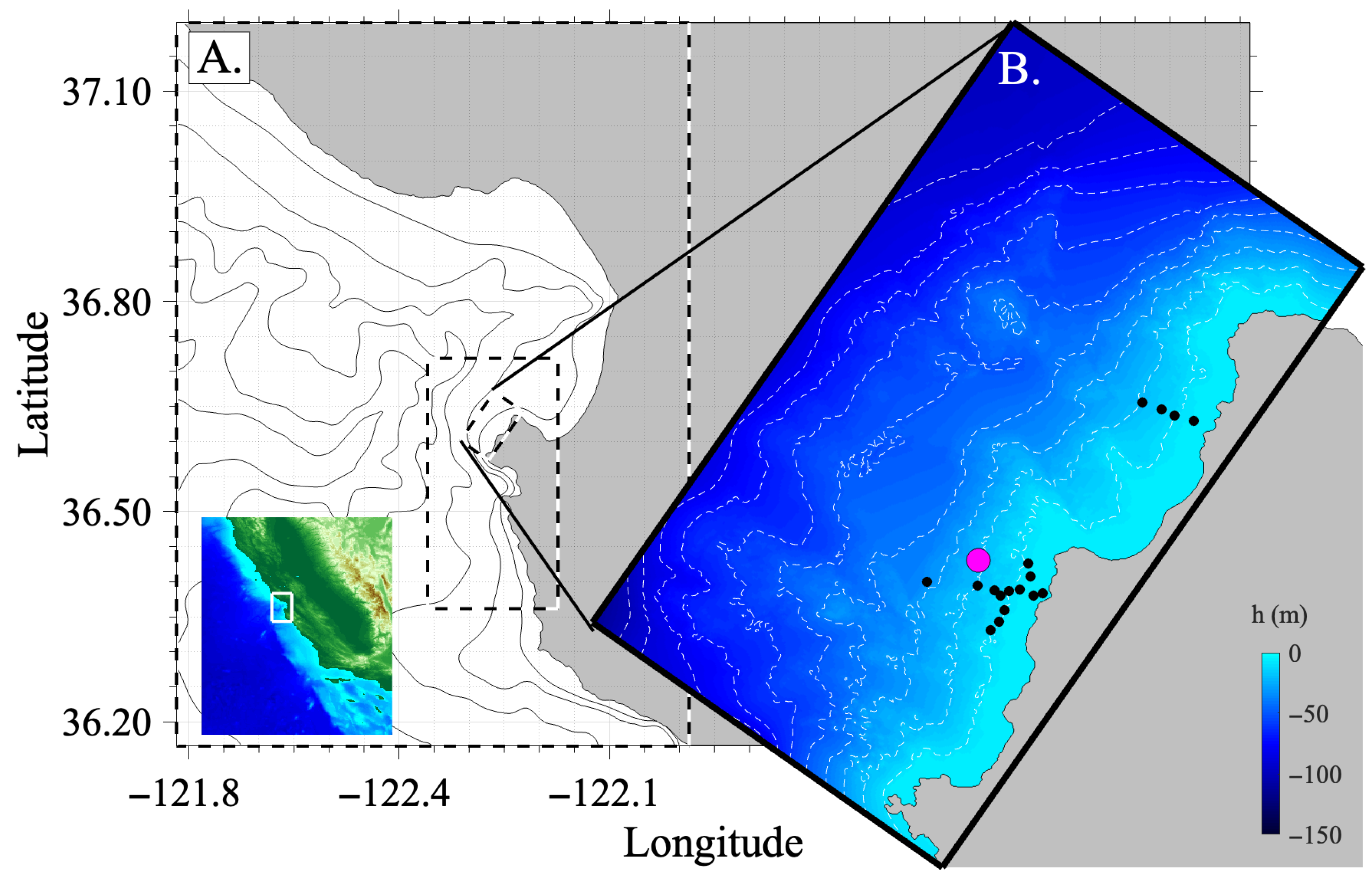
The model domain covers the Monterey Bay and Peninsula (Figure 1) in central California, on the western coast of North America. The Monterey Peninsula extends ≈ 10 km beyond the southern coastline of Monterey Bay (Figure 1). The peninsula has a rocky shore and seabed consisting of quasi-random mounds, platforms, and outcropping features that extend to ≈90 m depth [15,56]. The lowest level of model nesting (parent grid, PG) is 80 × 112 km covering ≈9000 km² with a horizontal grid spacing of 500 m (Figure 1A). The PG includes the Monterey Canyon, which reaches a maximum depth of 2840 m. Subsequently, two levels of one-way model nesting follow. The first child grid (CG1) covers ≈780 km² (20.2 × 38.7 km) with 100 m horizontal resolution, designed to cover the entire Monterey Peninsula. The second nested child grid (CG2) covers an area of 52 km² (9.5 × 5.5 km) and has a horizontal spacing of 20 m (Figure 1B). CG2 is nested within CG1 and covers the location of a nearshore field program that studies rocky shores [21]. The CG2 high-resolution data resolves near-shoreline features, including submerged channels, km-scale embayments, and headlands. The bathymetry used for all three grids was derived from Digital Elevation Models in the NOAA tsunami inundation product [57], with 10 m resolution. A minimum depth of 5 m was set for all SWAN models, with the boundary extended to the shoreline, where it is treated as a closed boundary.

The PG parent grid receives hourly spatially varying boundary conditions (5 km resolution) along the open ocean boundaries (west and south) from the Coastal Data Information Monitoring and Prediction (MOP) system [58]. The MOP system is a high-resolution (100 m × 100 m), non-stationary, linear spectral refraction wave model that combines deep-water buoy observations with a numerical wave-propagation model to predict nearshore waves [58]. MOP covers a range of wave frequencies 0.04 to 1 Hz with a frequency resolution of 0.01 Hz and a directional resolution of 5 degrees. The same frequency and direction ranges are simulated in the SWAN models, but with 50 frequencies and frequency-dependent variable resolution $\mathsf{\Delta }f=0.0185f$. The vector wind is extracted from a three-dimensional Coupled Ocean Atmosphere Mesoscale Prediction System (COAMPS) [59,60,61] with 4 km horizontal resolution, output every 3 h, and used as surface forcing. The formulation for wind-wave generation $S_{in}$ is based on both linear [62] and exponential [63] growth mechanisms. SWAN default coefficients are used for both expressions [55].

2.2.1. Dissipation by Bottom Friction

The wave energy dissipation factor $f_e$, is a key component in wave bottom friction dissipation Equation (2), and similarly the SWAN dissipation term $S_{D_f}$ Equation (4). The dissipation factor is parameterized to be a function of two length scales: the wave excursion distance $A_b$, and the bottom roughness scale $k_N$. The wave excursion is defined as $A_b=U_b/\omega$, where $\omega$ denotes the angular wave frequency ($\omega =2\pi f$), and $U_b=\sqrt{2}{U}_{rms}$. $U_{rms}$ is derived from the frequency spectrum through linear wave theory,

$$U_{\mathrm{rms}}={\left[{\int }_{f_1}^{f_2}{\displaystyle \frac{{\omega }^2}{{sinh}^2\left(kh\right)}}{S}_{\eta }\left(f\right)df\right]}^{1/2}.$$

(6)

The frequency limits $f_1=0.05$ and $f_2=0.2$, are chosen to match the spectral bands in processing observations [21] and isolate the bulk of the wave energy at this location (See Section 3.2).

The ratio, $A_b/k_N$, forms a non-dimensional wave excursion parameter, which is used as the single independent variable to determine $f_e$. The default formulation in SWAN [28], hereafter Ma88, finds $f_e$ through an iterative procedure solving:

$${\displaystyle \frac{1}{4\sqrt{f_e}}}+{log}_{10}\left({\displaystyle \frac{1}{4\sqrt{f_e}}}\right)=m_f+{log}_{10}\left({\displaystyle \frac{A_b}{k_N}}\right)$$

(7)

where $m_f=-0.08$, and a maximum $f_e$ is set in this default formulation at 0.3.

Alternatively, the dependency of $f_e$ on $A_b/k_N$ is often approximated explicitly as (e.g., [36])

$$f_e=exp[a_1{(A_b/k_N)}^{a_2}+a_3],$$

(8)

with $a_1=5.213$, $a_2=-0.194$ and $a_3=-5.977$ [36]. This exponential function was implemented by Rogers et al. [14] to simulate high coral reef $f_e$, termed Ro16, and follows the functional form of Equation (8) until a maximum value of $f_e=50$.

Marques et al. [21] developed a formulation specifically for rocky coasts at the current study site as part of a rocky shore initiative described in Section 2.3 below. The formulation is expressed as a power law relation given by

$$f_e=0.4304{(A_b/k_N)}^{-1.02},$$

(9)

where, in Marques et al. [21], $k_N$ is prescribed as $k_N=4{\sigma }_b$.

2.2.2. Estimation of Variable $k_N$

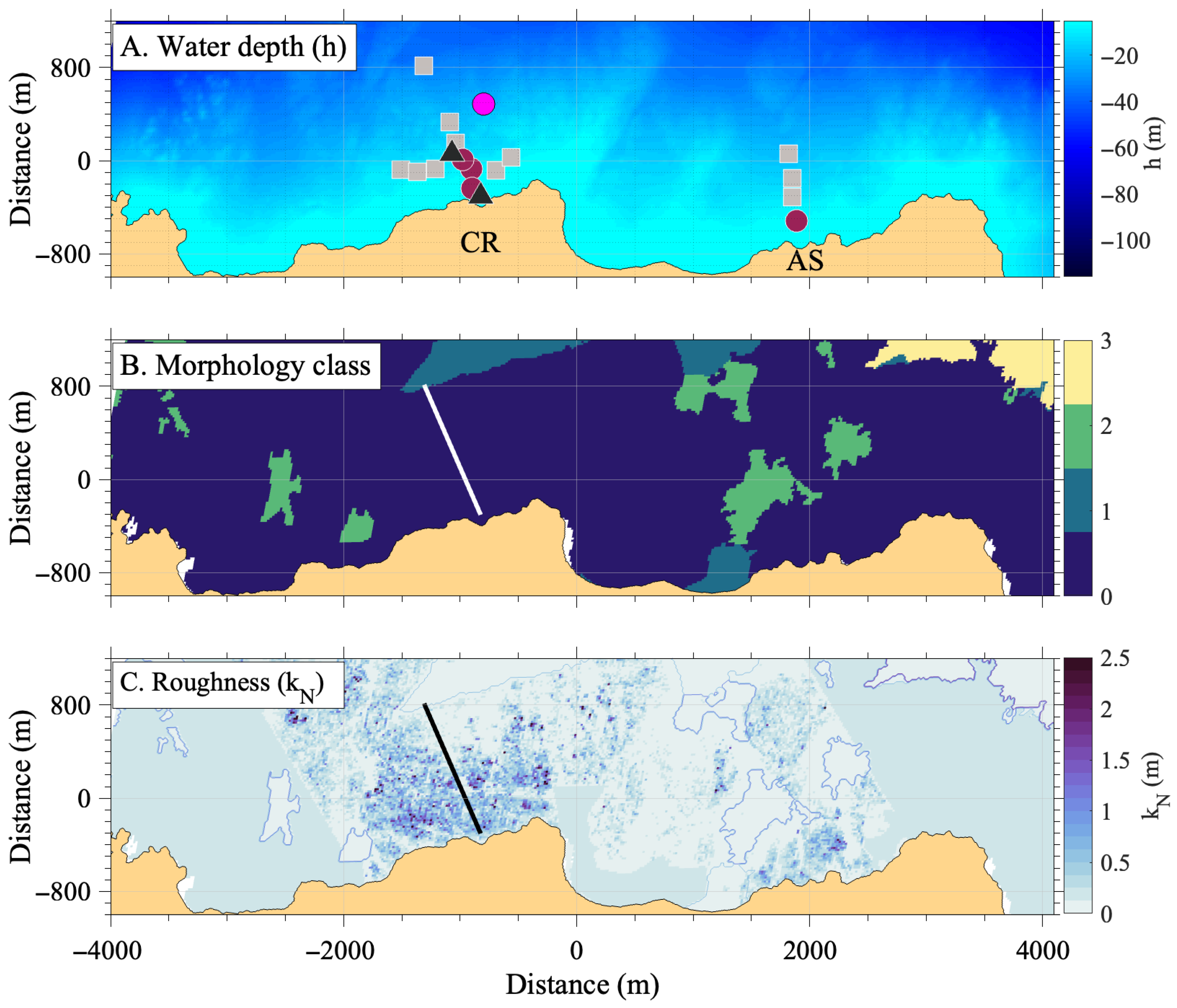
Several simulations with spatially-constant $k_N$ were conducted. In the base-case Rx22 simulation, $k_N=0.5$ m was used. To estimate spatially-varying roughness, high-resolution multi-beam bathymetry was collected at 2 m horizontal-resolution and combined with historical multibeam datasets from California State University Monterey Bay [64], airborne lidar from the Joint Airborne Lidar Bathymetry Technical Center of Expertise (JALBTCX) [65], and echosounder surveys. The combined 2 m resolution product is described in Marques et al. [21]. Following Rogers et al. [29], unresolved bathymetric features at 20 m resolution are represented by a roughness length $z_0$, which serves as a proxy for $k_N$ through:

$$\langle z_0\rangle =a_1\langle h_b\rangle \left({\displaystyle \frac{\langle h_b\rangle }{{\lambda }_x}}\right)+\langle z_{0,ur}\rangle .$$

(10)

Here $\langle h_b\rangle$ is the root-mean-square (RMS) deviation of the bathymetry about a mean bottom slope calculated over 20 m and ${\lambda }_x$ is the dominant wavelength of bathymetric slope variability [29]. Several values of $a_1$ in Equation (10) were tested in calibration simulations against observations. An $a_1=3.2$ yielded the lowest RMSE, when compared to the 20 locations listed in

Table 1. Instrument type, deployment coordinates, deployment duration, and mean water depth. Instrument types are abbreviated as follows: AQD = Aquadopp (Nortek, Rud, Norway), SpB = Spotter (Sofar, San Francisco, CA, USA) buoy, PS = Solo D pressure sensor (RBR, Ottawa, ON, Canada), and SIG = Signature 1000 (Nortek, Norway). DD denotes deployment duration, and h denotes water depth.

Site Code	Type	Lon (°E)	Lat (°N)	DD (h)	h (m)
China Rock
ISPAR	-	−121.968	36.6086	614	24.7
China Rock
B01	SpB	−121.974	36.6061	679	33.9
B03	SpB	−121.9681	36.6057	823	21.4
B05	SpB	−121.9662	36.6052	823	16.3
B07	PS	−121.9644	36.6053	689	13.0
B08	AQD	−121.9632	36.6053	706	11.8
B10	SIG	−121.9626	36.6050	644	9.9
B11	AQD	−121.9621	36.6050	706	10.1
B12	PS	−121.9617	36.6048	811	7.3
B13	SIG	−121.9615	36.6047	706	5.1
Asilomar
X01	SpB	−121.949	36.6269	823	20.9
X03	SpB	−121.9467	36.6262	823	15.8
X04	SpB	−121.9452	36.6255	823	11.2
X05	SIG	−121.944	36.6253	706	9.6
X06	AQD	−121.943	36.6248	688	8.4
Alongshore array
E01	SpB	−121.9666	36.6005	785	10.5
E02	SpB	−121.9656	36.6015	789	12.2
E03	AQD	−121.9639	36.6045	685	10.0
E05	SpB	−121.964	36.6039	720	8.5
E09	SpB	−121.9629	36.6058	788	10.5
E13	SpB	−121.9622	36.6083	787	10.7

. The term $\langle z_{0,ur}\rangle$ represents unresolved roughness elements with scales smaller than the available 2 m resolution and was assumed negligible ($\langle z_{0,ur}\rangle =0$).

Because the CG2 model domain extends beyond the region of available 2 m data, a USGS geologic map of bottom morphology classifications [66] is used (Figure 2B). The classification provides a map of substrate polygons, in which a representative $z_0$ for each type was chosen and then extrapolated to cover the remainder of the CG2 domain (Figure 2C). Although both simpler relations (i.e., $k_N=4\langle h_b\rangle$) and more complicated expressions (e.g., [29,31]) can provide spatially varying $z_0$, a formulation of intermediate complexity is adopted here. Equation (10) is used as a compromise between model simplicity and the ability to represent spatial variability in roughness, with its implications for model–data agreement evaluated in Section 4.1.

2.3. Field Site and Observations

The Rocky Shores Experiments and Simulations (ROXSI) field program (15 June to 20 July 2022) deployed an array of more than 70 instruments (ADCPs, pressure sensors, and buoys) across the nearshore of the Monterey Peninsula [21]. Field collections also included high horizontal resolution bathymetry and drone LiDAR measurements of surface elevation and wave spectra [67]. To evaluate the numerical model in this study, a subset of 20 instruments was selected (Figure 2A, Table 1), with depths ranging from 5 to 34 m. These 20 instruments form two cross-shore arrays at China Rock (CR) and Asilomar (AS), with an additional alongshore array of measurements on the 10 m isobath at CR. Both locations are rough rocky shorelines with minimal sea-swell wave energy reflection [20]. An Inner Shelf Spar (ISPAR) buoy deployed at 24.7 m depth collected meteorological data and includes a GPS-Based inertial motion unit and 3D sonic anemometers [68,69]. Wave-resolving measurements from ADCPs, pressure sensor, and wave buoys provided hourly wave statistics as described in [21,70]. Briefly, hourly spectra were computed with a frequency resolution of ≈(1/120) Hz and 118 degrees of freedom, comparable to standard estimates of wave statistics in other studies (e.g., [71]).

2.4. Wave Parameters and Analysis

Bulk wave statistics were calculated using the SWAN directional spectrum as follows: The significant wave height is related to the variance of the sea surface as

$$H_s=4.0{\left[{\int }_{f_1}^{f_2}{S}_{\eta }\left(f\right)df\right]}^{1/2}.$$

(11)

The mean wave period was calculated as $T_m=m_0/m_1$, where $m_0$ and $m_1$ are the zeroth and first moments of the wave energy spectrum, respectively. The mean wave direction was calculated though directional moments, $a_n$ and $b_n$ defined following [72]:

$$\begin{array}{c}\hfill a_n\left(f\right)={\int }_{-\pi }^{\pi }cos\left(n\theta \right)D(\theta ,f)d\theta \\ \hfill b_n\left(f\right)={\int }_{-\pi }^{\pi }sin\left(n\theta \right)D(\theta ,f)d\theta \end{array}$$

(12)

where the first and second order, $n=(1, 2)$, are estimated from the model. The energy-weighted directional moments are defined as

$$\begin{array}{c}\hfill \overline{a_n}={\displaystyle \frac{{\int }_{f1}^{f_2}{a}_n\left(f\right)S_{\eta }\left(f\right)df}{{\int }_{f1}^{f_2}{S}_{\eta }\left(f\right)df}}\\ \hfill \overline{b_n}={\displaystyle \frac{{\int }_{f1}^{f_2}{b}_n\left(f\right)S_{\eta }\left(f\right)df}{{\int }_{f1}^{f_2}{S}_{\eta }\left(f\right)df}}\end{array}$$

(13)

Then, the mean wave direction is defined as

$${\theta }_m={\displaystyle \frac{1}{2}}{tan}^{-1}\left({\displaystyle \frac{{\overline{b}}_2}{{\overline{a}}_2}}\right)$$

(14)

and the directional spread ${\sigma }_{\theta }$ as

$$\overline{{\sigma }_{\theta }}={\displaystyle \frac{1-\overline{a_2}cos\left(2{\overline{\theta }}_m\right)-{\overline{b}}_{2}sin\left(2\overline{{\theta }_2}\right)}{2}}$$

(15)

The model’s performance is evaluated using 3 skill metrics: mean bias, root mean square error, and Wilmott skill [73,74]. These are defined as

$$\begin{array}{cc}\hfill MB& =\langle m\rangle -\langle o\rangle \hfill \\ \hfill RMSE& ={\langle {(m-o)}^2\rangle }^{1/2}\hfill \\ \hfill WSS& =1-{\displaystyle \frac{RMS{E}^2}{\langle {\left(|m-\langle o\rangle |+|o-\langle o\rangle |\right)}^2\rangle }}.\hfill \end{array}$$

(16)

Here, m and o are time series of modeled and observed variables, respectively, and $\langle ·\rangle$ denotes a time-mean. The Willmott skill score is such that $WSS$ = 1 (0) indicates complete agreement (disagreement) between observed and modeled quantities.

3. Results

3.1. Wind and Wave Conditions

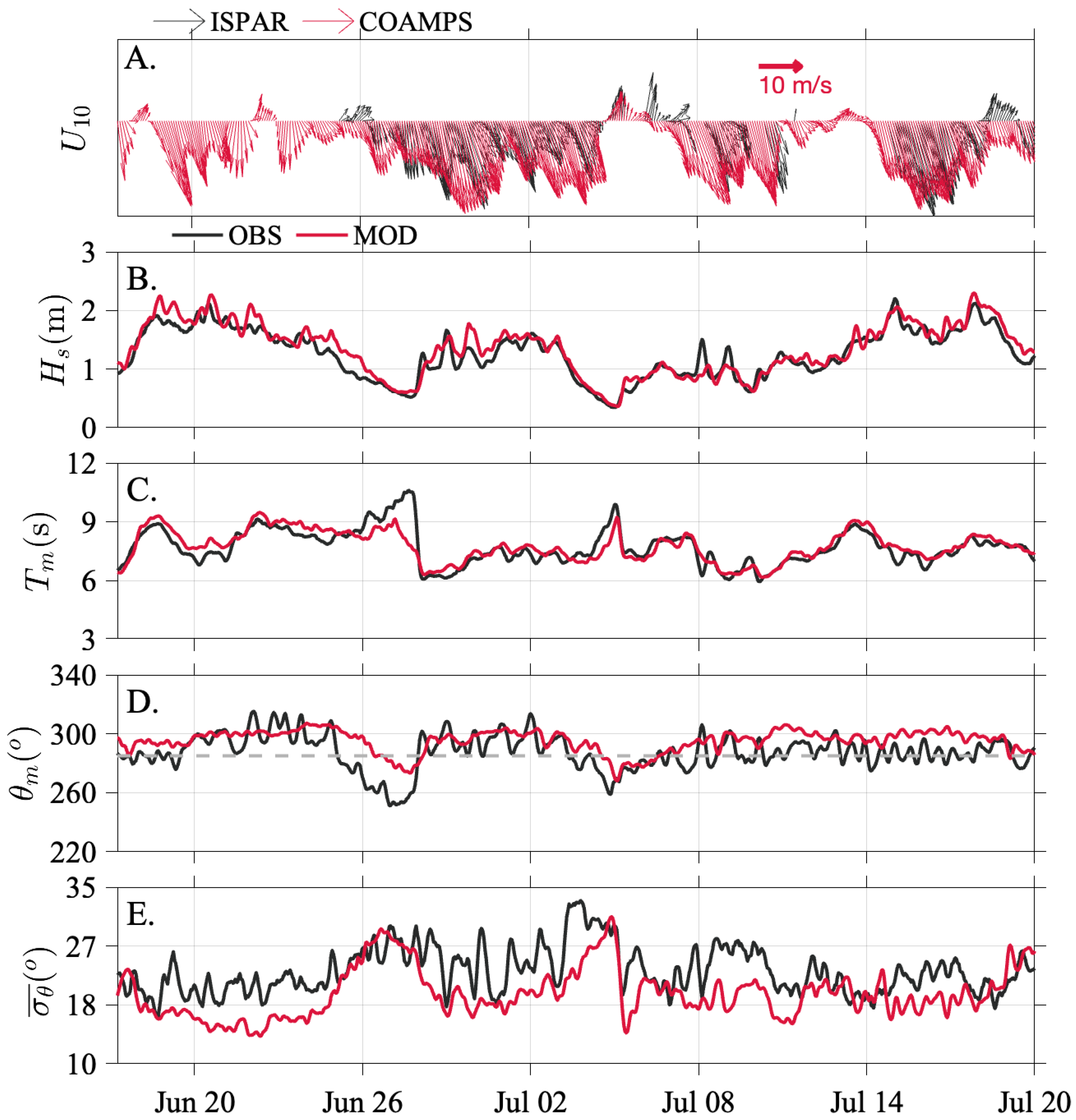
Consistent with the summer regional climatology (e.g., [75]), the wind vectors 10 m above sea level were predominantly from the northwest, interrupted by reversal events (from the southeast) during the study period (Figure 3A). The wind forcing from COAMPS shows good agreement in both direction and magnitude with offshore measurements from the ISPAR buoy (see location, Figure 1A). The northwest wind periods were longer, lasting 3 to 5 days, compared with the southeast wind periods, which lasted 1 to 3 days. The wind speed was also higher during the northwest wind periods, reaching 12 m/s, while during the southeast winds it was 3 to 5 m/s. During NW wind periods, the significant wave height $H_s$ observed at B03 (water depth of 22 m) was higher than during the SE wind periods, 1–2.4 m versus 0.5 to 1.5 m (Figure 3B). During NW wind periods, the mean wave direction ${\theta }_m$ is mostly centered around the shore normal direction (285°), gray dotted line, (Figure 3D), becoming more aligned with the wind during these high wind events (≈285°). Bulk wave directional spread ${\sigma }_{\theta }$ is fairly constant at 24°, throughout the study (Figure 3E). During periods of weak southerly wind, south-ocean swell wave characteristics such as lower energy, longer period, and southerly direction tend to dominate the observed signals at B03 ($H_s<1$ m, $T_m$ up to 9 s, and ${\theta }_m \approx 230$°). The ${\sigma }_{\theta }$ tends to be higher during these periods with values > 30° due to a wave spectrum with comparable wave energy arriving from distinct directions, NW and SE.

3.2. Model Validation

The bulk wave characteristics simulated in Rx22 are evaluated against observations at the B03 mooring ($h=21.4\mathrm{m}$), situated approximately $700\mathrm{m}$ offshore. Overall, the model shows strong agreement with measurements, with Willmott skill scores of 0.96 for $H_s$ and 0.97 for $T_m$ (Figure 3B,C). The wave direction (${\theta }_m$) also aligns well with observations during the first two weeks of deployment. However, the largest model-data discrepancy (25°) occurs on 26 June during a wind relaxation event when $H_s$ is small. At this time, observed waves arrive obliquely from the southwest, while the model predicts a more shore-normal direction. In the latter half of the study, the model consistently offsets ${\theta }_m$ by 15°, predicting a more northerly wave direction than observed.

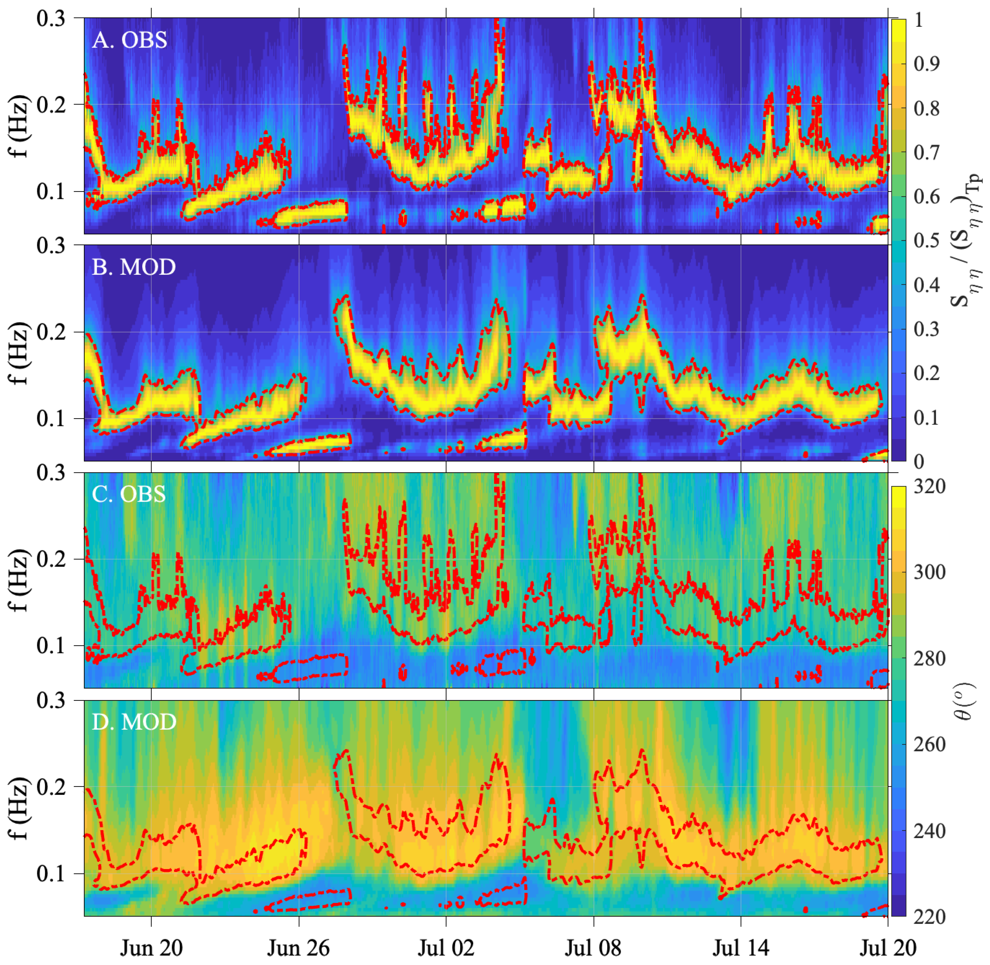
In addition to comparing bulk spectral characteristics at B03, we also analyzed the hourly frequency-dependent wave energy $S_{\eta }$ and the wave directional spectrum $D\left(f\right)$ at this buoy (Figure 4). To facilitate a frequency-dependent comparison, $S_{\eta }$ is normalized by the hourly energy at the peak frequency. A dashed red contour in Figure 4 highlights frequencies that contain ≥50% of the total energy at the hourly peak frequency. The energy distribution between 0.05 and 0.2 Hz contains, on average 70–80% of the hourly wave energy and is very similar in both the observations and the model (Figure 4A,B). In both model and observations, the locally generated sea and swell (0.08 to 0.2 Hz) predominantly propagates from the northwest (280° to 320°). The presence of remote swell (0.06–0.08 Hz) is also evident in both the model and observations. The remote swell is noticeable throughout most of the study period but only affects bulk statistics when wind speeds are low (Figure 3A). Less energetic observed high-frequency local seas (0.2 Hz $<S_{\eta }<$ 0.3 Hz) appear to have more pronounced variability that is not as well reproduced. At high frequencies (>0.2 Hz), the observed wave direction exhibits greater variability, ranging from 260° to 320°, whereas the model predicts a narrower range of 290° to 320°, possibly due to the strong Monterey Bay sea-breezes that are not well represented here. Although at 4 km resolution, the atmospheric model used here is higher than previous studies at this location [59,76], alternate wind-input source term implementations could be compared (e.g., [76,77]). A dedicated sensitivity analysis is beyond the scope of the present study.

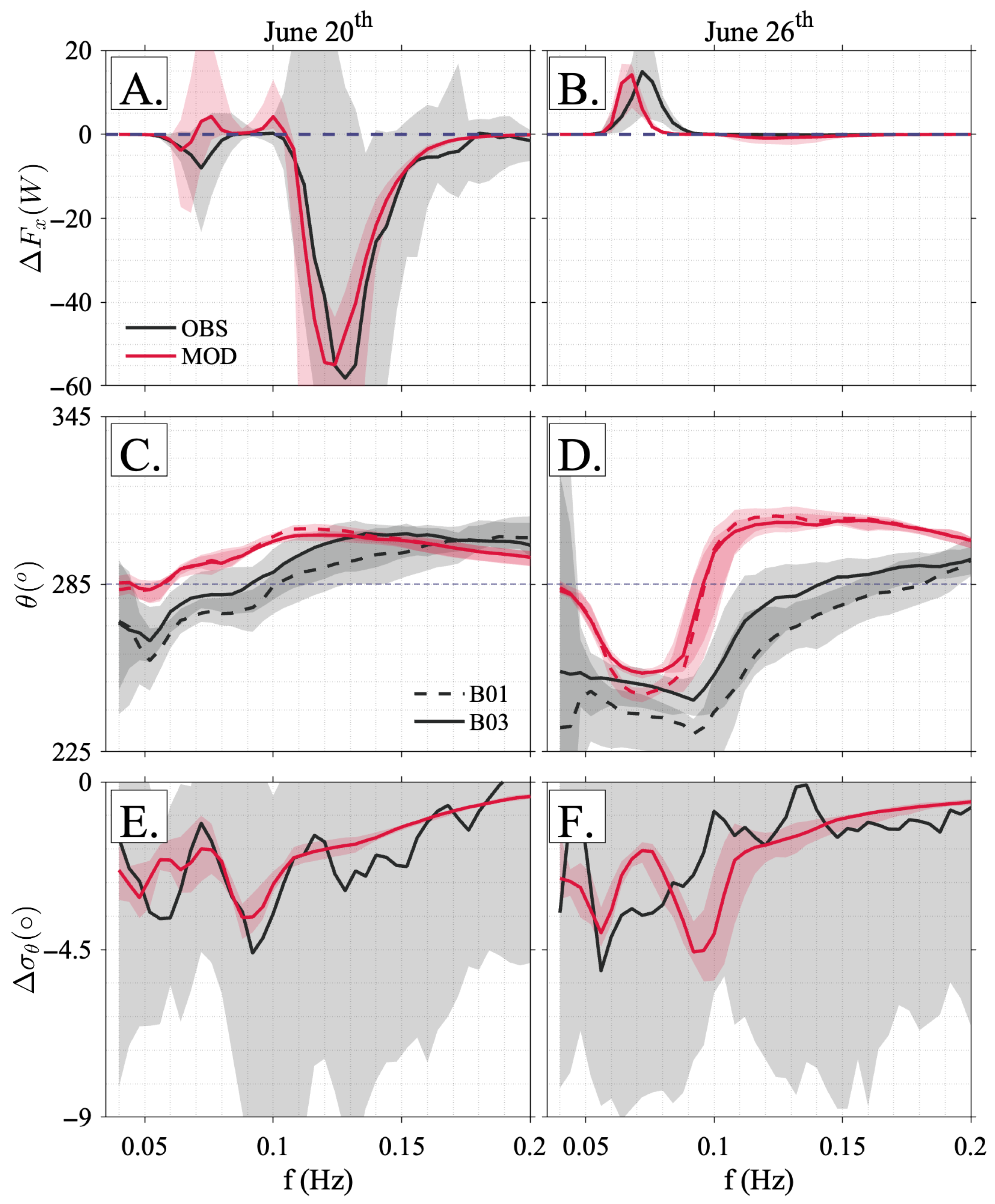
We assessed SWAN’s ability to simulate the observed spectral transformation across the nearshore by computing the difference $\mathsf{\Delta }$ in wave parameters between a pair of buoys at all modeled frequencies. We examine wave energy flux, wave direction, and directional spread between two wave buoys, B01 and B03 (see map, Figure 1), under different conditions: one day dominated by locally generated sea-swell (20 June) and another by remote swell (26 June) (Figure 5). The difference in daily-median energy flux difference ${\langle \mathsf{\Delta }{F}_x\rangle }_{p50}$ exhibits distinctly different behavior between the two days, which is reasonably well captured by the model. On 20 June, ${\langle \mathsf{\Delta }{F}_x\rangle }_{p50}$ decreases, with a pronounced negative peak at 0.125 Hz, indicating energy flux convergence between buoys (Figure 5A). In contrast, under remote swell-dominated conditions on 26 June, ${\langle \mathsf{\Delta }{F}_x\rangle }_{p50}$ increases at frequencies between 0.05 and 0.1 Hz, showing wave energy divergence (Figure 5B). For both conditions, SWAN provides a good estimate of the magnitude of ${\langle \mathsf{\Delta }{F}_x\rangle }_{p50}$ and the frequencies at which convergence and divergence occur.

For the local sea-swell dominated day, SWAN well estimates the wave direction across all frequencies (Figure 5C). During this day, wave directions at all frequencies are mostly aligned with the wind and fairly shore-normal in agreement with regional wave characteristics [75,78]. During the day dominated by remote swell, swell directions are more southerly in both the model and observations (Figure 5D), distinct from the lower energy local waves (>0.1 Hz). Between buoys, observed waves clearly refract towards shore normal (black solid to black dashed lines in Figure 5C,D). This is especially clear on 26 June, where 0.12 Hz refracts by ≈10° between B01 and B03. Refraction is also evident in the model results, particularly on 26 June, though the signal is not as strong as observed. At all frequencies, both observed and modeled, the difference in wave directional spread between B01 and B03 ${\langle \mathsf{\Delta }{\sigma }_{\theta }\rangle }_{p50}$ is negative, indicating a decrease as waves propagate shoreward. This effect is consistent with wave refraction and is especially strong in the low-frequency swell band ≈ 0.05 Hz.

3.3. SWAN Modeled Energy Source Terms Across the Nearshore

The predominant controls on modeled wave energy are identified by comparing individual source terms in the SWAN action balance equation (Equation (5)). A transect of Rx22-simulated hourly terms is extracted at the 20-m grid (CG2) extending from the shoreline to 1500 m offshore following locations of the China Rock observational array (Figure 1).

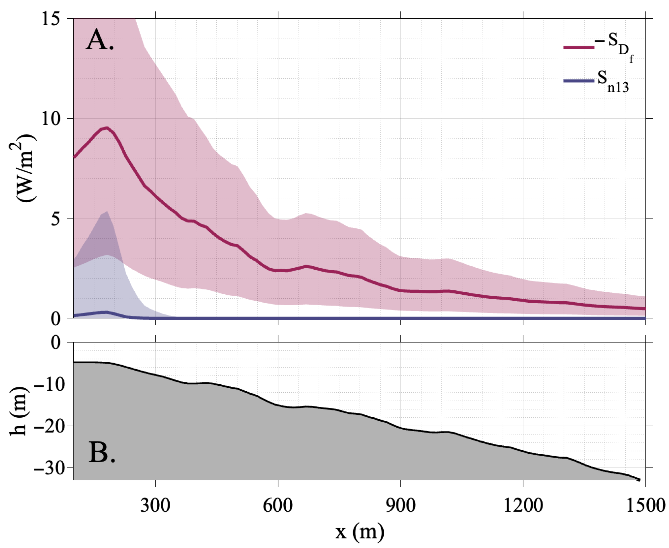
Across this nearshore transect, bottom friction dissipation is the dominant term in the energy balance equation, leading to a loss of wave energy. The predominance of $S_{D_f}$ increases in shallow water, reaching a maximum in the time-median value of $8\mathrm{W}/{\mathrm{m}}^2$ in $5\mathrm{m}$ depth (red line in Figure 6A). In addition, the temporal variability of $S_{D_f}$ is also orders of magnitude larger than the other terms in Equation (5). The only other source term that is significant relative to bottom friction dissipation is the non-dissipative three-wave interaction term $S_{n13}$ that represents a transfer of energy across wave frequencies and results in no net change in frequency-integrated wave energy metrics such as $H_s$. $S_{n13}$ increases in importance at ≈10 m depth and reaches a maximum median value of ≈2 $\mathrm{W}/{\mathrm{m}}^2$ with $10\mathrm{W}/{\mathrm{m}}^2$ of variability at 5 m depth (Figure 6A). High $S_{n13}$ instances occur during the highest energy wave conditions ($H_s>2$ m). We note that the 10 m depth is 350 m from the shore and far from the offshore boundary of the model domain, where a mostly linear wave spectrum evolution can be anticipated. The other source terms in (5) have relatively small median and temporal variability (<$\mathrm{O}\left({10}^{-1}\right)\mathrm{W}/{\mathrm{m}}^2$) relative to $S_{D_f}$ and $S_{n13}$. The non-dissipative $S_{n14}$ has an $\mathrm{O}\left({10}^{-2}\right)\mathrm{W}/{\mathrm{m}}^2$ range of variability, and wave energy growth by the wind $S_{in}$, dissipation due to white-capping $S_{ds,w}$, and wave breaking $S_{D_b}$ are all $\mathrm{O}\left({10}^{-3}\right)\mathrm{W}/{\mathrm{m}}^2$ or smaller. Thus, bottom friction is the dominant process that requires accurate simulation across this water depth range of rocky nearshore environments.

3.4. Comparison of Base Case Simulation to Default SWAN

To evaluate the impact of wave friction formulations on model performance, we compare the base-case Rx22 model, which uses the Marques et al. [21] power law relation for $f_e$, to a simulation with identical grids, $k_N$, boundary and surface forcing, but using the default SWAN $f_e$ parameterization from Madsen et al. [28] (Ma88). To achieve a single value for mean bias (MB), root mean square error (RMSE), and Willmott Skill score (WSS), bulk wave parameters from each simulation are compared to observations across all instrument locations (

Table 2. Assessment of model bulk wave statistics compared to observations with mean bias MB, root mean square error RMSE, and Willmott Skill score WSS. Units for MB and RMSE are $H_s$ (m), $T_m$ (s), ${\theta }_m$ (^o), ${\sigma }_{\theta }$ (^o). Bulk statistics are calculated across the frequency range of 0.05 to 0.2 Hz.

Case	Metric	${\mathit{H}}_{\mathit{s}}$	${\mathit{T}}_{\mathit{m}}$	${\mathit{\theta }}_{\mathit{m}}$	${\mathit{\sigma }}_{\mathit{\theta }}$
Rx22 $k_N=0.5$	RMSE	0.17	0.51	9.11	4.43
	MB	0.05	0.08	−3.36	−1.42
	WSS	0.95	0.91	0.59	0.53
Ma88 $k_N=0.5$	RMSE	0.23	0.53	8.87	4.44
	MB	0.16	0.21	−3.00	−1.26
	WSS	0.91	0.91	0.62	0.53
Ro16 $k_N=0.5$	RMSE	0.17	0.55	9.69	4.39
	MB	0.03	0.01	−3.82	−2.38
	WSS	0.94	0.90	0.57	0.59
Ro16 $k_N=1.0$	RMSE	0.22	0.68	9.72	4.44
	MB	−0.14	0.23	−5.08	−1.99
	WSS	0.90	0.84	0.56	0.54
Rx22var	RMSE	0.18	0.51	8.97	4.39
	MB	0.06	0.15	−3.23	−1.70
	WSS	0.94	0.91	0.61	0.56

). The bulk skill metrics for mean wave period $T_m$ and the directional parameters ${\theta }_m$ and ${\sigma }_{\theta }$ are very similar between Rx22 and Ma88 simulations with $k_N=0.5$ m. Although the bulk WSS values for significant wave height $H_s$ are similarly high between the simulations, MB and RMSE are modestly improved in Rx22 relative to Ma88 (Table 2). A discussion of model-data evaluation from additional simulations (Ro16 and Rx22^var) follows in Section 4.1.

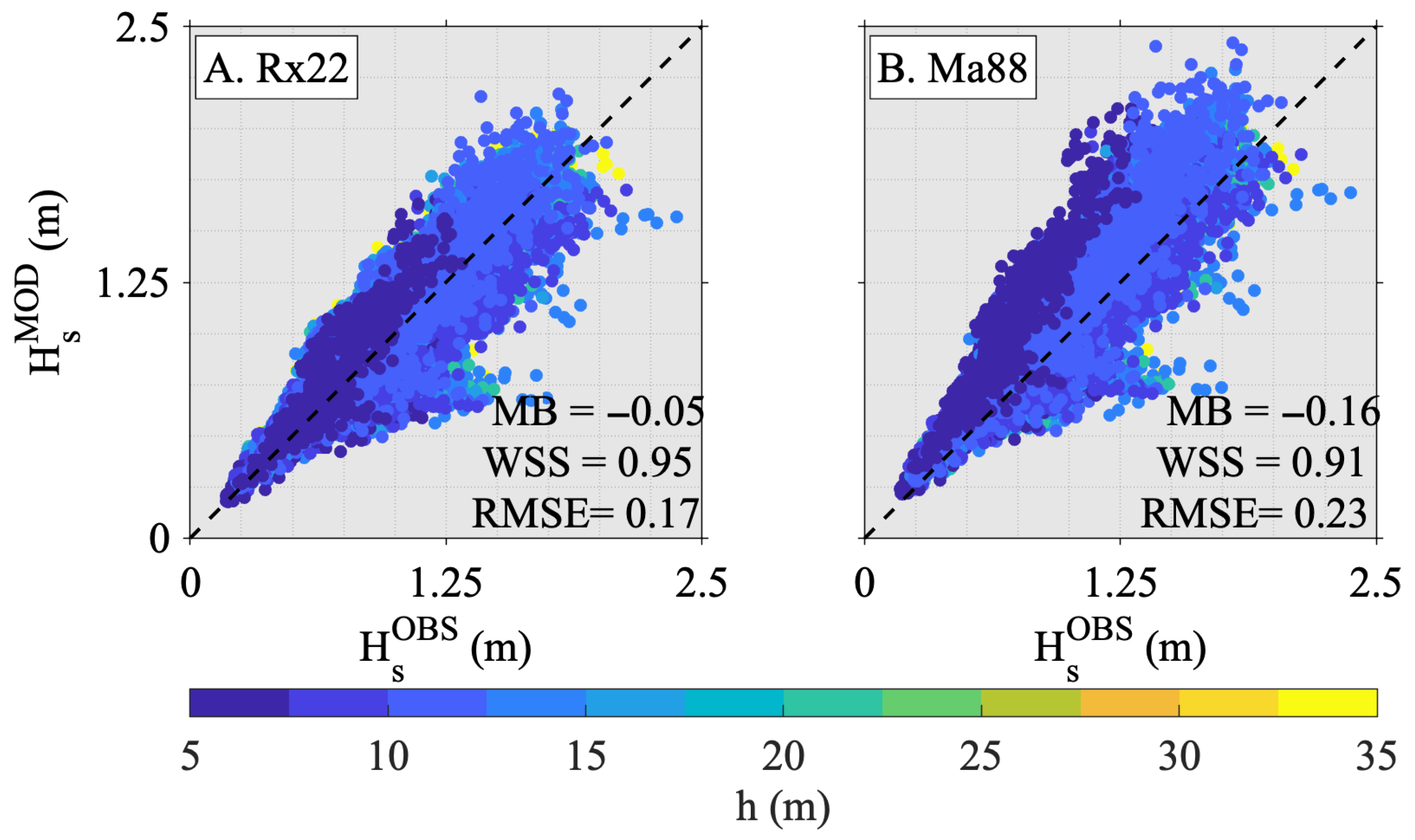
Similarity in bulk WSS between simulations is also evident from overall proximity to a one-to-one line between model results versus observations (Figure 7). Differences between the model and observations are clearer at individual water depths. For example, comparisons of $H_s$ in $h=5$ m in Rx22 (dark blue, Figure 7A) appear more closely aligned with the one-to-one line relative to Ma88 (dark blue, Figure 7B). In particular, in shallow waters, the Ma88 model overestimates $H_s$ relative to observations. Given that the only difference between Rx22 and Ma88 lies in the formulation of $f_e$, this overestimation in shallow water is attributed to reduced bottom dissipation in the Ma88 parameterization relative to Rx22. This process appears to be increasingly important at shallower depths. Therefore, while bulk skill metrics (e.g., Table 2) show strong overall performance with both Rx22 and Ma88 exhibiting similar results, reliance on an overall score may mask important variations in performance in different modeled regions.

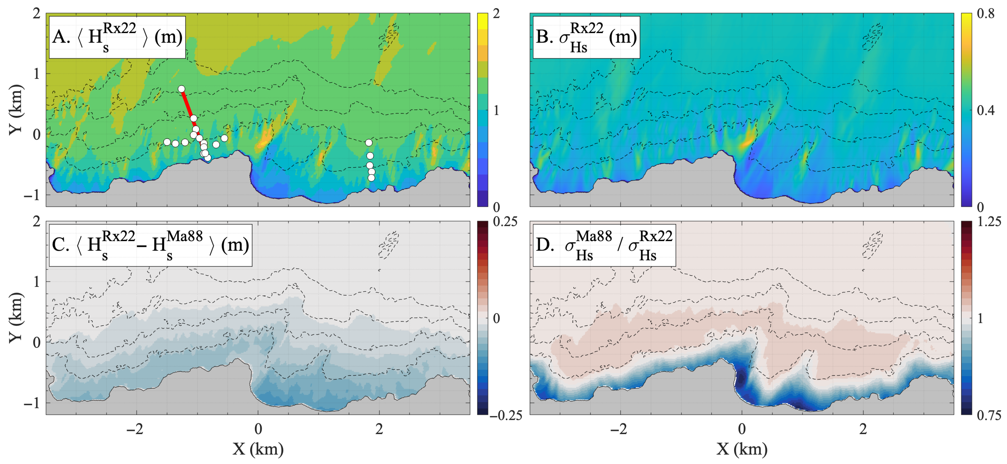
To explore differences between the simulations beyond individual measurement locations, spatial maps of time-average and standard deviation of $H_s$ are compared (Figure 8). Time-average $\langle H_s\rangle$ in Rx22 generally decreases with decreasing depth (Figure 8A). Bathymetric features such as headlands, embayments, and channels alter modeled $\langle H_s\rangle$, consistent with nearshore wave focusing and refraction producing localized variability in both the mean and standard deviation fields (Figure 8B). The difference $\mathsf{\Delta }{\mathrm{H}}_{\mathrm{s}}=\langle {\mathrm{H}}_{\mathrm{s}}^{\mathrm{Rx}22}-{\mathrm{H}}_{\mathrm{s}}^{\mathrm{Ma}88}\rangle$ highlights the region where the default SWAN Ma88 over-predicts $H_s$. This is primarily a function of water depth, beginning around the 25 m isobath and increasing towards shore. Differences range from 0.10 to 0.20 m, and are largest in the shallow portions of embayed regions (Figure 8C). In addition to a reduced mean wave height in Ma88, the variability of $H_s$, expressed as the ratio of standard deviations between Ma88 and Rx22 (${\sigma }_{H_s}^{\mathrm{Ma}88}/{\sigma }_{H_s}^{\mathrm{Rx}22}$), is reduced by approximately $25\%$ at water depths shallower than 10 m (Figure 8D).

4. Discussion

4.1. Inter-Comparison of Models with Different $f_e$ Formulations with Water Depth

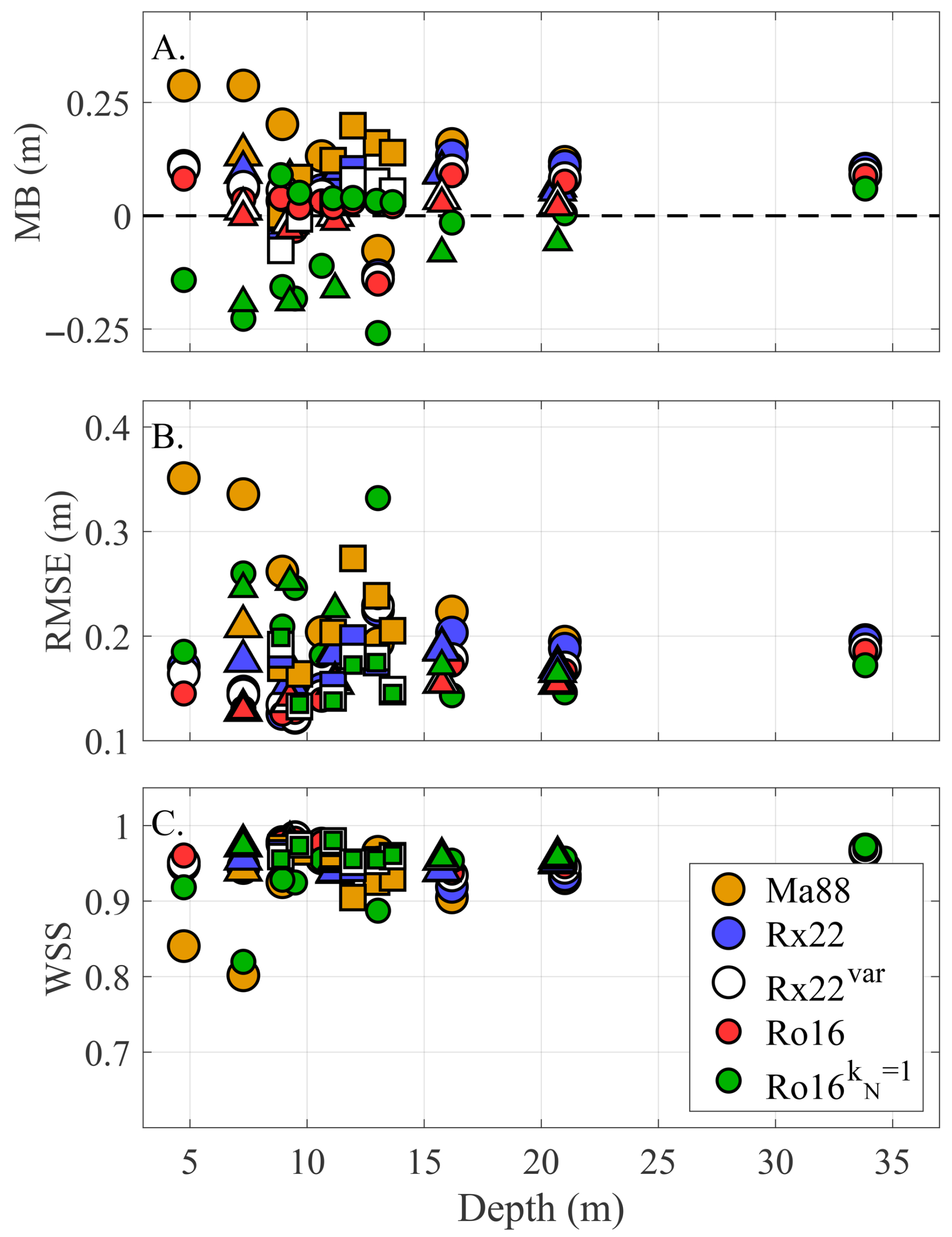
As bottom dissipation becomes increasingly important in shallow water, skill metrics are subsequently examined at individual instrument locations as a function of water depth (Figure 9). In addition to the base-case Rx22 and SWAN default Ma88 simulations, three additional simulations were run for comparison: a simulation with additional complexity in the form of a spatially-varying $k_N$, Rx22^var; a simulation with the Rogers et al. [14] exponential $f_e$ function with the same $k_N$ as Rx22, Ro16; and a simulation with spatially-uniform larger $k_N=1$, Ro16^k_N=1. All three $H_s$ skill metrics are very similar at the deepest measurement location (B01, $h=33.4$ m) for all simulations. In addition, the skill metrics are similar across all inner shelf water depths for Rx22, Rx22^var, and Ro16 simulations. The mean bias falls between $\pm 0.15$ m at all observation locations, except for the Ma88, where the mean bias increases to 0.29 m at the shallowest site (Figure 9A). Mean bias for Ro16^k_N=1 becomes −0.26 m as the larger $k_N$ results in dissipation that is too strong relative to observations. Similarly, the Rx22, Rx22^var, and Ro16 simulations have small root mean square error (<0.24 m) at all observation locations, while Ma88 RMSE increases in shallow water (Figure 9B).

Wilmott Skill scores for $H_s$ in all simulations are above 0.9 between 33.4 and 7.5 m water depth. In contrast, WSS scores decrease in shallow water for Ma88, dropping to ≈0.8 in 7.5 and 5 m water depth. Taken together, the three simulations, Rx22, Rx22^var, and Ro16, remain relatively accurate compared to observations across the inner shelf region, whereas the default SWAN simulation Ma88 accumulates error with decreasing depth. The primary difference is that the wave friction $f_e$ parameterization in Rx22, Rx22^var, and Ro16 include higher values than the default SWAN (0.3), and that these values are necessary to simulate waves across the rough substrate of rocky inner shelf water depths, mirroring SWAN simulations over rough coral reef environments [14]. It appears that neither the functional form of $f_e$ nor the additional complexity of a spatially variable roughness $k_N$ consistently results in model improvement.

4.2. The Friction Factor $f_e$ Appropriate for Rocky Shores and Its Relation to $A_b/k_N$

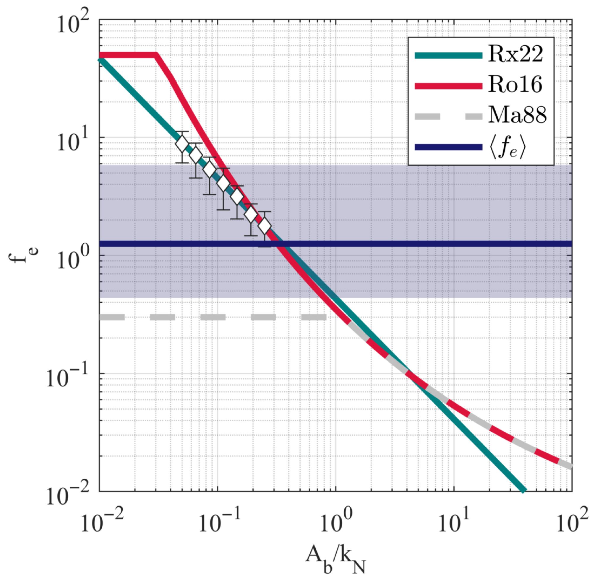
The wave friction factor $f_e$ is commonly reported in nearshore studies over rough seabeds. To contextualize our rocky shore modeling with these studies, we compare Rx22 modeled $f_e$ across the CR transect (34–5 m water depth). The majority of $f_e$ estimates, 80%, fall within the range of 0.43 to 5.38, with 98% of $f_e$ values exceeding the SWAN default of 0.3 (Figure 10). Observationally, in the same study Marques et al. [21] reported average $f_e$ values with a similar range (1.1–5.1). These $f_e$ values also encompass the 1.8 reported by Monismith et al. [13], and are within the 0.5–5 range documented by Lentz et al. [32] over coral reefs.

Given the complexity of wave transformation over rough seabed environments and the potential for non-unique modeling solutions, several aspects are highlighted. First, modeled $f_e$ varies with roughness length $k_N$, even under identical incident wave conditions. This variation can affect model performance, and determining a single representative $k_N$ in a hydrodynamic setting influenced by both waves and mean currents remains a challenge [23,29]. In this study, a spatially constant $k_N=0.5$ produced the best agreement with rocky shore observations, and is of the same order as values reported in studies of coral reefs [6,14,23].

Despite the above consistency, we note several potential discrepancies. First, using the nominal relation of $k_N=4{\sigma }_b$, Marques et al. [21] estimates a mean $k_N$ of approximately 3.2 m near the observation locations. This is a much higher value than the average $k_N=0.5\mathrm{m}$, which yields good model-data agreement. Although $k_N=3.2$ was not tested here, simulations with large $k_N=1$ (Figure 9) already produce wave energy dissipation that is much too strong relative to observations. The difference may be partly explained by the rocky portions of the shore targeted by the observational program, whereas the USGS granitic substrate polygon covers only about 67% of the model domain. The remaining softer bottom types, such as sediment-covered areas and nearshore deposits, likely contribute to a lower average $k_N$ used to achieve favorable model results.

Second, despite the observed $f_e$ and ${\sigma }_b$ spatial co-variation at this location [21], the SWAN simulation with spatially-variable $k_N$, Rx22^var did not increase model-data agreement relative to the base case Rx22. The discrepancy potentially arises from the methodology to estimate roughness metrics from high-resolution bathymetry that depends on the analysis window size [37]. Increasing the analysis window progressively transfers larger-scale bathymetric variability to inferred roughness and thus alters derived $k_N$ (e.g., Equation (10)). As high-resolution bathymetry (Figure 2C) was also not available everywhere in the model domain, sensitivities to estimating $k_N$ from bathymetry were not tested here. The skill metrics between both models that utilize empirically derived relationships between $f_e$ and $A_b/k_N$, the power law relation (Rx22, Equation (9)), and the exponential function (Ro16, Equation (8)) are nearly equivalent. Within the two orders of magnitude of modeled range $0.1<A_b/k_N<1$, $f_e$ monotonically decreases as a function of $A_b/k_N$ and both line slopes and curvature are similar (Figure 10). Although this suggests either choice of empirical model is appropriate for the rocky shoreline here, we advise caution in conditions where $A_b/k_N$ falls outside the current modeled range, as Ro16 and Rx22 curves can substantially diverge (e.g, $A_b/k_N\ll 0.1$ or $A_b/k_N\gg 10$).

At $A_b/k_N\gg 10$, $f_e$ should tend towards the more familiar bottom friction regime associated with a fixed bed substrate of small roughness elements and a well-defined shear-driven turbulent boundary layer. In modeling these cases, the $f_e$ line of Ro16 (Equation (8)) closely matches the Madsen et al. [28] SWAN default (Equation (7)). When modeling this regime, the Rx22 curve should be adjusted, as it is well calibrated by many previous observations and laboratory experiments c.f., [14], Figure 5. The $A_b/k_N\ll 0.1$ parameter space is much less explored c.f., [21], Figure 10, though coral reef and rocky shoreline wave research is growing in nearshore oceanography (e.g., [13,14,15,21,30,31]). A feature of this regime is the fundamental discrepancy between physical and hydrodynamic roughness. At low values of $A_b/{\sigma }_b<1$, DNS simulations suggest that when drag and inertial forces are separated, $f_e$ increases as a function of $A_b/{\sigma }_b$ [41]. In the regional, wave-averaged SWAN model and for bottom dissipation over 10–10⁴ m spatial scales, this positive relationship between $f_e$ and $A_b/k_N$ is not apparent. As demonstrated by Chung et al. [46], flow responses to roughness are highly nonlinear, especially under high Reynolds numbers or intermittent flow separation, where drag becomes decoupled from topographic metrics. Therefore, the $k_N$ in wave models may not be a direct measure of physical roughness but a hydraulic proxy derived from drag. While relations such as $k_N=4{\sigma }_b$ or Equation (10) provide approximate links between physical and hydraulic roughness, alternative formulations that incorporate higher-order bathymetric statistics, such as slope, skewness, orientation, and the size of the evaluated area (i.e., separation length or window size), may help bridge the gap between geometry and hydraulics in heterogeneous environments [17,37,46].

4.3. Note on Model Performance and Alternate Model Configurations

In this work, all model runs with realistic wind forcing and spatially variable 2D boundary conditions capably simulate the spatial and temporal variability of wave energy incident on the Monterey Peninsula inner shelf (Section 3.2), including the observed frequency-dependent refraction and focusing effects between the outermost buoys (Figure 5). In particular, model results at ≈22 m depth closely follow the observed time-varying wave bimodal energy frequency and directional distributions (Figure 4). During summer, the predominant wave frequencies (≥0.1 $\mathrm{Hz}$) are indicative of local wind swell and arrive from the northwest aligned with the wind [75]. The regional wave climate also includes significant signatures of a lower energy remote low-frequency Pacific Ocean swell (≈0.07 $\mathrm{Hz}$) from the southwest [75].

A key element of the Rx22 setup is the use of a time- and spatially variable 2D wave-directional spectrum from the regional CDIP-MOP model as boundary forcing [58]. The MOP product is constrained by directional buoy observations, enabling accurate representation of both local and remote swell energy and directions across frequency bands. While nonlinear spectral transfers become important in shallow water (Section 3.4, Figure 6), at the offshore boundary, linear regional models such as MOP offer an advantage to force local models in regions where bimodal spectral characteristics are significant [79].

No implementation of shoreline wave reflection was included in the current SWAN simulations. Both China Rock and Asilomar locations are characterized by a rough rocky shoreline with small observed wave reflection coefficients (3–6%) [20]. Therefore, inclusion of shoreline reflection is not likely to improve model–data comparison. However, the same is not likely true for other nearshore regions with rocky platforms and/or steep rocky cliffs that have observed sea-swell reflection coefficients of 15–30% [20]. Although beyond the scope of this current manuscript, subsequent ROXSI field and modeling programs will address these topics.

5. Summary and Conclusions

A realistic simulation of surface gravity waves across the rocky shores of Monterey, CA, was performed using a triply nested SWAN model spanning regional and local scales. Comparison with 20 observational sites demonstrates that the model well reproduces the frequency-directional characteristics of surface waves across the nearshore under a range of conditions: relatively low energy waves dominated by southern swell and high energy local waves aligned with strong north-westerly wind conditions ($H_s\approx$ 2 m and wind speed $>10$ m/s). When including a modified bottom friction parameterization, the model performs well and reproduces bulk wave statistics of $H_s$ and ${\theta }_m$ across several skill metrics, despite a positive model bias ≈ 15°. Spatially variable, two-dimensional directional wave spectra boundary forcing is essential to favorable model-data comparison, as sea and swell frequency bands arrive from distinct directions to Monterey Bay.

The primary source term in the modeled wave energy balance equation is the energy sink from bottom friction dissipation, and its representation is critical to model performance across the inner shelf. Two empirical formulations relating normalized wave excursion to wave friction factor $f_e$ result in good model-data agreement: an observationally-derived power-law relation [21] and an exponential relation previously applied to coral reef environments [14]. Two aspects are crucial in these formulations relative to the default in SWAN. First, friction factors are higher than the SWAN default ($f_e=0.3$) and are needed to model increased bottom friction dissipation over a rocky seabed. Second, both formulations maintain an inverse relationship between $f_e$ and wave excursion $A_b/k_N$ over two orders of magnitude of variability $0.1<A_b/k_N<1$ with a large bottom roughness length scale characteristic of rocky shores.

References

1. Koch, E.W.; Barbier, E.B.; Silliman, B.R.; Reed, D.J.; Perillo, G.M.; Hacker, S.D.; Granek, E.F.; Primavera, J.H.; Muthiga, N.; Polasky, S.; et al. Non-linearity in ecosystem services: Temporal and spatial variability in coastal protection. Front. Ecol. Environ. 2009, 7, 29–37. [Google Scholar] [CrossRef] [Scilit]
2. Thomas, T.J.; Dwarakish, G. Numerical Wave Modelling—A Review. Aquat. Procedia 2015, 4, 443–448. [Google Scholar] [CrossRef] [Scilit]
3. Lavidas, G.; Venugopal, V. Application of numerical wave models at European coastlines: A review. Renew. Sustain. Energy Rev. 2018, 92, 489–500. [Google Scholar] [CrossRef] [Scilit]
4. Xu, S.; Ma, M.; Yin, K.; Tang, S. Risk evaluation system of navigation security based on coupled wind and wave model: A case of study of Qiongzhou strait. IET Intell. Transp. Syst. 2020, 14, 1311–1318. [Google Scholar] [CrossRef] [Scilit]
5. Baldock, T.E.; Shabani, B.; Callaghan, D.P.; Hu, Z.; Mumby, P.J. Two-Dimensional Modelling of Wave Dynamics and Wave Forces on Fringing Coral Reefs. Coast. Eng. 2020, 155, 103594. [Google Scholar] [CrossRef] [Scilit]
6. Filipot, J.; Cheung, K.F. Spectral Wave Modeling in Fringing Reef Environments. Coast. Eng. 2012, 67, 67–79. [Google Scholar] [CrossRef] [Scilit]
7. Boodoo, A.; Villarroel-Lamb, D. Numerical modelling of the impact of coral reef degradation and sea level rise on coastal protection at The Buccoo Reef, Tobago: Implications for reef restoration and management strategies. Front. Mar. Sci. 2025, 12, 1525438. [Google Scholar] [CrossRef] [Scilit]
8. Nobre, A.M.; Ferreira, J.G.; Nunes, J.P.; Yan, X.; Bricker, S.; Corner, R.; Groom, S.; Gu, H.; Hawkins, A.J.; Hutson, R.; et al. Assessment of coastal management options by means of multilayered ecosystem models. Estuar. Coast. Shelf Sci. 2010, 87, 43–62. [Google Scholar] [CrossRef] [Scilit]
9. Robins, P.E.; Davies, A.G.; Jones, R. Application of a coastal model to simulate present and future inundation and aid coastal management. J. Coast. Conserv. 2011, 15, 1–14. [Google Scholar] [CrossRef] [Scilit]
10. van Maanen, B.; Nicholls, R.J.; French, J.R.; Barkwith, A.; Bonaldo, D.; Burningham, H.; Murray, A.B.; Payo, A.; Sutherland, J.; Thornhill, G.; et al. Simulating mesoscale coastal evolution for decadal coastal management: A new framework integrating multiple, complementary modelling approaches. Geomorphology 2016, 256, 68–80. [Google Scholar] [CrossRef] [Scilit]
11. de Lalouvière, C.L.H.; Gracia, V.; Sierra, J.P.; Lin-Ye, J.; García-León, M. Impact of Climate Change on Nearshore Waves at a Beach Protected by a Barrier Reef. Water 2020, 12, 1681. [Google Scholar] [CrossRef] [Scilit]
12. Gaido-Lasserre, C.; McNulty, V.P.; Storlazzi, C.D.; Reguero, B.G.; Perez, D.; Fogg, S.; Ward, J.; Cumming, K.A.; Schill, S.R.; Jarvis, C.; et al. Quantifying the Coastal Hazard Risk Reduction Benefits of Coral Reef Restoration in the U.S. Virgin Islands; UCSC: Santa Cruz, CA, USA, 2024. [Google Scholar] [CrossRef]
13. Monismith, S.G.; Rogers, J.S.; Koweek, D.A.; Dunbar, R.B. Frictional wave dissipation on a remarkably rough reef. Geophys. Res. Lett. 2015, 10, 4063–4071. [Google Scholar] [CrossRef] [Scilit]
14. Rogers, J.S.; Monismith, S.G.; Koweek, D.A.; Dunbar, R.B. Wave dynamics of a Pacific Atoll with high frictional effects. J. Geophys. Res. Ocean. 2016, 121, 350–367. [Google Scholar] [CrossRef] [Scilit]
15. Gon, C.J.; MacMahan, J.H.; Thornton, E.B.; Denny, M. Wave Dissipation by Bottom Friction on the Inner Shelf of a Rocky Shore. J. Geophys. Res. Ocean. 2020, 125, 57. [Google Scholar] [CrossRef] [Scilit]
16. Duce, S.; Vila-Concejo, A.; McCarroll, R.J.; Yiu, B.; Perris, L.A.; Webster, J.M. Field measurements show rough fore reefs with spurs and grooves can dissipate more wave energy than the reef crest. Geomorphology 2022, 413, 108365. [Google Scholar] [CrossRef] [Scilit]
17. Sous, D.; Martins, K.; Tissier, M.; Bouchette, F.; Meulé, S. Spectral Wave Dissipation Over a Roughness-Varying Barrier Reef. Geophys. Res. Lett. 2023, 50, e2022GL102104. [Google Scholar] [CrossRef] [Scilit]
18. MacMahan, J.H.; Thornton, E.B.; Patria, N.; Gon, C.; Denny, M. Rip Currents Off Rocky-Shore Surge Channels. J. Geophys. Res. Ocean. 2023, 128, e2022JC019317. [Google Scholar] [CrossRef] [Scilit]
19. MacMahan, J.H.; Thornton, E.B.; Dressel, S.; Cook, M. Intermediate wave scale rocky bottom variability for the nearshore along California. Earth Space Sci. 2024, 11, e2023EA003475. [Google Scholar] [CrossRef] [Scilit]
20. Collins, P.; MacMahan, J.; Thornton, E.; Benbow, C.; Jessen, P. Beach and Backward Bragg Sea-Swell Wave Reflection Across Rocky and Sandy Shores. J. Geophys. Res. Ocean. 2024, 129, e2023JC020177. [Google Scholar] [CrossRef] [Scilit]
21. Marques, O.B.; Feddersen, F.; MacMahan, J.; Acevedo-Ramirez, C.A.; Suanda, S.H. Observations of Wave Energy Dissipation by Bottom Friction on Rocky Shores. J. Phys. Oceanogr. 2025, 55, 593–610. [Google Scholar] [CrossRef] [Scilit]
22. Thornton, E.B.; Guza, R.T. Transformation of wave height distribution. J. Geophys. Res. 1983, 88, 5925. [Google Scholar] [CrossRef] [Scilit]
23. Lowe, R.J.; Falter, J.L.; Bandet, M.D.; Pawlak, G.; Atkinson, M.J.; Monismith, S.G.; Koseff, J.R. Spectral wave dissipation over a barrier reef. J. Geophys. Res. Ocean. 2005, 110, 1–16. [Google Scholar] [CrossRef] [Scilit]
24. Acevedo-Ramirez, C.; Stephenson, W.J.; Wakes, S.; Mariño-Tapia, M. Wave Transformation on a Fringing Reef System with Spur and Groove Structures Journal. J. Geophys. Res. Ocean. 2021, 126, e2020JC016910. [Google Scholar] [CrossRef] [Scilit]
25. Thornton, E.B.; MacMahan, J. Update to Friction Factor Formulations That Impact Rocky Shores and Coral Reefs. J. Geophys. Res. Ocean. 2024, 129, e2024JC021630. [Google Scholar] [CrossRef] [Scilit]
26. Lowe, R.J.; Falter, J.L. Oceanic forcing of coral reefs. Annu. Rev. Mar. Sci. 2015, 7, 43–66. [Google Scholar] [CrossRef] [Scilit]
27. Jonsson, I.G. Wave boundary layers and friction factors. In Coastal Engineering Proceedings; ASCE: Reston, VA, USA, 1966; p. 9. [Google Scholar] [CrossRef] [Scilit]
28. Madsen, O.S.; Poon, Y.K.; Graber, H.C. Spectral Wave Attenuation by Bottom Friction: Theory. Coast. Eng. 1988, 1988, 492–503. [Google Scholar] [CrossRef] [Scilit]
29. Rogers, J.S.; Maticka, S.A.; Woodson, C.B.; Alonso, J.J.; Monismith, S.G. Connecting Flow over Complex Terrain to Hydrodynamic Roughness on a Coral Reef. J. Phys. Oceanogr. 2018, 48, 1567–1587. [Google Scholar] [CrossRef] [Scilit]
30. Poate, T.; Masselink, G.; Austin, M.J.; Dickson, M.; McCall, R. The Role of Bed Roughness in Wave Transformation Across Sloping Rock Shore Platforms. J. Geophys. Res. Earth Surf. 2018, 123, 97–123. [Google Scholar] [CrossRef] [Scilit]
31. Dealbera, S.; Sous, D.; Morichon, D.; Michaud, H. The role of roughness geometry in frictional wave dissipation. Coast. Eng. 2024, 189, 104478. [Google Scholar] [CrossRef] [Scilit]
32. Lentz, S.J.; Churchill, J.H.; Davis, K.A.; Farrar, J.T. Surface gravity wave transformation across a platform coral reef in the Red Sea. J. Geophys. Res. Ocean. 2016, 121, 693–705. [Google Scholar] [CrossRef] [Scilit]
33. Smyth, C.; Hay, A.E. Near-bed Turbulence and Bottom Friction During SandyDuck97. J. Geophys. Res. Ocean. 2003, 108. [Google Scholar] [CrossRef] [Scilit]
34. Valdivia, N.; Scrosati, R.A.; Molis, M.; Knox, A.S. Variation in Community Structure across Vertical Intertidal Stress Gradients: How Does It Compare with Horizontal Variation at Different Scales? PLoS ONE 2011, 6, e24062. [Google Scholar] [CrossRef] [Scilit]
35. Smith, M.W. Roughness in the Earth Sciences. Earth-Sci. Rev. 2014, 136, 202–225. [Google Scholar] [CrossRef] [Scilit]
36. Swart, D.H. Offshore Sediment Transport and Equilibrium Beach Profiles. Ph.D. Thesis, Delft Hydraulics Laboratory, Delft, The Netherlands, 1974; pp. 1–323. [Google Scholar]
37. Geindre, M.; Sous, D.; Michaud, H.; Floc’h, F.; Bertin, X.; Aubry, A.; Jeanson, M.; Pezerat, M. Wave Friction Factor and Roughness Definition in Multi-Scale Coral Barrier Reef. J. Geophys. Res. Ocean. 2025, 130, e2025JC023146. [Google Scholar] [CrossRef] [Scilit]
38. Xu, Y.; Zhang, J.; Xu, Y.; Ying, W.; Wang, Y.P.; Che, Z.; Zhu, Y. Analysis of the spatial and temporal sensitivities of key parameters in the SWAN model: An example using Chan-hom typhoon waves. Estuar. Coast. Shelf Sci. 2020, 232, 106489. [Google Scholar] [CrossRef] [Scilit]
39. Siadatmousavi, S.M.; Jose, F.; Stone, G.W. The Effects of Bed Friction on Wave Simulation: Implementation of an Unstructured Third-Generation Wave Model, SWAN. J. Coast. Res. 2011, 27, 140–152. [Google Scholar] [CrossRef] [Scilit]
40. Ganju, N.K.; Sherwood, C.R. Effect of roughness formulation on the performance of a coupled wave, hydrodynamic, and sediment transport model. Ocean. Model. 2010, 33, 299–313. [Google Scholar] [CrossRef] [Scilit]
41. Yu, X.; Rosman, J.H.; Hench, J.L. Interaction of Waves with Idealized High-Relief Bottom Roughness. J. Geophys. Res. Ocean. 2018, 123, 3038–3059. [Google Scholar] [CrossRef] [Scilit]
42. Norris, B.K.; Storlazzi, C.D.; Pomeroy, A.W.M.; Rosenberger, K.J.; Logan, J.B.; Cheriton, O.M. Combining field observations and high-resolution numerical modeling to demonstrate the effect of coral reef roughness on turbulence and its implications for reef restoration design. Coast. Eng. 2023, 184, 104331. [Google Scholar] [CrossRef] [Scilit]
43. Taylor-Burns, R.; Reguero, B.G.; Barnard, P.L.; Beck, M.W. Nature-based solutions extend the lifespan of a regional levee system under climate change. Sci. Rep. 2025, 15, 16218. [Google Scholar] [CrossRef] [Scilit]
44. Madsen, O.S. Spectral wave-current bottom boundary layer flows. Coast. Eng. 1994, 24, 379–414. [Google Scholar] [CrossRef] [Scilit]
45. Nikuradse, J. Laws of Flow in Rough Pipes. In Translation of: Strömungsgesetze in Rauhen Rohren, VDI-Forschungsheft 361, 1933; Technical Report TM 1292; National Advisory Committee for Aeronautics (NACA): Washington, DC, USA, 1950. [Google Scholar]
46. Chung, D.; Hutchins, N.; Schultz, M.P.; Flack, K.A. Predicting the drag of rough surfaces. Annu. Rev. Fluid Mech. 2021, 53, 439–468. [Google Scholar] [CrossRef] [Scilit]
47. Torres-Garcia, L.M.; Dalyander, P.S.; Long, J.W.; Zawada, D.G.; Yates, K.K.; Moore, C.; Olabarrieta, M. Hydrodynamics and Sediment Mobility Processes Over a Degraded Senile Coral Reef. J. Geophys. Res. Ocean. 2018, 123, 7053–7066. [Google Scholar] [CrossRef] [Scilit]
48. Roelvink, D.; van Dongeren, A.; Reniers, A. Modelling storm impacts on beaches, dunes and barrier islands. Coast. Eng. 2009, 56, 1133–1152. [Google Scholar] [CrossRef] [Scilit]
49. Quinn, K.J.; Feddersen, F.; Marques, O.B.; MacMahan, J.H.; Suanda, S.H. Depth-Averaged Subtidal and Tidal Circulation off of a Rocky Shore. J. Geophys. Res. Ocean. 2025, 130, e2024JC022047. [Google Scholar] [CrossRef] [Scilit]
50. Booij, N.; Ris, R.C.; Holthuijsen, L.H. A third-generation wave model for coastal regions: 1. Model description and validation. J. Geophys. Res. Ocean. 1999, 104, 7649–7666. [Google Scholar] [CrossRef] [Scilit]
51. Warner, J.C.; Armstrong, B.; He, R.; Zambon, J.B. Development of a Coupled Ocean-Atmosphere-Wave-Sediment Transport (COAWST) Modeling System. Ocean. Model. 2010, 35, 230–244. [Google Scholar] [CrossRef] [Scilit]
52. Kernkamp, H.W.; Dam, A.V.; Stelling, G.S.; Goede, E.D.D. Efficient scheme for the shallow water equations on unstructured grids with application to the Continental Shelf. Ocean. Dyn. 2011, 61, 1175–1188. [Google Scholar] [CrossRef] [Scilit]
53. Goede, E.D.D. Historical overview of 2D and 3D hydrodynamic modelling of shallow water flows in the Netherlands. Ocean. Dyn. 2020, 70, 521–539. [Google Scholar] [CrossRef] [Scilit]
54. WANDI-Group. The WAM Model-a third generation ocean wave prediction model. J. Phys. Oceanogr. 1988, 18, 1775–1810. [Google Scholar] [CrossRef] [Scilit]
55. SWAN-team. SWAN Cycle III Version 41.45 Scientific and Technical Documentation; Delft University of Technology: Delft, The Netherlands, 2023. [Google Scholar]
56. Dartnell, P.; Maier, K.; Erdey, M.D.; Dieter, B.; Golden, N.; Johnson, S.; Hartwell, S.; Cochrane, G.; Ritchie, A.; Finlayson, D.; et al. California State Waters Map Series-Monterey Canyon and vicinity, California: U.S. Geological Survey Open-File 2016–1072; USGS Publications Warehouse: Reston, VA, USA, 2016.
57. Amante, C.J.; Love, M.; Carignan, K.; Sutherland, M.G.; MacFerrin, M.; Lim, E. Continuously Updated Digital Elevation Models (CUDEMs) to Support Coastal Inundation Modeling. Remote Sens. 2023, 15, 1702. [Google Scholar] [CrossRef] [Scilit]
58. O’Reilly, W.; Olfe, C.B.; Thomas, J.; Seymour, R.; Guza, R. The California coastal wave monitoring and prediction system. Coast. Eng. 2016, 116, 118–132. [Google Scholar] [CrossRef] [Scilit]
59. Hodur, R.M. The Naval Research Laboratory’s Coupled Ocean/Atmosphere Mesoscale Prediction System (COAMPS). Mon. Weather Rev. 1996, 125, 1414–1430. [Google Scholar] [CrossRef] [Scilit]
60. Liu, M.; Westphal, D.L.; Walker, A.L.; Holt, T.R.; Richardson, K.A.; Miller, S.D. COAMPS real-time dust storm forecasting during operation Iraqi freedom. Weather Forecast. 2007, 22, 192–206. [Google Scholar] [CrossRef] [Scilit]
61. Chen, S.; Cummings, J.A.; Veeramony, J.; Tsu, J.S. Tropical cyclone wave data assimilation impact on air-ocean-wave coupled Hurricane Harvey (2017) forecast. Front. Mar. Sci. 2024, 11, 1332883. [Google Scholar] [CrossRef] [Scilit]
62. Cavaleri, L.; Rizzoli, P.M. Wind wave prediction in shallow water: Theory and applications. J. Geophys. Res. Ocean. 1981, 86, 10961–10973. [Google Scholar] [CrossRef] [Scilit]
63. Komen, G.J.; Cavaleri, L.; Donelan, M.; Hasselmann, K.; Hasselmann, S.; Janssen, P.A.E.M. Dynamics and Modelling of Ocean Waves; Cambridge University Press: Cambridge, UK, 1994. [Google Scholar] [CrossRef] [Scilit]
64. CSUMB, Seafloor Mapping Lab. California Seafloor Mapping Project–Undersea Imagery Archive 2007–2014. 2014. Available online: https://csumb.edu/undersea/sfml-data-library/ (accessed on 1 April 2022).
65. OCM Partners. 2013 NOAA Coastal California TopoBathy Merge Project. 2024. Available online: https://www.fisheries.noaa.gov/inport/item/49649 (accessed on 19 May 2024).
66. U.S. Geological Survey. Geology Offshore of Monterey, California–Metadata. U.S. Geological Survey ScienceBase Catalog. 2016. Available online: https://www.sciencebase.gov/catalog/item/56d0db8fe4b015c306ee9ca9 (accessed on 1 April 2022).
67. Feddersen, F.; Marques, O.B.; MacMahan, J.; Grenzeback, R. Estimating directional wave spectra properties in non-breaking waves from a UAS-mounted multi-beam lidar, submitted to. J. Ocean. Atmos. Tech. 2024, 41, 515–530. [Google Scholar] [CrossRef] [Scilit]
68. Benbow, C.; MacMahan, J. Observational Insights of Nearshore Wind Stress and Parameterizations From Gaussian Process Regressions. Geophys. Res. Lett. 2024, 51, e2023GL106825. [Google Scholar] [CrossRef] [Scilit]
69. Benbow, C.; MacMahan, J.; Thornton, E.B.; Collins, P.; Hlywiak, J.; Curcic, M.; Ruiz-Plancarte, J.; Flagg, D.D.; Wang, Q.; Haus, B.K. Fair-Weather Nearshore Surface Winds: Observational Insights and Gaussian Process Regression Analysis. J. Geophys. Res. Ocean. 2025, 130, e2024JC021139. [Google Scholar] [CrossRef] [Scilit]
70. Marques, O.B.; Feddersen, F.; MacMahan, J. An Effective Water Depth Correction for Pressure-Based Wave Statistics on Rough Bathymetry. J. Atmos. Ocean. Technol. 2024, 41, 1047–1062. [Google Scholar] [CrossRef] [Scilit]
71. Collins, C.O.; Dickhudt, P.; Thomson, J.; de Paolo, T.; Otero, M.; Merrifield, S.; Terrill, E.; Schonau, M.; Braasch, L.; Paluszkiewicz, T.; et al. Performance of moored GPS wave buoys. Coast. Eng. J. 2024, 66, 17–43. [Google Scholar] [CrossRef] [Scilit]
72. Kuik, A.J.; Vledder, G.P.V.; Holthuijsen, L.H. A Method for the Routine Analysis of Pitch-and-Roll Buoy Wave Data. J. Phys. Oceanogr. 1988, 18, 1020–1034. [Google Scholar] [CrossRef] [Scilit]
73. Liu, Y.; MacCready, P.; Hickey, B.M.; Dever, E.P.; Kosro, P.M.; Banas, N.S. Evaluation of a coastal ocean circulation model for the Columbia river plume in summer 2004. J. Geophys. Res. Ocean. 2009, 114. [Google Scholar] [CrossRef] [Scilit]
74. Willmott, C.J. On the validation of models. Phys. Geogr. 1981, 2, 184–194. [Google Scholar] [CrossRef] [Scilit]
75. Xu, J.P. Local wave climate and long-term bed shear stress characteristics in Monterey Bay, CA. Mar. Geol. 1999, 159, 341–353. [Google Scholar] [CrossRef] [Scilit]
76. Ribal, A.; Haus, B.K.; Zieger, S.; Curcic, M. Global wave model performance in the vicinity of the Monterey Bay, California. Ocean. Model. 2026, 199, 102645. [Google Scholar] [CrossRef] [Scilit]
77. Rogers, W.E.; Babanin, A.V.; Wang, D.W. Observation-consistent input and whitecapping dissipation in a model for wind-generated surface waves: Description and simple calculations. J. Atmos. Ocean. Technol. 2012, 29, 1329–1346. [Google Scholar] [CrossRef] [Scilit]
78. Round, R.D. Climatology and Analysis of the Monterey Bay Sea Breeze; Naval Postgraduate School: Monterey, CA, USA, 1993. [Google Scholar]
79. Kumar, N.; Cahl, D.; Crosby, S.C.; Voulgaris, G. Bulk Versus Spectral Wave Parameters: Implications on Stokes Drift Estimates, Regional Wave Modeling, and HF Radars Applications. J. Phys. Oceanogr. 2017, 47, 1413–1431. [Google Scholar] [CrossRef] [Scilit]
80. Boerner, T.J.; Deems, S.; Furlani, T.R.; Knuth, S.L.; Towns, J. ACCESS: Advancing Innovation: NSF’s Advanced Cyberinfrastructure Coordination Ecosystem: Services & Support. In Practice and Experience in Advanced Research Computing (PEARC ’23); ACM: New York, NY, USA, 2023. [Google Scholar] [CrossRef] [Scilit]
81. Marques, O.; Feddersen, F.; MacMahan, J. Dataset for Observations of Wave Energy Dissipation by Bottom Friction on Rocky Shores. Version v1. 2025. Available online: https://zenodo.org/records/15199472 (accessed on 17 March 2026).
Figure 1. Map of the study area, model domains, and deployment sites of the ROXSI 2022 experiment. (A) The Monterey Bay region is shown with dashed lines to indicate three nested SWAN model grids. Black lines indicate 50-, 100-, 500-, 1000-, 1500-, and 2000-m isobaths. The inset maps the Central California region, with a white box outlining Monterey Bay. (B) SWAN child grid at the second level of nesting (CG2, see text). White lines indicate isobaths in 10-m increments. Black dots are measurement locations for model-data comparison, and the magenta dot marks the location of the Inner Shelf Spar (ISPAR) meteorological buoy.
Jmse 14 00609 g001
Figure 2. Bottom bathymetry and seabed characteristics within the SWAN child grid. All panels have model grid rotated by 60°, with axes given in meters from [36.611° N, −121.96°]. Orange color indicates the land mask. (A) Water depth with instrument type annotated: red circles = ADCPs; gray squares = spotter buoys; black triangles = pressure sensors; magenta circle = ISPAR buoy. Instrument array locations China Rock (CR) and Asilomar (AS) are annotated. (B) U.S. Geological Survey (USGS) morphology class polygons for bottom type. Colors indicate substrate categories: 0 = granitic rocks, 1 = marine nearshore and shelf deposits, 2 = sediment-covered granitic rocks of Monterey, and 3 = marine shelf scour depressions. (C) Spatially variable roughness ( k N ) estimated from high-resolution bathymetry measurements, extrapolated by bottom type.
Jmse 14 00609 g002
Figure 3. Wind and wave conditions during the ROXSI 2022 experiment. (A) Vector wind speed and direction in nautical convention (10 m above sea level, U 10 ) from ISPAR buoy (black) location and atmospheric model COAMPS (red). Bulk wave statistics for observations (OBS, black) and model base case, Rx22 (MOD, red) at buoy B03: (B) Significant wave height, H s ; (C) Mean period, T m ; (D) Mean wave direction, θ m , nautical convention (degrees from North, clockwise direction). The local shore normal direction is shown as the gray dotted line (≈285°). (E) Wave directional spread, σ θ ¯ .
Jmse 14 00609 g003
Figure 4. Wave frequency and directional spectra characteristics versus frequency f and time at the B03 buoy as observed (OBS, panels A,C) and modeled (MOD, panels B,D). Hourly S η normalized by the hourly variance at peak period ( S η ) T p from (A) observations and (B) base model Rx22. Hourly wave directional spectra D ( θ , f ) , from (C) observations and (D) base model. The dashed red contour in each panel outlines the region encompassing 50 % of peak period wave energy observed (panels A,C) and modeled (panels B,D).
Jmse 14 00609 g004
Figure 5. Example wave transformation between B01 and B03 buoys during a locally-generated sea-swell day (20 June, left panels) and a remote swell day (26 June, right panels). Observations (model) are indicated by the black (red) line. Thick lines are daily-median · p 50 quantities and shadowed areas represent the 10th to 90th percentile range. (A,B) Difference in wave energy flux Δ F x between B01 and B03. (C,D) Wave direction θ at B01 (dotted line) and B03 (solid line). (E,F) Difference in wave directional spread Δ σ θ between B01 and B03.
Jmse 14 00609 g005
Figure 6. The dominant source terms in the action balance equation (Equation (4)) from Rx22 versus the cross-shore coordinate x at China Rock. (A) Dissipation by bottom friction, S D f (dark-red line); non-linear three-wave interaction transfer, S n 13 (blue line). Solid lines show time-median values (50th percentile, p50) and the shaded region shows the p10–p90 range. (B) Cross-shore bottom bathymetry transect of China Rock.
Jmse 14 00609 g006
Figure 7. Observed versus modeled significant wave height H s from all observation locations. Color indicates the hourly water depth. (A) Rx22 base case SWAN simulation. (B) MA88 model with SWAN default bottom friction. The dashed black line is the 1-to-1 line. Bulk statistics of model data comparison Equation (16) are denoted in each panel.
Jmse 14 00609 g007
Figure 8. Time -average and standard deviation of significant wave height ( H s ) in several simulations. (A) Base case Rx22 H s overlaid with bathymetric contours. Axes are in meters from a central coordinate (36.611° N, 121.96° W), with the Y-axis rotated 62.5° relative to true North. Instrument locations are marked with white asterisks; the CR transect line is denoted by a red line. (B) Standard deviation of H s from Rx22. (C) Difference in time-average wave height between Rx22 and Ma88 simulations i.e., Δ H s = H s Rx 22 H s Ma 88 . (D) Ratio of H s standard deviation in Ma88 to Rx22. Bathymetry contours in all panels are in 10-m intervals.
Jmse 14 00609 g008
Figure 9. Model-observation H s skill metrics as a function of water depth. (A) Mean Bias, (B) Root mean square error, (C) Willmott skill score. Model simulations compared use the default SWAN Ma88 (orange), base case Rx22 with constant roughness k N = 0.5 (blue), variable k N (white), Ro16 with k N = 0.5 (red) and Ro16 with k N = 1 (green). Measurement arrays in all plots are differentiated by symbol: (circles) China Rock, (triangles) Asilomar, and (squares) the alongshore array.
Jmse 14 00609 g009
Figure 10. Friction factor f e versus non-dimensional excursion A b / k N for the Rx22 (teal), Ro16 (red), and MA88 (grey) parameterizations. Diamonds denote bin-averaged f e versus A b / k N from observations [21]. Blue line (shading) is the 50th percentile (10th–90th) of all Rx22 modeled SWAN results across the China Rock profile.
Jmse 14 00609 g010