Bumpless Multi-Mode Control Allocation for Over-Actuated AUV Docking

Abstract

This paper addresses the multi-phase homing and docking missions of over-actuated autonomous underwater vehicles (AUVs), where switching among forward cruising, reverse braking, and hovering can induce actuator saturation, rate limit violations, and undesirable transients. We propose a unified framework that couples supervisory mode management with mode-driven constrained control allocation solved by a warm-started sequential quadratic programming (SQP) routine. The controllable wrench is modeled by a mode-dependent differentiable map constructed from the actuator models, and the allocator enforces amplitude bounds and per-cycle increment limits while trading off wrench tracking and actuator usage through mode-scheduled weights. To mitigate switching transients, a continuous transition factor is introduced to interpolate the desired wrench and dominant cost weights, and an integrator alignment reset is applied at switching instants to keep the outer-loop proportional–integral–derivative (PID) output continuous. The allocator is further warm-started by projecting the previous solution onto the post-switch constraint box. The framework is integrated into the Mission-Oriented Operating Suite–Interval Programming (MOOS-IvP) autonomy middleware with adaptive line-of-sight (ALOS) guidance and adaptive PID motion control and is validated on the TS-100 AUV in water tank experiments. Comparative results against a PID-only baseline without control allocation and a variant without bumpless switching show reduced roll transients during the reverse-to-hover transition and improved hover-mode depth station keeping while maintaining feasible actuator commands under constraints.

1. Introduction

For long-duration ocean observation missions in polar and nearshore waters, AUVs are evolving from cruise-oriented vehicles to operational platforms capable of precision manipulation [1]. As mission complexity increases, vehicle configurations and actuator counts have also expanded [2,3]. This trend improves maneuverability and redundancy but also increases the difficulties relating to cross-mode coordination, energy management, and actuator wear control.

In multi-mission, multi-mode, over-actuated AUV applications, two main limitations remain: First, many designs still use mode-specific controllers without a unified transition mechanism, which can introduce command discontinuities and switching transients [4,5,6]. Second, pseudo-inverse allocation alone often ignores saturation and energy costs, which can induce actuator overuse and performance degradation [7,8].

In recent years, research on redundancy resolution and control allocation for over-actuated underwater vehicles has gradually shifted from heuristic rules or simple pseudo-inverse approaches toward explicitly constrained, optimization-based allocation frameworks. Common methods include weighted pseudo-inverse allocation, task priority-based allocation, and nonlinear/constrained optimization approaches [7,9]. Related marine-vehicle studies have also explored disturbance-aware thrust allocation for over-actuated AUVs, constrained allocation for dynamic positioning using learning-assisted approximators, and ANN-based force allocation for underwater vehicles [10,11,12]. Optimization-based control allocation can explicitly account for physical constraints such as thrust saturation and thrust rate limits during the solution process, and can incorporate power consumption or other metrics—together with the command tracking error and other secondary objectives—into the cost function. Among these methods, sequential quadratic programming (SQP), owing to its convexity and computational efficiency, has been widely used for constrained allocation of redundant thrusters. Deng, in an eight-thruster AUV, adopted an SQP-based allocation strategy which significantly reduced the energy consumption associated with redundant thrust distribution compared with conventional least-squares methods and improved propulsion system efficiency [8]. Chen [13] proposed a control allocation method with a closed-form solution: they first constructed the thrust configuration matrix of all thrusters and control surfaces and then used an optimization-based approach to optimally distribute the desired control forces/moments to each actuator. Uchihori [14] formulated thrust allocation as an SQP problem with equality constraints, comprehensively considering thruster geometry, upper/lower thrust bounds, and thrust rate constraints, thereby enhancing the realizability and smoothness of thrust commands.

For homing and autonomous docking of over-actuated multi-thruster AUVs, prior studies have developed integrated guidance–control allocation frameworks under actuator constraints [15]. Because multi-stage docking requires phase-dependent controller/allocator settings [16], bumpless transfer is commonly used to suppress switching discontinuities [4,5,6].

In summary, multi-phase docking missions that switch among forward, reverse, and hover require an actuator-level control allocation strategy that remains constraint-consistent and transient-smooth across mode boundaries. To meet this need, this paper proposes a bumpless multi-mode control allocation framework for an over-actuated AUV in a docking-and-seating scenario. The framework couples a mode supervisor with a mode-driven SQP allocator and uses continuous scheduling of key optimization data to preserve feasibility and achieve smooth cross-mode transitions. The main contributions are as follows:

(1) A unified mode-driven control allocator is formulated using one SQP template for all modes. Mode-dependent actuation effectiveness is captured by a differentiable wrench map with an affine approximation and a bias term, enabling coordinated use of the main propeller, two vertical thrusters, and X-rudder surfaces to realize the commanded wrench components X, Z, K, M, and N under amplitude and increment constraints while penalizing actuator effort.

(2) A bumpless switching mechanism is developed to suppress hard-switch transients during forward–reverse–hover transitions. A transition factor continuously schedules the desired wrench and the dominant SQP weights, the PID integral states are aligned at switching instants, and the allocator is warm-started via feasibility projection, yielding continuous command evolution and reduced zero-crossing shocks.

(3) A complete implementation is built in MOOS-IvP. Water tank experiments on the TS-100 AUV, including comparisons against no-CA and CA-only baselines, verify improved actuator coordination and significantly reduced switching-induced attitude disturbances.

2. Preliminary

2.1. AUV Model

Hydrodynamic derivatives are computed using Prestero’s semi-empirical method [17] and arranged within Fossen’s six-degree-of-freedom (6-DOF) marine craft formulation [18]. An Earth-fixed north–east–down (NED) frame is adopted and denoted by $\left\{N\right\}$.

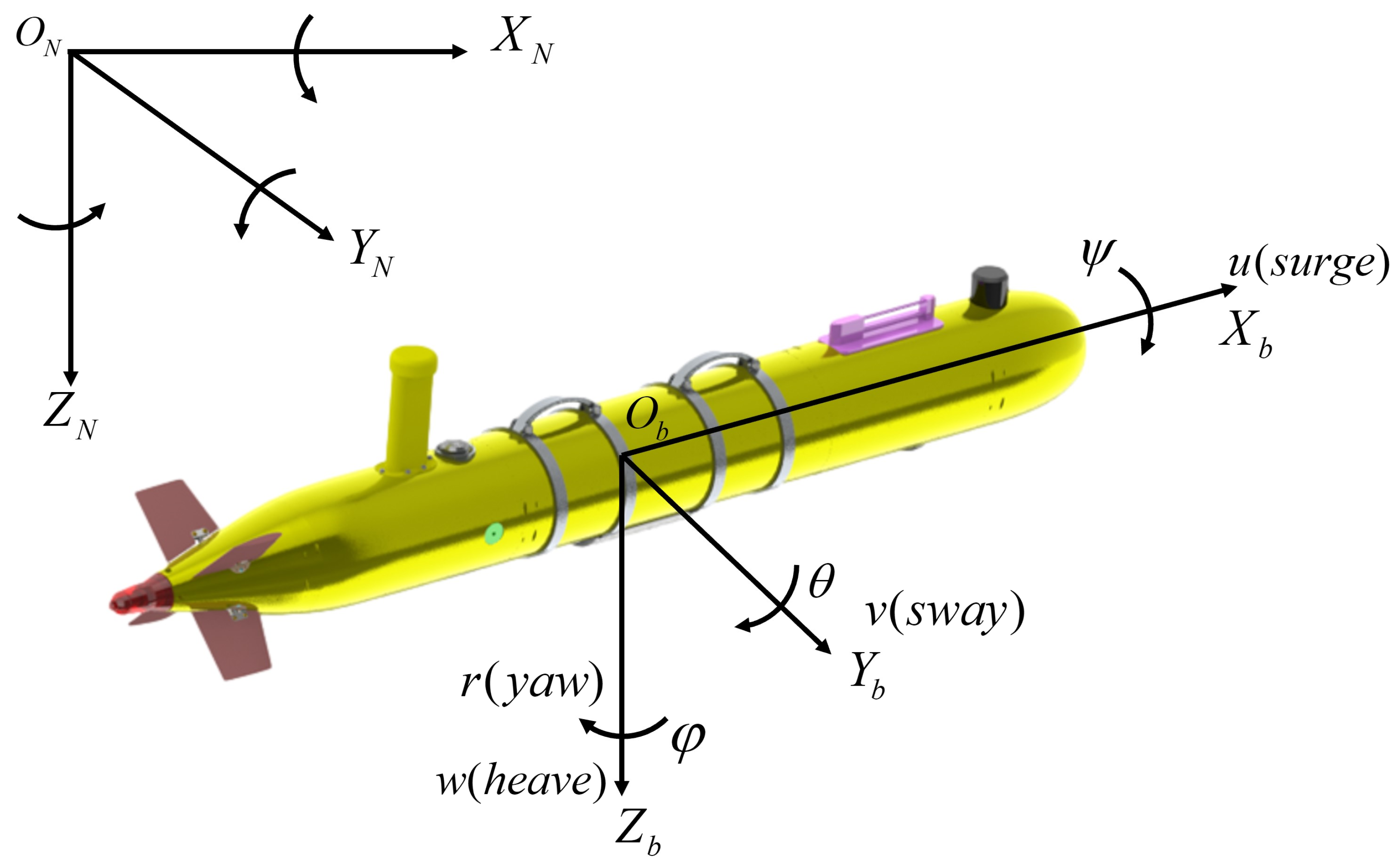
A body-fixed frame $\left\{B\right\}$ is attached to the AUV with origin at $O_b$. The body axes $X_b$, $Y_b$, and $Z_b$ point forward, starboard, and downward, while the NED axes $X_N$, $Y_N$, and $Z_N$ point north, east, and downward. The frames and the Euler angles roll $\varphi$, pitch $\theta$, and yaw $\psi$ are depicted in Figure 1.

The 6-DOF equations of motion comprise the following dynamics and kinematics [18]:

$$\begin{array}{cc}\hfill \mathbf{M}\dot{\mathit{\nu }}+\mathbf{C}\left(\mathit{\nu }\right)\mathit{\nu }+\mathbf{D}\left(\mathit{\nu }\right)\mathit{\nu }+\mathbf{g}\left(\mathit{\eta }\right)& =\mathit{\tau }+{\mathit{\tau }}_e,\hfill \\ \hfill \dot{\mathit{\eta }}& =\mathbf{J}\left(\mathit{\eta }\right)\mathit{\nu }.\hfill \end{array}$$

(1)

Let $\mathit{\eta }={\left[xyz\varphi \theta \psi \right]}^{\mathsf{T}}$ denote the position and attitude in $\left\{N\right\}$, and let $\mathit{\nu }={\left[uvwpqr\right]}^{\mathsf{T}}$ denote the linear and angular velocities in $\left\{B\right\}$. The components u, v, and w are the surge, sway, and heave velocities, and p, q, and r are the roll, pitch, and yaw rates. The generalized input $\mathit{\tau }$ collects actuator-generated forces and moments. The term ${\mathit{\tau }}_e$ represents external loads and unmodeled effects, including wave, wind, and current disturbances.

The system matrices follow the standard decomposition $\mathbf{M}={\mathbf{M}}_{\mathrm{RB}}+{\mathbf{M}}_{\mathrm{A}}$, $\mathbf{C}\left(\mathit{\nu }\right)={\mathbf{C}}_{\mathrm{RB}}\left(\mathit{\nu }\right)+{\mathbf{C}}_{\mathrm{A}}\left(\mathit{\nu }\right)$, and $\mathbf{D}\left(\mathit{\nu }\right)={\mathbf{D}}_{\mathrm{nl}}\left(\mathit{\nu }\right)+{\mathbf{D}}_{\mathrm{Lift}}\left(\mathit{\nu }\right)$, where $\mathrm{RB}$ and $\mathrm{A}$ denote rigid-body and added-mass contributions. The subscript $\mathrm{nl}$ refers to nonlinear drag, while $\mathrm{Lift}$ accounts for lift-induced coupling effects. The restoring vector $\mathbf{g}\left(\mathit{\eta }\right)$ is governed by weight, buoyancy, and their moment arms and therefore varies with the attitude.

For a torpedo-shaped AUV with port–starboard symmetry about the $X_b$–$Z_b$ plane, the coefficient matrices can be represented with the following sparsity structure:

$$\mathbf{M}=\left[\begin{array}{cccccc}{M}_{11}& 0& M_{13}& 0& M_{15}& 0\\ 0& M_{22}& 0& M_{24}& 0& M_{26}\\ M_{13}& 0& M_{33}& 0& M_{35}& 0\\ 0& M_{24}& 0& M_{44}& 0& M_{46}\\ M_{15}& 0& M_{35}& 0& M_{55}& 0\\ 0& M_{26}& 0& M_{46}& 0& M_{66}\end{array}\right].$$

(2)

$$\mathbf{C}\left(\mathit{\nu }\right)=\left[\begin{array}{cccccc}0& 0& 0& C_{14}& C_{15}& C_{16}\\ 0& 0& 0& C_{24}& C_{25}& C_{26}\\ 0& 0& 0& C_{34}& C_{35}& C_{36}\\ C_{41}& C_{42}& C_{43}& 0& C_{45}& C_{46}\\ C_{51}& C_{52}& C_{53}& C_{54}& 0& C_{56}\\ C_{61}& C_{62}& C_{63}& C_{64}& C_{65}& 0\end{array}\right],$$

(3)

$$\mathbf{D}\left(\mathit{\nu }\right)=\left[\begin{array}{cccccc}{D}_{11}& 0& 0& 0& 0& 0\\ 0& D_{22}& 0& 0& 0& D_{26}\\ 0& 0& D_{33}& 0& D_{35}& 0\\ 0& 0& 0& D_{44}& 0& 0\\ 0& 0& D_{53}& 0& D_{55}& 0\\ 0& D_{62}& 0& 0& 0& D_{66}\end{array}\right].$$

(4)

$$\mathbf{g}\left(\mathit{\eta }\right)={\left[\begin{array}{cccccc}{g}_1& g_2& g_3& g_4& g_5& g_6\end{array}\right]}^{\mathsf{T}}.$$

(5)

The kinematic transformation $\mathbf{J}\left(\mathit{\eta }\right)$ maps body-fixed velocities to time rates in the NED frame:

$$\mathbf{J}\left(\mathit{\eta }\right)=\left[\begin{array}{cc}{\mathbf{R}}_{nb}& {\mathbf{0}}_{3\times 3}\\ {\mathbf{0}}_{3\times 3}& \mathbf{T}(\varphi ,\theta )\end{array}\right].$$

(6)

Here, ${\mathbf{R}}_{nb}$ is the direction cosine matrix for the yaw–pitch–roll Euler sequence, and $\mathbf{T}(\varphi ,\theta )$ maps the body angular rate vector to the Euler angle rates.

$${\mathbf{R}}_{nb}=\left[\begin{array}{ccc}\cos \psi \cos \theta & -\sin \psi \cos \varphi +\cos \psi \sin \theta \sin \varphi & \sin \psi \sin \varphi +\cos \psi \sin \theta \cos \varphi \\ \sin \psi \cos \theta & \cos \psi \cos \varphi +\sin \psi \sin \theta \sin \varphi & -\cos \psi \sin \varphi +\sin \psi \sin \theta \cos \varphi \\ -\sin \theta & \cos \theta \sin \varphi & \cos \theta \cos \varphi \end{array}\right],$$

(7)

$$\mathbf{T}(\varphi ,\theta )=\left[\begin{array}{ccc}1& \sin \varphi \tan \theta & \cos \varphi \tan \theta \\ 0& \cos \varphi & -\sin \varphi \\ 0& \sin \varphi /\cos \theta & \cos \varphi /\cos \theta \end{array}\right].$$

(8)

2.2. Actuator Modeling

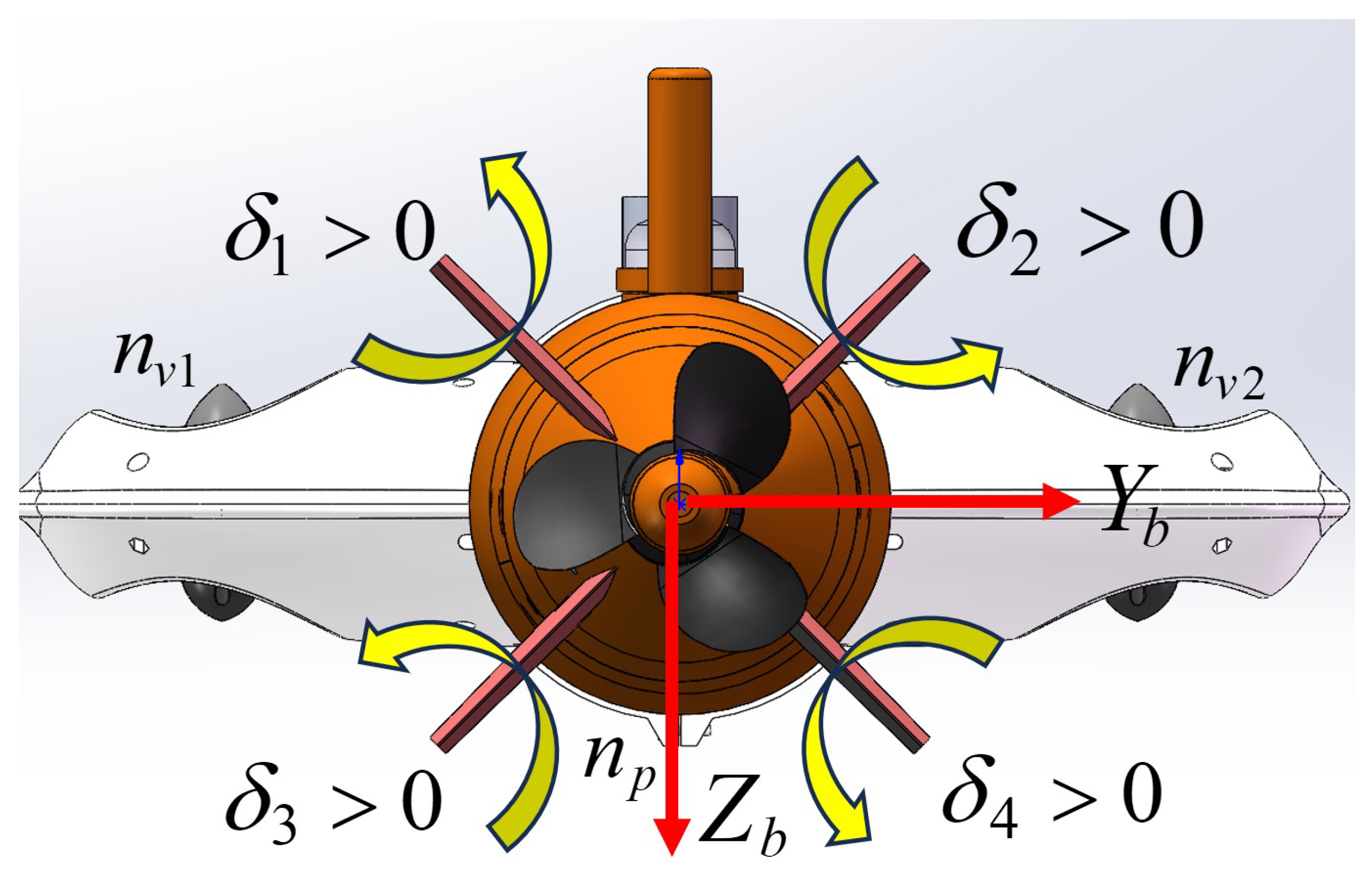
This subsection establishes implementable actuator models for an over-actuated AUV equipped with a stern main propeller, two vertical thrusters, and four independently actuated control surfaces arranged in an X-rudder configuration. The rotation direction of each rudder is shown in Figure 2.

The goal is to obtain explicit and control-oriented relationships between actuator commands and the forces/moments generated by each actuator. The geometric parameters of the T200 propeller and the NACA 0012 rudder are summarized in

Table 1. Geometric parameters of the T200 propeller.

Parameter	Value	Unit
Propeller diameter	0.076	m
Blade pitch angle	22.5	deg
Pitch	0.0704	m
Geometric pitch ratio	0.97	–

and

Table 2. Geometric characteristics of the NACA 0012 rudder.

Parameter	Value	Unit
Airfoil type	NACA 0012	–
Chord length	90	mm
Leading-edge radius	1.575	mm
Trailing-edge angle	16.77	deg
Planform area	10,506.9	${\mathrm{mm}}^2$
Span	116.74	mm
Aspect ratio	1.297	–

, respectively [19].

Let n denote the signed propeller rotational speed (rpm) and let $D_p$ denote the propeller diameter. Define the advance ratio

$$J_p={\displaystyle \frac{V_A}{\left|n\right|D_p}},$$

(9)

where $V_A$ is the local axial inflow speed at the propeller disk. Using conventional open-water coefficients [18], the propeller thrust T and reaction (shaft) torque Q are modeled as

$$T=\rho D_p^4{K}_T\left(J_p\right)n\left|n\right|,Q=\rho D_p^5{K}_Q\left(J_p\right)n\left|n\right|,$$

(10)

where $\rho$ is the water density and $K_T(·)$ and $K_Q(·)$ are the thrust and torque coefficients, respectively.

To avoid overloading the notation $\mathit{\eta }$ used for the pose vector in (1), the propeller efficiency is denoted by ${\eta }_p$ and defined as

$${\eta }_p={\displaystyle \frac{T{V}_A}{2\pi nQ}}={\displaystyle \frac{J_p{K}_T\left(J_p\right)}{2\pi K_Q\left(J_p\right)}}.$$

(11)

On the hardware side, thrusters are typically driven by an ESC using PWM signals. In this work, low-level signal conditioning is treated as an interface-layer detail. The control design and allocation are performed in the thrust domain using T, subject to explicit saturation and rate limits:

$$T_{\min }\le T\le T_{\max },\left|\dot{T}\right|\le {\dot{T}}_{\max }.$$

(12)

In this paper, T is defined as the signed thrust along the actuator force direction $\mathbf{d}$. Therefore, $T_{\max }>0$ corresponds to forward thrust and $T_{\min }<0$ corresponds to reverse thrust for reversible thrusters. For non-reversible devices (or when reverse thrust is disabled), one can set $T_{\min }=0$; the proposed constrained allocator remains applicable with this one-sided bound.

Let ${\delta }_i$ denote the deflection angle of rudder i ($i=1,\dots ,4$). The deflection constraints are modeled as

$${\delta }_{\min }\le {\delta }_i\le {\delta }_{\max },\left|{\dot{\delta }}_i\right|\le {\dot{\delta }}_{\max },i=1,\dots ,4.$$

(13)

For each rudder, the flow-induced force is decomposed into lift $L_i$ and drag $D_i$ with respect to the local inflow. Let $A_r$ denote the reference area of a single rudder surface and let $U_{r,i}$ denote the local relative inflow speed at rudder i. Define the lift and drag coefficients by

$$C_L={\displaystyle \frac{L_i}{\frac{1}{2}\rho A_r{U}_{r,i}^2}},C_D={\displaystyle \frac{D_i}{\frac{1}{2}\rho A_r{U}_{r,i}^2}},i=1,\dots ,4.$$

(14)

Let ${\alpha }_i$ denote the angle of attack of rudder i with respect to the local inflow. Accounting for the local drift angle ${\beta }_i$, we write

$${\alpha }_i={\delta }_i-{\beta }_i,{\beta }_i=\arctan \left({\displaystyle \frac{v_{r,i}}{u_{r,i}}}\right),$$

(15)

where $(u_{r,i},v_{r,i})$ are the local surge and sway components of the inflow at the rudder location. In the low-drift regime considered in this work, ${\beta }_i$ is small and we use the approximation ${\alpha }_i\approx {\delta }_i$.

The lift and drag magnitudes are then given by

$$L_i=\frac{1}{2}\rho U_{r,i}^2{A}_r{C}_L\left({\alpha }_i\right),D_i=\frac{1}{2}\rho U_{r,i}^2{A}_r{C}_D\left({\alpha }_i\right).$$

(16)

To avoid overloading the yaw moment symbol N defined later in (21), the normal force on rudder i is denoted by $F_{N,i}$. The corresponding normal-force coefficient is

$$C_N={\displaystyle \frac{F_{N,i}}{\frac{1}{2}\rho A_r{U}_{r,i}^2}}=C_L\cos {\alpha }_i+C_D\sin {\alpha }_i.$$

(17)

To express the fin force in the body-fixed frame, introduce for each fin a fixed mounting angle ${\lambda }_i$ about $X_b$. Define the body-fixed unit vectors

$${\mathbf{e}}_x={\left[100\right]}^{\mathsf{T}},{\mathbf{e}}_y={\left[010\right]}^{\mathsf{T}},{\mathbf{e}}_z={\left[001\right]}^{\mathsf{T}},$$

(18)

and the unit vector of the lift direction for fin i as

$${\mathbf{e}}_{L_i}={\left[\begin{array}{ccc}0& \cos {\lambda }_i& \sin {\lambda }_i\end{array}\right]}^{\mathsf{T}},i=1,\dots ,4.$$

(19)

The drag acts opposite to the surge direction, i.e., along $-{\mathbf{e}}_x$. Hence, the force generated by fin i in $\left\{B\right\}$ is modeled as

$${\mathbf{f}}_{{\delta }_i}=-D_i{\mathbf{e}}_x+L_i{\mathbf{e}}_{L_i},i=1,\dots ,4.$$

(20)

2.3. Force and Moment Analysis

This subsection converts the actuator force models from Section 2.2 into generalized forces and moments about the body-fixed origin $O_b$, and constructs a control allocation mapping from actuator efforts to the controllable generalized input.

All actuator forces and moments are expressed in the body-fixed frame $\left\{B\right\}$ whose origin is located at $O_b$ and whose axes $(X_b,Y_b,Z_b)$ point forward, starboard, and downward, respectively. Define the generalized force (wrench) vector as

$$\mathit{\tau }={\left[\begin{array}{cccccc}X& Y& Z& K& M& N\end{array}\right]}^{\mathsf{T}}\in {\mathbb{R}}^6,$$

(21)

where $(X,Y,Z)$ are forces along $(X_b,Y_b,Z_b)$ and $(K,M,N)$ are moments about $(X_b,Y_b,Z_b)$.

The vehicle has no dedicated sway actuator; hence, Y is not directly controllable. In the control allocation design, we therefore focus on the five controllable components

$${\mathit{\tau }}_c={\left[\begin{array}{ccccc}X& Z& K& M& N\end{array}\right]}^{\mathsf{T}}\in {\mathbb{R}}^5,$$

(22)

which can be written compactly as ${\mathit{\tau }}_c={\mathbf{S}}_c\mathit{\tau }$ with the constant selection matrix

$${\mathbf{S}}_c=\left[\begin{array}{cccccc}1& 0& 0& 0& 0& 0\\ 0& 0& 1& 0& 0& 0\\ 0& 0& 0& 1& 0& 0\\ 0& 0& 0& 0& 1& 0\\ 0& 0& 0& 0& 0& 1\end{array}\right]\in {\mathbb{R}}^{5\times 6}.$$

(23)

For a generic actuator i located at ${\mathbf{r}}_i={\left[x_i{y}_i{z}_i\right]}^{\mathsf{T}}$ in $\left\{B\right\}$, let ${\mathbf{f}}_i\in {\mathbb{R}}^3$ denote the force applied to the hull. The corresponding generalized force about $O_b$ is

$${\mathit{\tau }}_i=\left[\begin{array}{c}{\mathbf{f}}_i\\ {\mathbf{r}}_i\times {\mathbf{f}}_i\end{array}\right]\in {\mathbb{R}}^6.$$

(24)

If the actuator generates a reaction (shaft) torque about its own axis, this torque is added to the moment part of ${\mathit{\tau }}_i$.

Let $\mathcal{T}$ denote the set of thrusters. For a thruster $j\in \mathcal{T}$, define its unit force direction ${\mathbf{d}}_j$ and thrust magnitude $T_j$. Then, ${\mathbf{f}}_j=T_j{\mathbf{d}}_j$. If shaft torque $M_j$ is modeled, its contribution is $M_j{\mathbf{d}}_j$ in the moment part. Thus,

$${\mathit{\tau }}_j=\left[\begin{array}{c}{T}_j{\mathbf{d}}_j\\ {\mathbf{r}}_j\times \left(T_j{\mathbf{d}}_j\right)+M_j{\mathbf{d}}_j\end{array}\right],j\in \mathcal{T}.$$

(25)

For rudder i, the body-fixed force ${\mathbf{f}}_{{\delta }_i}$ is given in (20). The corresponding generalized force contribution is

$${\mathit{\tau }}_{{\delta }_i}=\left[\begin{array}{c}{\mathbf{f}}_{{\delta }_i}\\ {\mathbf{r}}_{{\delta }_i}\times {\mathbf{f}}_{{\delta }_i}\end{array}\right],i=1,\dots ,4,$$

(26)

where ${\mathbf{r}}_{{\delta }_i}$ is the position vector of rudder i relative to $O_b$.

The total actuator-generated generalized force is the sum of all thruster and rudder contributions:

$$\mathit{\tau }=\sum _{j\in \mathcal{T}}{\mathit{\tau }}_j+\sum _{i=1}^4{\mathit{\tau }}_{{\delta }_i}.$$

(27)

For control allocation, define the actuator effort vector

$${\mathit{u}}_a={\left[\begin{array}{ccccccc}{T}_{v1}& T_{v2}& T_p& L_1& L_2& L_3& L_4\end{array}\right]}^{\mathsf{T}}\in {\mathbb{R}}^7,$$

(28)

where $T_{v1}$ and $T_{v2}$ are the thrusts of the port and starboard vertical thrusters, $T_p$ is the main propeller thrust, and $L_i$ is the lift generated by rudder i. This choice yields a linear mapping in ${\mathit{u}}_a$ with a geometry-dependent configuration matrix. The lift variables $L_i$ remain physically implementable through the rudder model (16) by enforcing the corresponding deflection constraints (13).

Assuming fixed actuator mounting directions and geometry, the linear mapping from ${\mathit{u}}_a$ to the controllable generalized input ${\mathit{\tau }}_c$ can be written as

$${\mathit{\tau }}_c=\mathbf{B}{\mathit{u}}_a+{\mathit{\tau }}_{\mathrm{drag}}+{\mathit{\tau }}_{\mathrm{shaft}},$$

(29)

where $\mathbf{B}\in {\mathbb{R}}^{5\times 7}$ is the actuator configuration matrix, ${\mathit{\tau }}_{\mathrm{drag}}$ collects drag-induced surge losses and associated moments, and ${\mathit{\tau }}_{\mathrm{shaft}}$ collects propeller reaction torques.

A convenient explicit construction is obtained by separating the lift-related terms from drag and shaft-torque terms. Let ${\mathbf{d}}_{v1},{\mathbf{d}}_{v2},{\mathbf{d}}_p$ denote the unit thrust directions and ${\mathbf{r}}_{v1},{\mathbf{r}}_{v2},{\mathbf{r}}_p$ their position vectors w.r.t. $O_b$. Then,

$$\mathbf{B}={\mathbf{S}}_c\left[\begin{array}{ccccccc}{\mathbf{d}}_{v1}& {\mathbf{d}}_{v2}& {\mathbf{d}}_p& {\mathbf{e}}_{L_1}& {\mathbf{e}}_{L_2}& {\mathbf{e}}_{L_3}& {\mathbf{e}}_{L_4}\\ {\mathbf{r}}_{v1}\times {\mathbf{d}}_{v1}& {\mathbf{r}}_{v2}\times {\mathbf{d}}_{v2}& {\mathbf{r}}_p\times {\mathbf{d}}_p& {\mathbf{r}}_{{\delta }_1}\times {\mathbf{e}}_{L_1}& {\mathbf{r}}_{{\delta }_2}\times {\mathbf{e}}_{L_2}& {\mathbf{r}}_{{\delta }_3}\times {\mathbf{e}}_{L_3}& {\mathbf{r}}_{{\delta }_4}\times {\mathbf{e}}_{L_4}\end{array}\right].$$

(30)

The drag-induced term resulting from $-D_i{\mathbf{e}}_x$ in (20) is collected as

$${\mathit{\tau }}_{\mathrm{drag}}={\mathbf{S}}_c\sum _{i=1}^4\left[\begin{array}{c}-D_i{\mathbf{e}}_x\\ {\mathbf{r}}_{{\delta }_i}\times (-D_i{\mathbf{e}}_x)\end{array}\right],$$

(31)

and the shaft-torque term is collected as

$${\mathit{\tau }}_{\mathrm{shaft}}={\mathbf{S}}_c\sum _{j\in \mathcal{T}}\left[\begin{array}{c}{\mathbf{0}}_{3\times 1}\\ M_j{\mathbf{d}}_j\end{array}\right].$$

(32)

Thruster constraints are enforced directly in the thrust domain via (12). For rudders, the physical limits are naturally expressed in terms of ${\delta }_i$ and ${\dot{\delta }}_i$ in (13). If ${\mathit{u}}_a$ uses $L_i$ as decision variables (as in (28)), the corresponding feasible bounds on $L_i$ can be obtained online from the current inflow $U_{r,i}$ and the lift map (16) by evaluating $L_i\left({\delta }_{\min }\right)$ and $L_i\left({\delta }_{\max }\right)$. In the subsequent constrained control allocation design, ${\mathit{\tau }}_{\mathrm{drag}}$ and ${\mathit{\tau }}_{\mathrm{shaft}}$ are treated as secondary effects and are either compensated or penalized through the optimization objective.

2.4. Test Framework

This study adopts MOOS-IvP 24.8 as the software backbone of the test framework. MOOS-IvP is an open-source, cross-platform middleware suite for marine autonomy [20]. At its core, the MOOS database (MOOSDB) implements a publish–subscribe communication mechanism that supports real-time, time-stamped data exchange among distributed autonomy processes running on the payload computer. Within the MOOS-IvP ecosystem, IvP-Helm complements the MOOS middleware as the autonomy engine and follows a behavior-based decision architecture. At each iteration, IvP-Helm constructs and solves an IvP objective function, and it arbitrates among mission behaviors by priority to coordinate commands such as desired speed and desired depth.

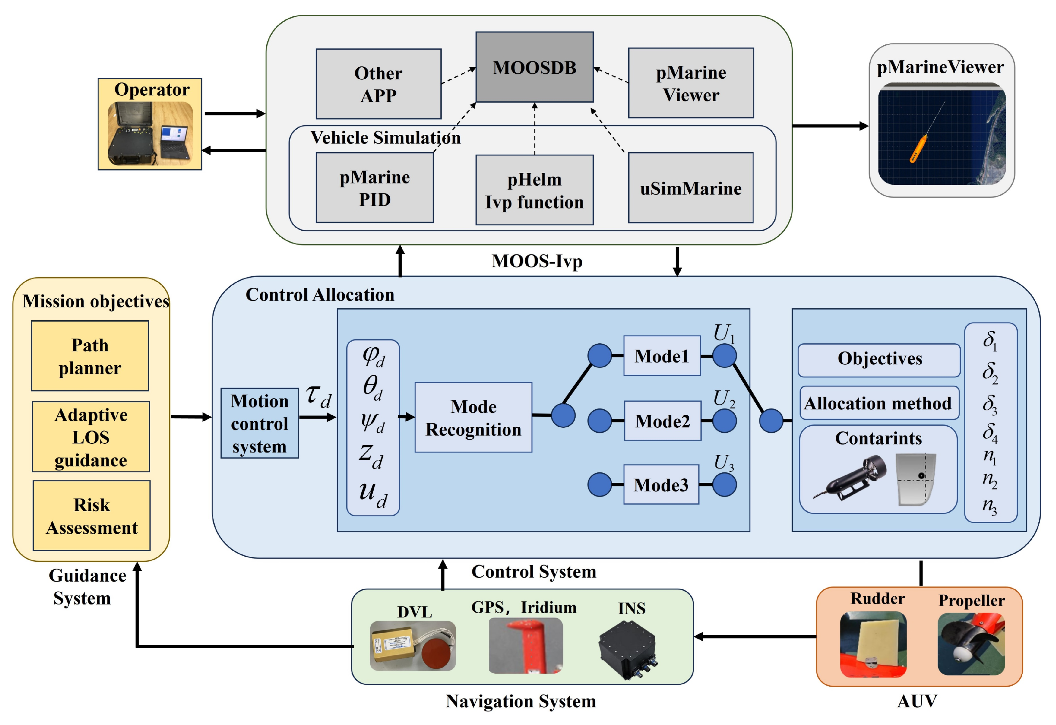
As shown in Figure 3, the closed-loop test platform is organized around MOOSDB, which interconnects the main controller, the multi-mode control allocator, the vehicle simulator, and visualization/logging utilities.

In the control loop, the guidance subsystem outputs the motion references required by the mission. This work employs an adaptive line-of-sight guidance (ALOS) law to generate desired heading and desired depth references [21]. The motion-control layer applies adaptive PID controllers in the horizontal and vertical planes to track these references and then outputs a virtual generalized force and moment command that is to be realized by the actuators.

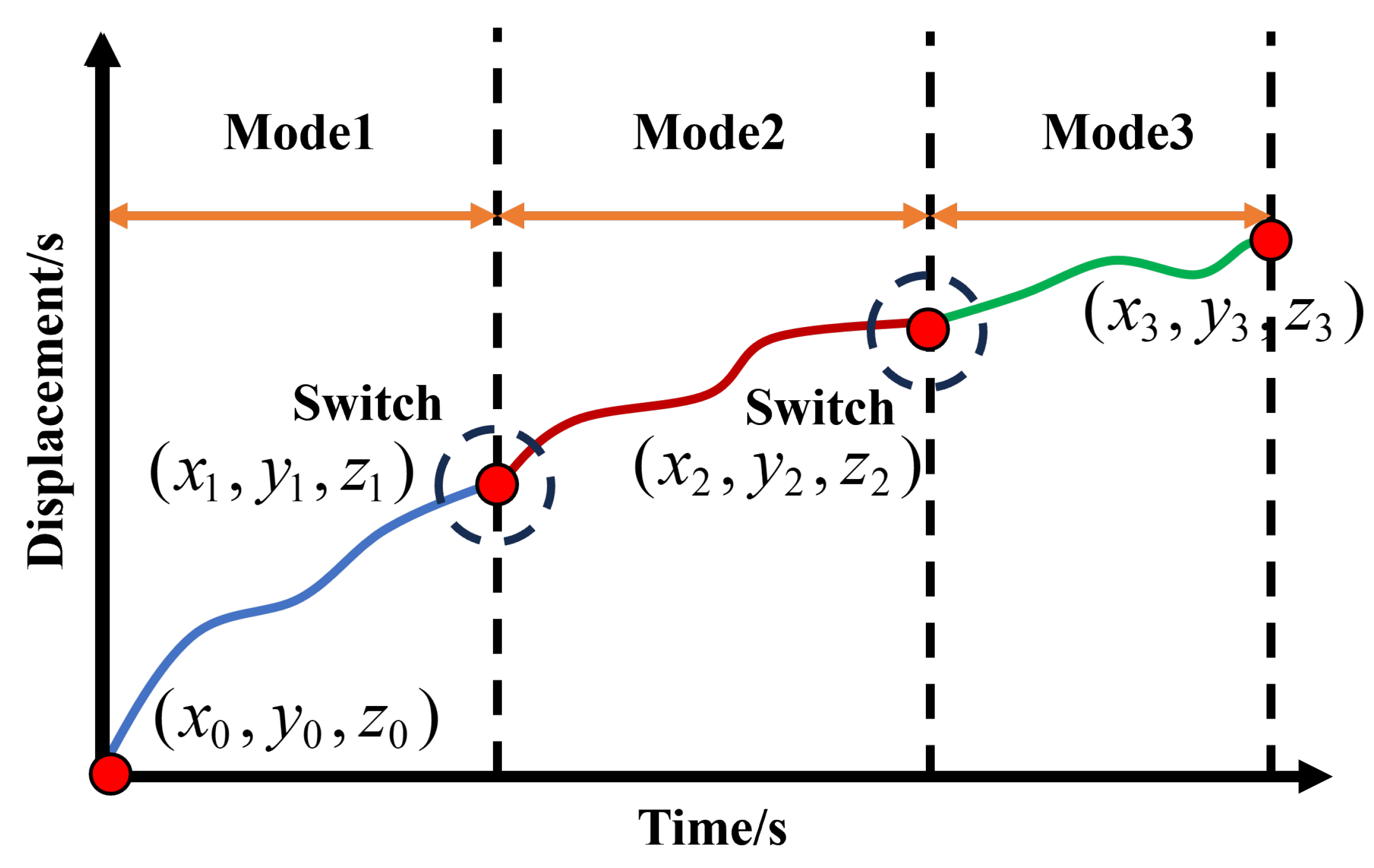
To accommodate the forward, reverse, and hover modes commonly encountered in docking-and-seating tasks, the system introduces a smooth multi-mode switching mechanism.

The control allocation module is the core of this study. At each cycle, a unified SQP routine generates actuator set points for the main propeller, vertical thrusters, and X-type rudders. The next section details this multi-mode control allocation method.

3. Methodology

3.1. Attainable Force and Moment Set Analysis

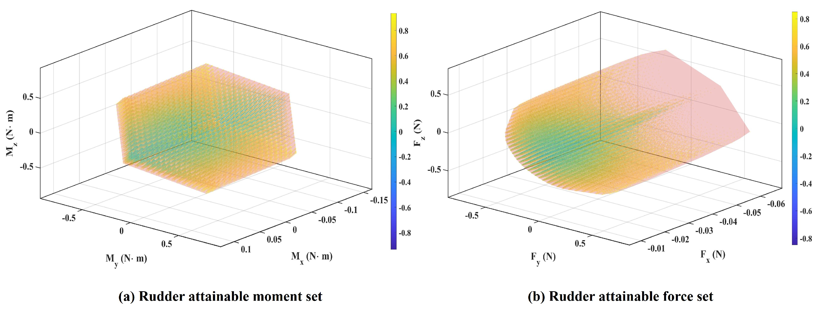
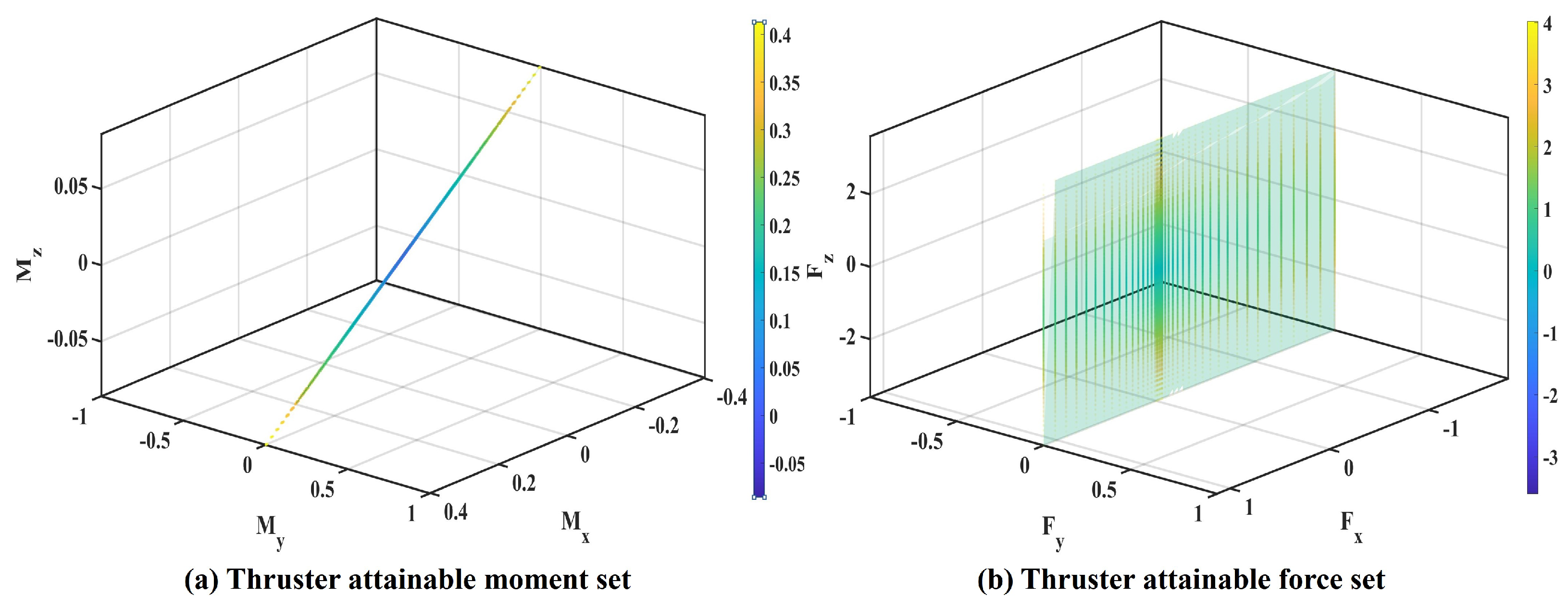
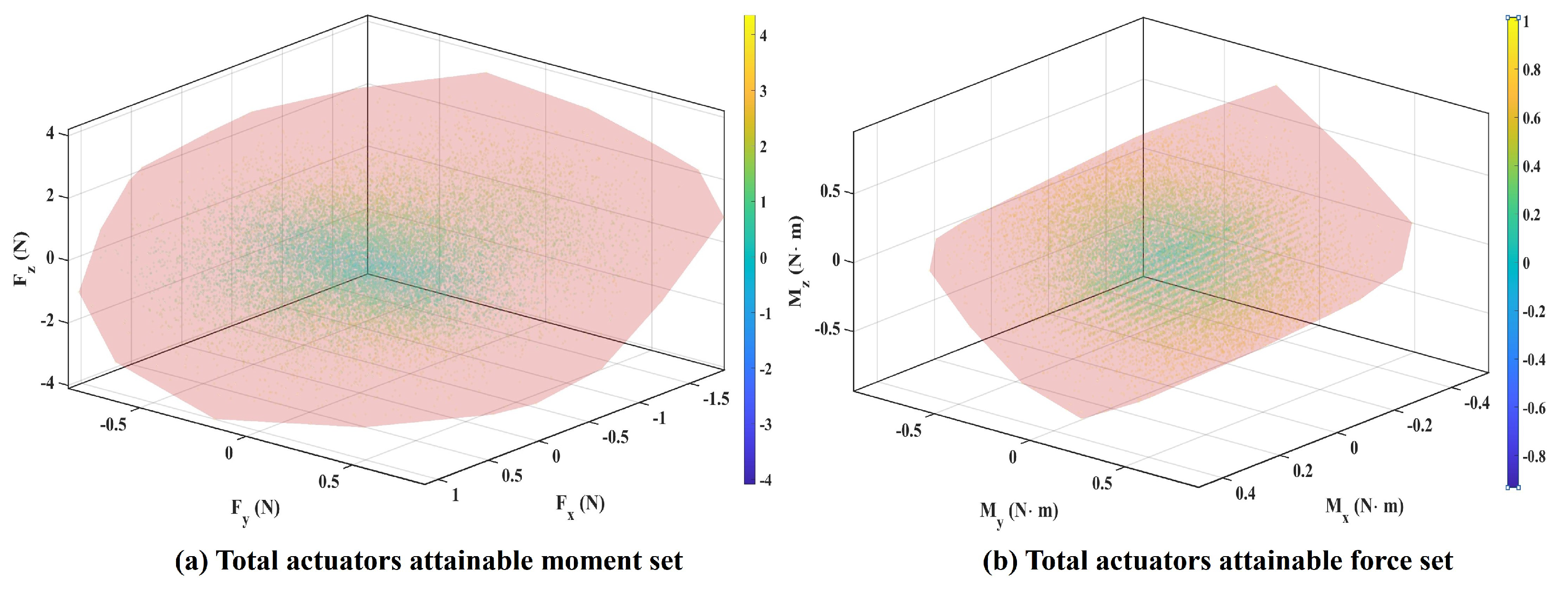
This subsection analyzes actuator saturation for the over-actuated AUV equipped with four X-type rudders, one stern main propeller, and two vertical thrusters. We use the attainable force set (AFS) and the attainable moment set (AMS) to describe the realizable force and moment outputs under actuator limits. The analysis is conducted at a representative low-speed condition $u=0.2\mathrm{m}/\mathrm{s}$. Figure 4, Figure 5 and Figure 6 illustrate the attainable envelopes of the rudder-only subsystem, the thruster-only subsystem, and the full actuator suite, and

Table 3. AFS/AMS geometric indicators for various actuator configurations at $u=0.2\mathrm{m}/\mathrm{s}$.

Configuration	Force Volume	Force Surface Area	Moment Volume	Moment Surface Area
Rudder	0.0693	3.0142	0.2566	3.9351
Thrusters	–	21.1197	–	0.0012
Total actuators	31.8633	68.3097	1.4329	6.9633

reports the associated geometric metrics.

The actuator models established in Section 2.2 map the actuator commands to the generalized wrench $\mathit{\tau }$ defined in (21). In this subsection, we focus on the force and moment parts of $\mathit{\tau }$, denoted by

$${\mathit{\tau }}_F={\left[\begin{array}{ccc}X& Y& Z\end{array}\right]}^{\mathsf{T}}\in {\mathbb{R}}^3,{\mathit{\tau }}_M={\left[\begin{array}{ccc}K& M& N\end{array}\right]}^{\mathsf{T}}\in {\mathbb{R}}^3,$$

(33)

where ${\mathit{\tau }}_F$ corresponds to $(F_x,F_y,F_z)$ in the AFS plots and ${\mathit{\tau }}_M$ corresponds to $(M_x,M_y,M_z)$ in the AMS plots.

To distinguish it from the scalar surge speed u in the 6-DOF model, the actuator command vector is denoted by $\mathbf{u}$:

$$\mathit{u}={\left[\begin{array}{cc}{\mathit{\delta }}^{\mathsf{T}}& {\mathit{n}}^{\mathsf{T}}\end{array}\right]}^{\mathsf{T}}\in {\mathbb{R}}^7,\mathit{\delta }={\left[\begin{array}{cccc}{\delta }_1& {\delta }_2& {\delta }_3& {\delta }_4\end{array}\right]}^{\mathsf{T}},\mathit{n}={\left[\begin{array}{ccc}{n}_p& n_{v1}& n_{v2}\end{array}\right]}^{\mathsf{T}},$$

(34)

where ${\delta }_i$ is the deflection angle of rudder i, and $n_p$, $n_{v1}$, and $n_{v2}$ are the signed rotational speeds of the main propeller and the two vertical thrusters. The admissible command set is:

$${\mathcal{U}}_{\mathrm{cmd}}=\left\{\mathit{u}\in {\mathbb{R}}^7|{\delta }_i\in [{\delta }_{\min },{\delta }_{\max }],i=1,\dots ,4;n_j\in [n_{\min },n_{\max }],j\in \{p,v1,v2\}\right\}$$

(35)

with ${\delta }_{\max }={15}^{°}$ and $n_{\max }=200\mathrm{rpm}$.

Using the actuator models, the force and moment outputs are expressed as nonlinear mappings:

$${\mathit{\tau }}_F={\mathcal{G}}_F(\mathit{u};u),{\mathit{\tau }}_M={\mathcal{G}}_M(\mathit{u};u).$$

(36)

The attainable force set and attainable moment set are then defined as

$$\mathrm{AFS}\left(u\right)=\left\{{\mathit{\tau }}_F\in {\mathbb{R}}^3|{\mathit{\tau }}_F={\mathcal{G}}_F(\mathit{u};u),\mathit{u}\in {\mathcal{U}}_{\mathrm{cmd}}\right\},$$

(37)

$$\mathrm{AMS}\left(u\right)=\left\{{\mathit{\tau }}_M\in {\mathbb{R}}^3|{\mathit{\tau }}_M={\mathcal{G}}_M(\mathit{u};u),\mathit{u}\in {\mathcal{U}}_{\mathrm{cmd}}\right\}.$$

(38)

Their boundaries, $\partial \mathrm{AFS}\left(u\right)$ and $\partial \mathrm{AMS}\left(u\right)$, form the saturation envelopes in force and moment spaces.

Because the rudder lift/drag depends on deflection and the thruster outputs follow nonlinear static maps, ${\mathcal{G}}_F(·)$ and ${\mathcal{G}}_M(·)$ are nonlinear. We therefore estimate $\mathrm{AFS}\left(u\right)$ and $\mathrm{AMS}\left(u\right)$ by sampling. Each rudder deflection is discretized into 20 levels over $\pm {15}^{°}$, and each thruster speed is discretized into 100 levels over $\pm 200\mathrm{rpm}$. For the full seven-dimensional command vector, we use 20,000 random samples to approximate the joint envelope. Each sample yields a force vector and a moment vector, which together form point clouds in ${\mathbb{R}}^3$. We compute a convex-hull approximation of the sampled point cloud and evaluate its volume and surface area as compact indicators (Table 3); this approximation depends on the sampling density and does not necessarily represent the exact nonconvex boundary.

Figure 4 shows the rudder-only envelopes. The rudder AMS forms a bounded three-dimensional set, but it expands less along the roll axis than along the pitch and yaw axes. The rudder AFS is asymmetric in surge and shifts toward negative surge force. The rudders mainly generate lateral and vertical forces through lift, and they introduce drag rather than positive surge thrust. This feature becomes more pronounced as the vehicle slows down because the rudder effectiveness decreases with dynamic pressure.

Figure 5 shows the thruster-only envelopes. The thruster AFS is close to a plane because the configuration produces negligible direct sway force. It mainly spans surge and heave forces. The thruster AMS collapses to an almost one-dimensional segment, which indicates that the thruster-generated moments remain strongly coupled under fixed mounting directions and fixed geometry. Thrusters alone therefore cannot span a full three-axis moment envelope, even though they can generate large force magnitudes.

Figure 6 shows the envelopes of the full actuator suite. The combined AFS and AMS become fully three-dimensional and cover directions that are missing in the rudder-only and thruster-only cases. The rudders enlarge the attainable moment directions, while the thrusters enlarge the attainable force magnitudes. The combined envelopes reflect the complementary roles of the two actuator groups at low speed.

The envelope characteristics align with the three mission modes considered in this work. In forward mode, the vehicle tracks positive surge while regulating attitude; the rudders efficiently generate pitch and yaw moments, but large deflections increase drag and reduce surge efficiency. In reverse mode, the vehicle demands negative surge during braking while maintaining attitude stability; the thrusters generate reverse surge and heave forces without relying on drag, and the rudders maintain pitch and yaw authority as the surge force changes sign. In hover mode, the vehicle requires strong heave with near-zero surge; the vertical thrusters dominate heave force and can create roll moments through differential thrust, whereas the remaining moment directions stay limited in the thruster-only envelope. The vehicle therefore relies on the rudders to maintain a three-axis attainable moment envelope at low speed, which is consistent with the total actuator AMS shown in Figure 6.

3.2. Motion-Control System

This paper follows the standard layered structure used for marine craft motion control [18], where a guidance module generates kinematic references and a motion controller converts them into a desired generalized force and moment command for control allocation. This organization is consistent with the guidance–control allocation framework commonly adopted in marine guidance and autopilot systems. The output of this layer is the desired controllable wrench

$${\mathit{\tau }}_d={\left[\begin{array}{ccccc}{X}_d& Z_d& K_d& M_d& N_d\end{array}\right]}^{\mathsf{T}}\in {\mathbb{R}}^5,$$

(39)

which corresponds to the five controllable components defined in (22).

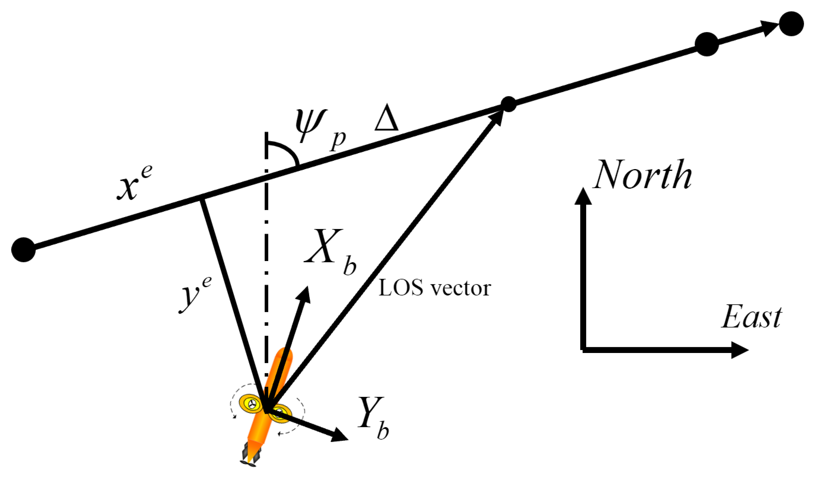
As shown in Figure 7, the guidance module provides the reference signals $u_d$, $z_d$, and ${\psi }_d$. For the docking-and-seating experiments, the attitude references are set to ${\varphi }_d=0$ and ${\theta }_d=0$.

The desired heading ${\psi }_d$ is generated by adaptive line-of-sight guidance, abbreviated as ALOS [21]. Let $y_e$ denote the horizontal cross-track error, let $\Delta >0$ denote the look-ahead distance, and let ${\psi }_p$ denote the path-tangential heading. A bias term $\widehat{b}$ is introduced to compensate slowly varying lateral effects such as current-induced drift. The guidance law is written as

$${\psi }_d={\psi }_p-\arctan \left({\displaystyle \frac{y_e+\widehat{b}}{\Delta }}\right),$$

(40)

and the bias estimate is updated by a simple adaptation law

$$\dot{\widehat{b}}=\gamma y_e,$$

(41)

where $\gamma >0$ is an adaptation gain. The depth reference $z_d$ is generated using the same look-ahead principle in the vertical plane, yielding smooth depth commands during low-speed operations.

Given the navigation estimates $\mathit{\eta }$ and $\mathit{\nu }$, the motion controller applies a diagonal PID structure with standard implementation details for discrete-time execution, including anti-windup handling for actuator saturation and bumpless transfer during mode changes [22,23]. Define the tracking error vector

$$\mathit{e}={\left[\begin{array}{ccccc}{u}_d-u& z_d-z& {\varphi }_d-\varphi & {\theta }_d-\theta & {\psi }_d-\psi \end{array}\right]}^{\mathsf{T}},$$

(42)

and an integral state ${\mathit{e}}_I$ governed by ${\dot{\mathit{e}}}_I=\mathit{e}$ with standard integral limiting. The desired controllable wrench is computed as

$${\mathit{\tau }}_d={\mathbf{K}}_P\mathit{e}+{\mathbf{K}}_I{\mathit{e}}_I+{\mathbf{K}}_D\dot{\mathit{e}},$$

(43)

where ${\mathbf{K}}_P$, ${\mathbf{K}}_I$, and ${\mathbf{K}}_D$ are diagonal gain matrices and are scheduled by the operating condition to account for the change in control effectiveness at low speed. The resulting ${\mathit{\tau }}_d$ is passed to the multi-mode control allocation module, which computes feasible actuator set points under saturation and rate constraints.

3.3. Multi-Mode Control Allocation

This subsection presents a mode-driven control allocation (MD-CA) framework (Figure 8) that unifies (i) mode switching and (ii) constrained allocation within a single SQP layer [24]. At each control cycle k, the motion-control layer provides the desired controllable wrench ${\mathit{\tau }}_d\left(k\right)\in {\mathbb{R}}^5$. The allocator computes the actuator command vector $\mathit{u}\left(k\right)\in {\mathbb{R}}^7$ under amplitude and increment constraints while trading off wrench tracking and actuator usage; command smoothness is enforced explicitly by an increment bound [7,25].

The scalar surge speed u in the 6-DOF model is distinct from the actuator command vector $\mathit{u}(·)$. To reduce index clutter, we suppress the time index k in the allocation problem and the SQP iterations: for a given cycle, let the current mode be $m:={\sigma }_k\in \mathcal{S}$ and define

$${\mathit{\tau }}_d:={\mathit{\tau }}_d\left(k\right),{\mathit{u}}^{-}:=\mathit{u}(k-1),\mathit{u}:=\mathit{u}\left(k\right).$$

All mode-dependent weights and bounds are selected by m (and may be smoothly scheduled during switching); the explicit dependence is omitted when unambiguous.

Let the discrete mode variable ${\sigma }_k$ take values in

$$\mathcal{S}=\left\{\mathrm{F},\mathrm{R},\mathrm{H}\right\},$$

(44)

corresponding to forward cruise (F), reverse approach (R), and hover observation (H), respectively.

To accommodate mode-dependent nonlinear actuation effectiveness [9,26], we describe the realized controllable wrench by a continuously differentiable mapping

$${\mathit{\tau }}_c={\mathcal{G}}_m\left(\mathit{u}\right).$$

(45)

When a local affine approximation is sufficient, we use the SQP linearization in (50) and write

$${\mathit{\tau }}_c\approx {\mathcal{G}}_m\left({\mathit{u}}_j\right)+{\mathbf{G}}_j(\mathit{u}-{\mathit{u}}_j)={\mathbf{B}}_{m,j}\mathit{u}+{\mathit{b}}_{m,j},$$

(46)

where ${\mathbf{B}}_{m,j}:={\mathbf{G}}_j$ and ${\mathit{b}}_{m,j}:={\mathcal{G}}_m\left({\mathit{u}}_j\right)-{\mathbf{G}}_j{\mathit{u}}_j$ are updated online at each SQP iteration.

In this work, ${\mathcal{G}}_m(·)$ is constructed by composing the actuator static models in Section 2.2 with the wrench assembly in (27) and the controllable component selection in (22).

We define the weighted quadratic form ${\parallel x\parallel }_{\mathbf{W}}^2=x^{\mathsf{T}}\mathbf{W}x$ for a symmetric positive semidefinite $\mathbf{W}$.

At each cycle, given ${\mathit{\tau }}_d$ and the previous solution ${\mathit{u}}^{-}$, the allocator solves the mode-parameterized problem

$$\mathit{u}=\arg \underset{\mathit{u}\in {\mathbb{R}}^7}{\min }{∥{\mathit{\tau }}_d-{\mathcal{G}}_m\left(\mathit{u}\right)∥}_{\mathbf{Q}}^2+\lambda {∥\mathit{u}∥}_{\mathbf{R}}^2,$$

(47)

subject to the element-wise amplitude and increment bounds

$${\mathit{u}}_{\min }\le \mathit{u}\le {\mathit{u}}_{\max },-\Delta {\mathit{u}}_{\max }\le \mathit{u}-{\mathit{u}}^{-}\le \Delta {\mathit{u}}_{\max }.$$

(48)

Here, $\mathbf{Q}\in {\mathbb{R}}^{5\times 5}$ prioritizes controllable wrench components, $\mathbf{R}\in {\mathbb{R}}^{7\times 7}$ penalizes actuator usage as a convex proxy of energy and wear, $\lambda \ge 0$ is a (mode-dependent) tradeoff coefficient, and $\Delta {\mathit{u}}_{\max }:={\dot{\mathit{u}}}_{\max }\Delta t$ is the per-cycle command increment bound.

Problem (47)–(48) is a small nonlinear constrained least-squares problem. We solve it using an SQP method warm-started from the previous solution [27]. Let $\mathcal{U}$ denote the feasible set induced by (48) for the current cycle and initialize

$${\mathit{u}}_0={\mathrm{\Pi }}_{\mathcal{U}}\left({\mathit{u}}^{-}\right).$$

(49)

At SQP iteration j, linearize the wrench map around the current iterate ${\mathbf{u}}_j$:

$${\mathcal{G}}_m\left({\mathit{u}}_j+\Delta \mathit{u}\right)\approx {\mathcal{G}}_m\left({\mathit{u}}_j\right)+{\mathbf{G}}_j\Delta \mathit{u},{\mathbf{G}}_j\triangleq {\left.{\displaystyle \frac{\partial {\mathcal{G}}_m}{\partial \mathit{u}}}\right|}_{\mathit{u}={\mathit{u}}_j}.$$

(50)

Let the residual be ${\mathit{r}}_j\triangleq {\mathit{\tau }}_d-{\mathcal{G}}_m\left({\mathit{u}}_j\right)$. Using a Gauss–Newton approximation of the Hessian, each SQP step solves the convex QP subproblem

$$\begin{array}{cc}\hfill \Delta {\mathit{u}}_j=\arg \underset{\Delta \mathit{u}\in {\mathbb{R}}^7}{\min }& {∥{\mathit{r}}_j-{\mathbf{G}}_j\Delta \mathit{u}∥}_{\mathbf{Q}}^2+\lambda {∥{\mathit{u}}_j+\Delta \mathit{u}∥}_{\mathbf{R}}^2\hfill \\ \hfill \mathrm{s}.\mathrm{t}.& {\mathit{u}}_j+\Delta \mathit{u}\in \mathcal{U}.\hfill \end{array}$$

(51)

We then update

$${\mathit{u}}_{j+1}={\mathrm{\Pi }}_{\mathcal{U}}\left({\mathit{u}}_j+{\eta }_j\Delta {\mathit{u}}_j\right),{\eta }_j\in (0,1].$$

(52)

In real-time implementation, we use a small fixed iteration budget with warm-starting to guarantee a deterministic runtime. When ${\mathcal{G}}_m(·)$ is affine, the SQP method converges in one iteration and (51) recovers the original convex QP allocation.

Forward–reverse–hover allocation laws previously written as separate optimization problems are recovered as special cases of (47)–(48) by selecting the mode parameters $\{{\mathcal{G}}_m,\mathbf{Q},\mathbf{R},\lambda ,{\mathit{u}}_{\min },{\mathit{u}}_{\max },\Delta {\mathit{u}}_{\max }\}$.

We now reintroduce the time index k for the mode supervisor. Let $d_k\ge 0$ denote the estimated range-to-target (or range-to-observation point), and let ${\chi }_k\in \{0,1\}$ be a target detection flag (${\chi }_k=1$ if the target is detected with sufficient confidence). The supervisor updates the mode ${\sigma }_k\in \mathcal{S}$ using guard conditions based only on $(d_k,{\chi }_k)$.

We use hysteresis thresholds and enforce a minimum dwell time of $N_{\mathrm{dwell}}$ cycles between switches [28]. Let $k_s$ be the index of the most recent switch. For compactness, define the lower/upper thresholds

$$d_{RH}^L,d_{RH}^U,d_{FR}^L,d_{FR}^U,d_{HF}^U,$$

with ordering

$$d_{RH}^L<d_{RH}^U<d_{FR}^L<d_{FR}^U<d_{HF}^U.$$

Then, the mode update logic is

$${\sigma }_{k+1}=\left\{\begin{array}{cc}{\sigma }_k,\hfill & k-k_s<N_{\mathrm{dwell}},\hfill \\ \mathrm{R},\hfill & {\sigma }_k=\mathrm{F},{\chi }_k=1,d_k\le d_{FR}^L,\hfill \\ \mathrm{H},\hfill & {\sigma }_k=\mathrm{R},{\chi }_k=1,d_k\le d_{RH}^L,\hfill \\ \mathrm{F},\hfill & {\sigma }_k=\mathrm{R},({\chi }_k=0\vee d_k\ge d_{FR}^U),\hfill \\ \mathrm{R},\hfill & {\sigma }_k=\mathrm{H},{\chi }_k=1,d_k\ge d_{RH}^U,\hfill \\ \mathrm{F},\hfill & {\sigma }_k=\mathrm{H},({\chi }_k=0\vee d_k\ge d_{HF}^U),\hfill \\ {\sigma }_k,\hfill & \mathrm{otherwise}.\hfill \end{array}\right.$$

(53)

The hysteresis prevents chattering near thresholds, and the dwell time logic implements an average dwell time (ADT) bound.

3.4. Bumpless Mode Switching

Hard switching of the desired wrench and the SQP data may introduce transients [4,5,6,29]. Related bumpless transfer results for switched systems also include transition-dependent and ADT-based designs [30,31,32]. We apply three complementary mechanisms.

Throughout this subsection, we keep the explicit cycle index only in the ramp definition (54); all other quantities refer to the current cycle. Let $k_s$ denote the switching instant, with pre-switch mode $m^{-}$ and post-switch mode $m^{+}$. For any mode-dependent quantity q, we use the shorthand $q^{-}:=q_{m^{-}}$ and $q^{+}:=q_{m^{+}}$.

(1) Continuous scheduling. We compute a transition factor $\kappa \in [0,1]$ ramped over $N_{\mathrm{sw}}$ cycles [6,33]:

$$\kappa =\mathrm{sat}\left({\displaystyle \frac{k-k_s}{N_{\mathrm{sw}}}}\right),\mathrm{sat}\left(x\right):=\min \{1,\max \{0,x\}\},k\ge k_s.$$

(54)

The desired wrench and the key SQP weights are then scheduled by convex interpolation:

$$\begin{array}{cc}\hfill {\mathit{\tau }}_d& =(1-\kappa ){\mathit{\tau }}_d^{-}+\kappa {\mathit{\tau }}_d^{+},\hfill \\ \hfill \mathbf{Q}& =(1-\kappa ){\mathbf{Q}}^{-}+\kappa {\mathbf{Q}}^{+},\hfill \\ \hfill \mathbf{R}& =(1-\kappa ){\mathbf{R}}^{-}+\kappa {\mathbf{R}}^{+},\hfill \\ \hfill \lambda & =(1-\kappa ){\lambda }^{-}+\kappa {\lambda }^{+}.\hfill \end{array}$$

(55)

This removes step changes in the commanded wrench and in the dominant optimization weights.

(2) Integrator alignment (bumpless PID). If the motion-control layer uses mode-dependent PID gains for a channel [5,6,34], ${\mathit{\tau }}_d={\mathbf{K}}_P\mathit{e}+{\mathbf{K}}_I{\mathit{e}}_I+{\mathbf{K}}_D\dot{\mathit{e}}$, then at $k=k_s$ we reset the integrator state to keep the PID output continuous:

$${\mathit{e}}_I^{+}={\left({\mathbf{K}}_I^{+}\right)}^{-1}\left({\mathit{\tau }}_{\mathrm{eq}}-{\mathbf{K}}_P^{+}{\mathit{e}}_s-{\mathbf{K}}_D^{+}{\dot{\mathit{e}}}_s\right),$$

(56)

where ${\mathit{e}}_s:=\mathit{e}\left(k_s\right)$ and ${\dot{\mathit{e}}}_s:=\dot{\mathit{e}}\left(k_s\right)$. Let ${\mathit{u}}^{-}$ denote the command applied in the previous cycle, in particular, at switching ${\mathit{u}}^{-}=\mathit{u}(k_s-1)$. We choose ${\mathit{\tau }}_{\mathrm{eq}}$ as the pre-switch realized controllable wrench ${\mathit{\tau }}_{\mathrm{eq}}:={\mathcal{G}}_{m^{-}}\left({\mathit{u}}^{-}\right)$ (or simply ${\mathit{\tau }}_{\mathrm{eq}}:={\mathit{\tau }}_d^{-}$ if the realized wrench is not available). Standard anti-windup saturation is applied to ${\mathit{e}}_I^{+}$. The reset in (56) is applied only to channels with nonzero integral gains; in the TS-100 tank experiments, we apply it to the depth and heading integrators.

(3) Warm-start with feasibility projection. We use the pre-switch solution ${\mathit{u}}^{-}$ as the initial guess and project it to the new feasible set [6]:

$${\mathit{u}}_0={\mathrm{\Pi }}_{{\mathcal{U}}^{+}}\left({\mathit{u}}^{-}\right),$$

(57)

where ${\mathcal{U}}^{+}$ denotes the intersection of the amplitude and increment bounds in (48) under the post-switch mode $m^{+}$.

Proposition 1 

(Bumpless switching). Assume that κ varies continuously with k as in (54) and that the feasible sets in (48) are nonempty [6]. If (56) is applied at switching and the increment bound is enforced at every cycle, i.e.,

$$-\Delta {\mathit{u}}_{\max }\le \mathit{u}-{\mathit{u}}^{-}\le \Delta {\mathit{u}}_{\max }.$$

then ${\mathit{\tau }}_d$ is continuous across mode transitions and the actuator command satisfies the stated explicit variation bound.

Proof of Proposition 1. 

By (55), ${\mathit{\tau }}_d$ is affine in $\kappa$. By (54), $\kappa$ has no step change; hence, ${\mathit{\tau }}_d$ is continuous at switching. The reset (56) keeps the PID output continuous at $k_s$. Finally, the increment constraint in (48) directly yields $-\Delta {\mathit{u}}_{\max }\le \mathit{u}-{\mathit{u}}^{-}\le \Delta {\mathit{u}}_{\max }$. □

3.5. Stability Discussion

The ALOS guidance, PID motion control, supervisor, and MD-CA are executed with control cycle $\Delta t$. The actuator command $\mathit{u}\left(k\right)$ is held by ZOH for $k\Delta t\le t<(k+1)\Delta t$. Following standard sampled-data analysis with ZOH actuation [35,36], let $\mathit{x}\left(k\right)$ collect the tracking error $\mathit{e}$ in (42) and the controller states including ${\mathit{e}}_I$ at $t=k\Delta t$.

The sampled data closed loop admits the discrete-time switched form

$$\mathit{x}(k+1)=F_{{\sigma }_k}\left(\mathit{x}\left(k\right)\right),{\sigma }_k\in \mathcal{S},$$

(58)

where ${\sigma }_k$ is generated by (53). The minimum dwell time guard in (53) yields the switch count bound

$$N_s\left(k\right)\le 1+{\displaystyle \frac{k}{N_{\mathrm{dwell}}}},$$

(59)

where $N_s\left(k\right)$ counts mode switches over cycles 0 to $k-1$. The analysis follows the multiple Lyapunov and ADT framework [37,38,39,40].

Assumption 1 

(Ideal MD-CA). For every cycle k, Problem (47)–(48) is feasible and the computed $\mathit{u}\left(k\right)$ satisfies

$${\mathcal{G}}_{{\sigma }_k}\left(\mathit{u}\left(k\right)\right)={\mathit{\tau }}_d\left(k\right).$$

(60)

Proposition 2 

(Local exponential stability). Consider (58) under Assumption 1. Assume the references are constant and there exist a neighborhood $\mathcal{D}$ of $\mathbf{0}$, Lyapunov functions $V_m:\mathcal{D}\to {\mathbb{R}}_{\ge 0}$, and constants $c_1>0$, $c_2>0$, $\rho \in (0,1)$, and $\mu \ge 1$ such that for all $\mathit{x}\in \mathcal{D}$ and all $m\in \mathcal{S}$,

$$c_1{\parallel \mathit{x}\parallel }^2\le V_m\left(\mathit{x}\right)\le c_2{\parallel \mathit{x}\parallel }^2,$$

(61)

$$V_m\left(F_m\left(\mathit{x}\right)\right)\le \rho V_m\left(\mathit{x}\right).$$

(62)

At any switching instant, let ${\mathit{x}}^{-}$ and ${\mathit{x}}^{+}$ denote the pre-alignment and post-alignment states produced by (56). Then,

$$V_{m^{+}}\left({\mathit{x}}^{+}\right)\le \mu V_{m^{-}}\left({\mathit{x}}^{-}\right).$$

(63)

If

$$\mu {\rho }^{N_{\mathrm{dwell}}}<1,$$

(64)

then the origin of (58) is locally exponentially stable. Consequently, $\mathit{x}\left(k\right)\to \mathbf{0}$, and the tracking error satisfies $\mathit{e}\left(t\right)\to \mathbf{0}$ as $t\to \infty$.

Proof. 

Define $V\left(k\right)\triangleq V_{{\sigma }_k}\left(\mathit{x}\left(k\right)\right)$. Each cycle contributes the decay factor $\rho$ from (62), and each switch contributes at most the jump factor $\mu$ from (63). Therefore,

$$V\left(k\right)\le {\mu }^{N_s\left(k\right)}{\rho }^{k}V\left(0\right).$$

(65)

Using (59) gives

$$V\left(k\right)\le \mu {\left({\mu }^{1/N_{\mathrm{dwell}}}\rho \right)}^{k}V\left(0\right).$$

Condition (64) implies ${\mu }^{1/N_{\mathrm{dwell}}}\rho <1$; hence, $V\left(k\right)$ decays exponentially. By (61), $\mathit{x}\left(k\right)\to \mathbf{0}$ exponentially. Under ZOH, this implies $\mathit{e}\left(t\right)\to \mathbf{0}$. □

Remark 1. 

When constraints in (48) are active, generally, ${\mathcal{G}}_{{\sigma }_k}\left(\mathit{u}\left(k\right)\right)\ne {\mathit{\tau }}_d\left(k\right)$ and the allocation residual acts as a bounded input. The same ADT multiple Lyapunov framework yields ISS-type bounds and practical convergence (see [41]).

4. Experimental Results

4.1. Prototype and Segments of TS-100

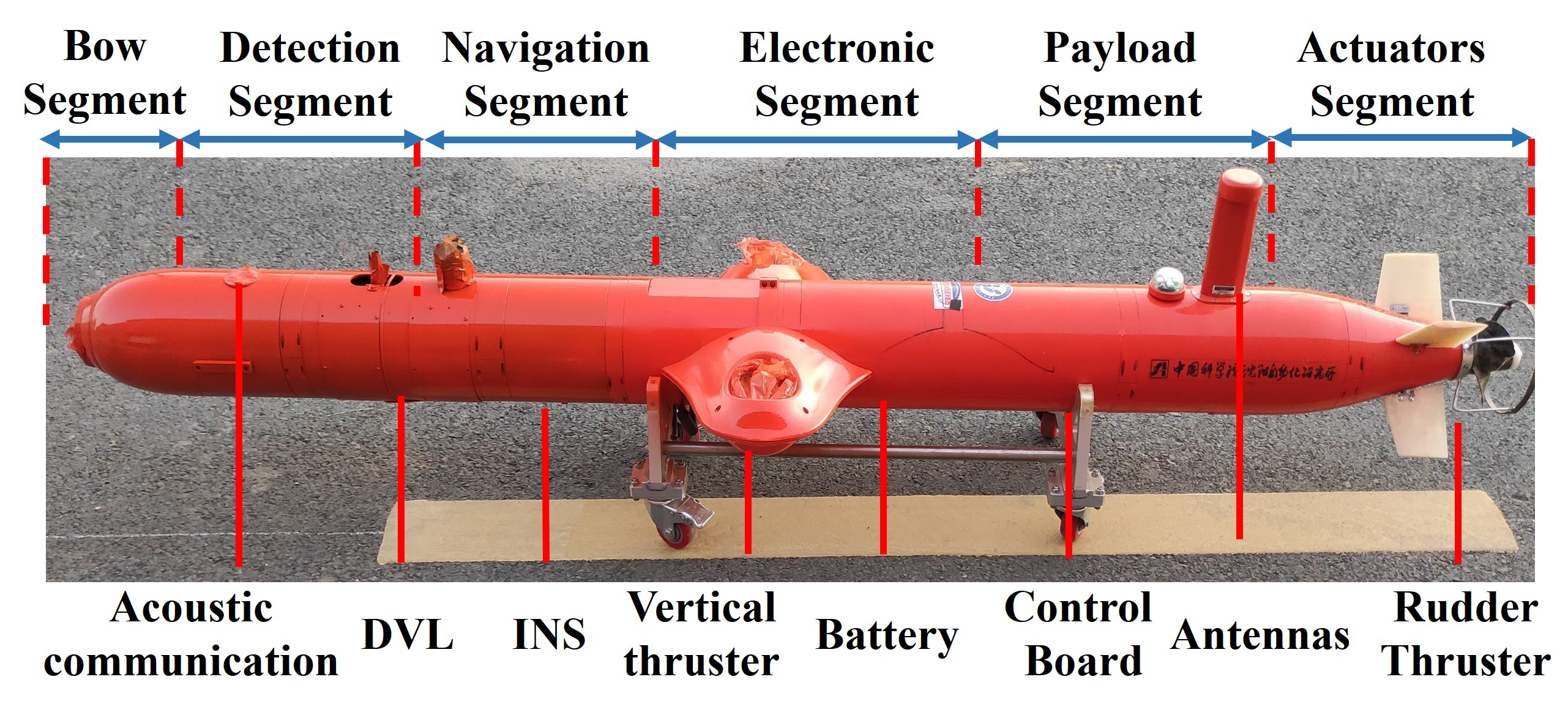
The TS-100 AUV [42] adopts a modular overall architecture. From bow to stern, it consists of the bow segment, detection segment, navigation segment, electronics segment, payload segment, and actuator segment (Figure 9). The detection segment integrates an underwater acoustic communication module, which is used to establish the underwater communication link and support the associated sensing tasks. The navigation segment is equipped with an inertial navigation system (INS), a Doppler velocity log (DVL), and a depth sensor. These subsystems provide attitude and heading information, velocity-aiding measurements, and depth feedback, respectively, thereby supporting underwater dead-reckoning navigation. The electronics segment integrates the battery pack, control board, and an in-hull leak detection unit, supplying electrical power and performing onboard computation and safety monitoring. The payload segment carries antennas that are used for global positioning system (GPS) fixes and Wi-Fi communication when the vehicle is surfaced. The actuator segment incorporates a stern rudder–thruster unit to generate surge thrust and the yaw control moment. In addition, two vertical thrusters are installed near the mid-body of the vehicle; they directly provide heave thrust and differential roll authority, enabling finer depth regulation in the water tank experiments.

4.2. Simulation Result of the TS-100

This subsection reports a numerical simulation of the TS-100 docking-and-seating process under fixed initial conditions and a unified mission script. The simulation uses the same layered guidance/motion controller and the same supervisor/allocation architecture as the later water tank validation. The objective is to isolate the effects of allocation strategy, switching strategy, and fault-tolerant reconfiguration under a common dynamic model and reference command set. The detailed computer configuration is listed in

Table 4. Simulation platform and control periods for the TS-100 numerical study.

Item	Symbol	Value
Host computer CPU	–	AMD Ryzen 7 5800H, 8 cores, 16 threads
Host computer memory	–	15.86 GB RAM
Host operating system	–	Windows 10, 64 bit
Simulation control period	$T_s$	$0.05\mathrm{s}$
TS-100 onboard control frequency	$f_{TS100}$	$25\mathrm{Hz}$
TS-100 onboard control period	$T_{TS100}$	$0.04\mathrm{s}$
Real-time margin criterion	–	Allocator runtime per cycle below $0.04\mathrm{s}$ (onboard) and below $0.05\mathrm{s}$ (simulation)

.

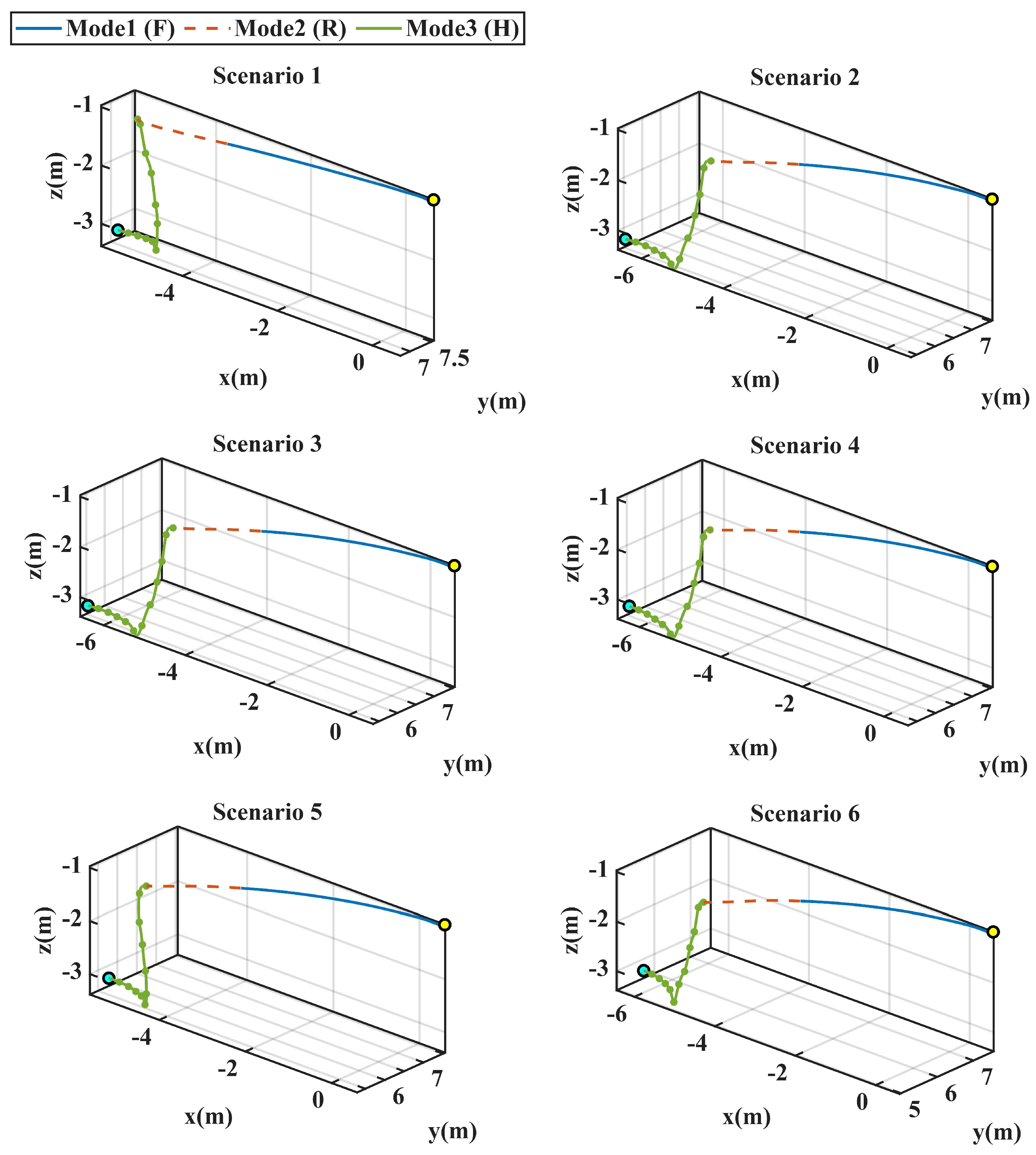
The mission includes three operating modes—forward (F), reverse (R), and hover (H)—with two supervisor-driven transitions (F→R and R→H). Six scenarios are defined in a no-fault set and a fault set. Scenario 1 uses direct PID command generation without control allocation. Scenario 2 uses a weighted least-squares pseudo-inverse allocator as a baseline [7]. Scenarios 3 and 4 use the same multi-mode constrained allocation solver, with hard mode updates in Scenario 3 and bumpless scheduling in Scenario 4. Scenarios 5 and 6 impose identical main propeller effectiveness loss and compare nominal constrained allocation with explicit fault-tolerant allocation. The trajectories for six scenarios are shown in

Table 5. The six simulation scenarios in the TS-100 numerical study.

Scenario	Allocator	Bumpless	FTC	${\mathit{t}}_{\mathit{f}}$ (s)	$\mathit{\alpha }$	Main Objective
S1	PID direct	No	No	–	–	Baseline tracking without CA
S2	WLS pinv	No	No	–	–	Classical CA baseline [7]
S3	MDCA hard	No	No	–	–	MDCA with hard mode update
S4	MDCA bumpless	Yes	No	–	–	Proposed smooth switching
S5	MDCA bumpless	Yes	No	45	0.4	Fault response with nominal CA
S6	MDCA bumpless	Yes	Yes	45	0.4	Fault response with FTC CA

Note: The smooth fault reconstruction duration is $T_{f,sw}=2\mathrm{s}$, and it is applied in Scenario 5 and Scenario 6 only.

.

Figure 10 shows the global trajectories for Scenarios 1–6. All runs complete the same mission sequence, but terminal compactness and post-switching settling differ. In no-fault runs, spread is mainly driven by switching transient quality and redistribution behavior; in fault runs, the trajectory spread primarily reflects the trade-off between feasibility preservation and tracking performance following the loss of control authority. This high-level pattern is supported by state, actuation, wrench, and runtime evidence.

For quantitative evaluation, the controllable wrench tracking error is defined as

$$e_{\tau }={\mathit{\tau }}_d-{\mathit{\tau }}_c,$$

(66)

and the switching jump indices are defined as

$$d{u}_{\infty ,\mathrm{FR}}=\underset{k\in {\mathcal{W}}_{FR}}{\max }{\parallel \Delta \mathit{u}\left(k\right)\parallel }_{\infty },d{u}_{\infty ,\mathrm{RH}}=\underset{k\in {\mathcal{W}}_{RH}}{\max }{\parallel \Delta \mathit{u}\left(k\right)\parallel }_{\infty },$$

(67)

where $\Delta \mathit{u}\left(k\right)=\mathit{u}\left(k\right)-\mathit{u}(k-1)$, and ${\mathcal{W}}_{FR}$ and ${\mathcal{W}}_{RH}$ are fixed windows around the two switching instants. In the no-fault group, the extracted switching times are $t_{FR}=24\mathrm{s}$ for all four scenarios, while $t_{RH}=40.15\mathrm{s}$ in Scenario 1 and $t_{RH}=46\mathrm{s}$ in Scenarios 2–4. These indices are evaluated together with the saturation ratio to quantify tracking quality, switching smoothness, and the feasibility margin.

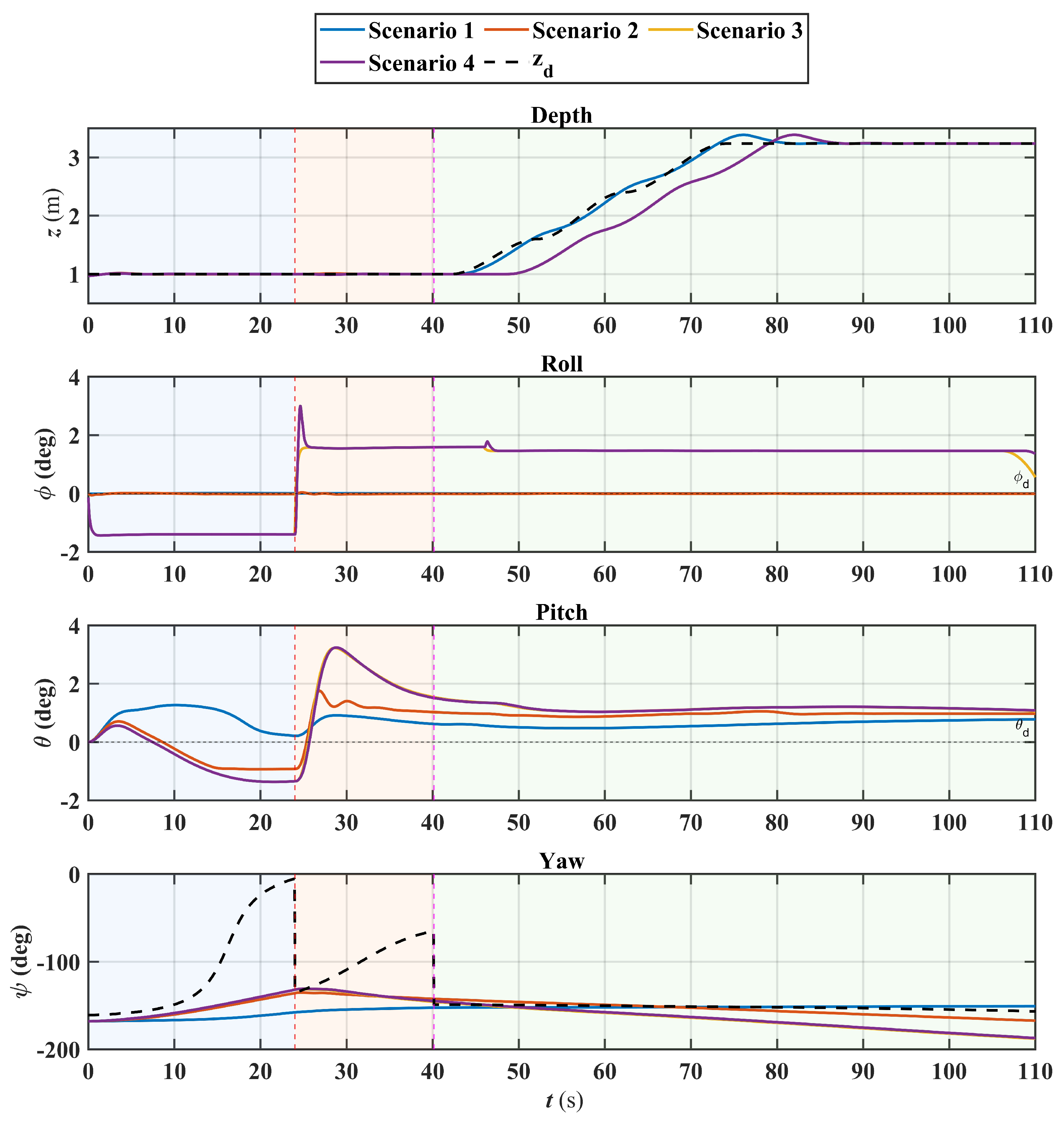
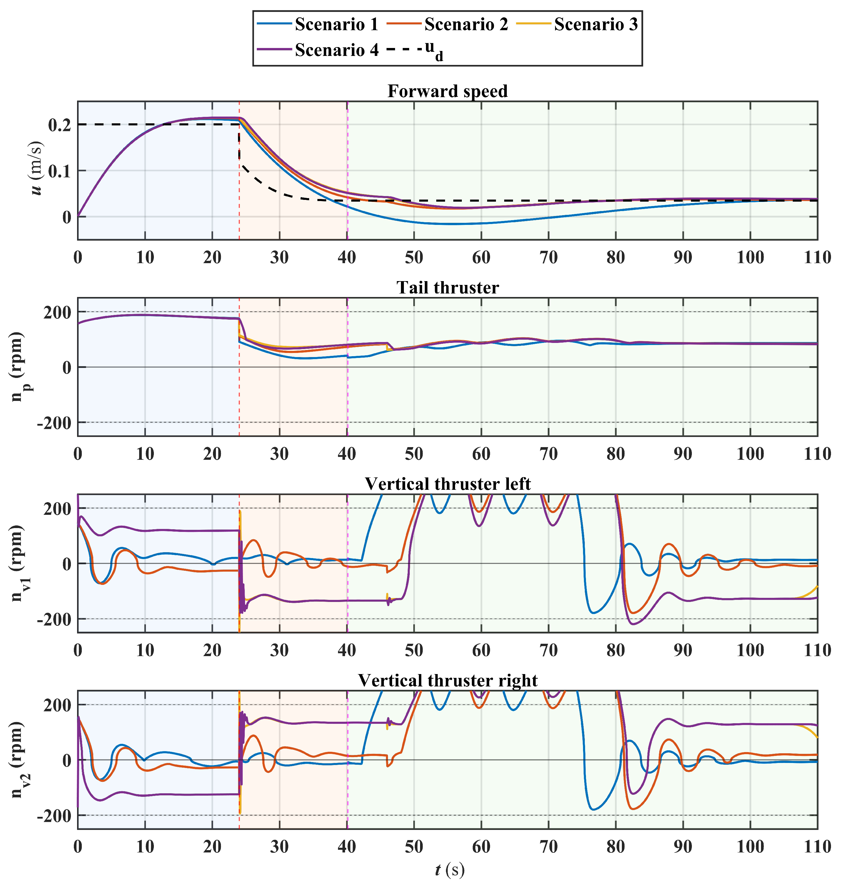
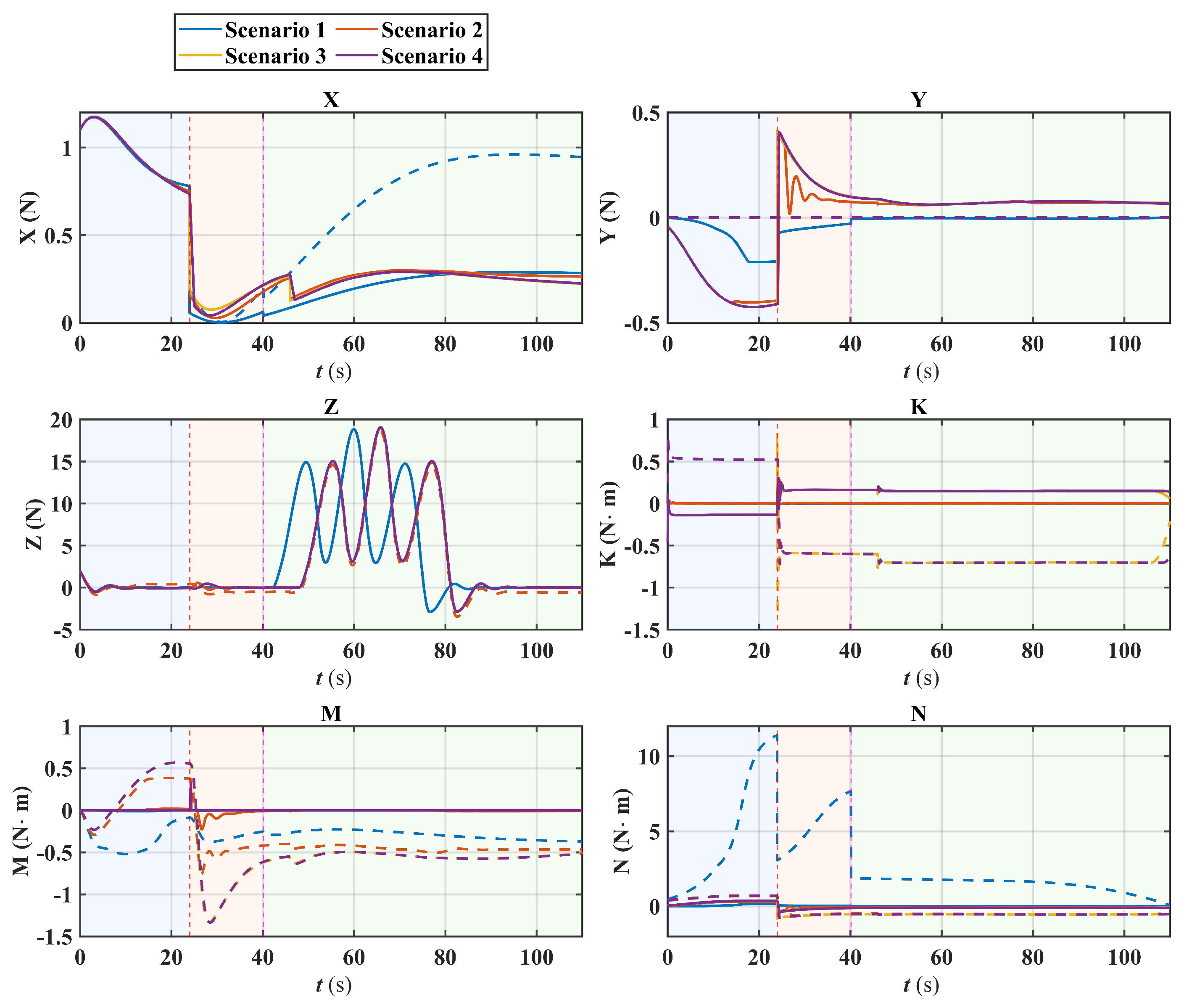
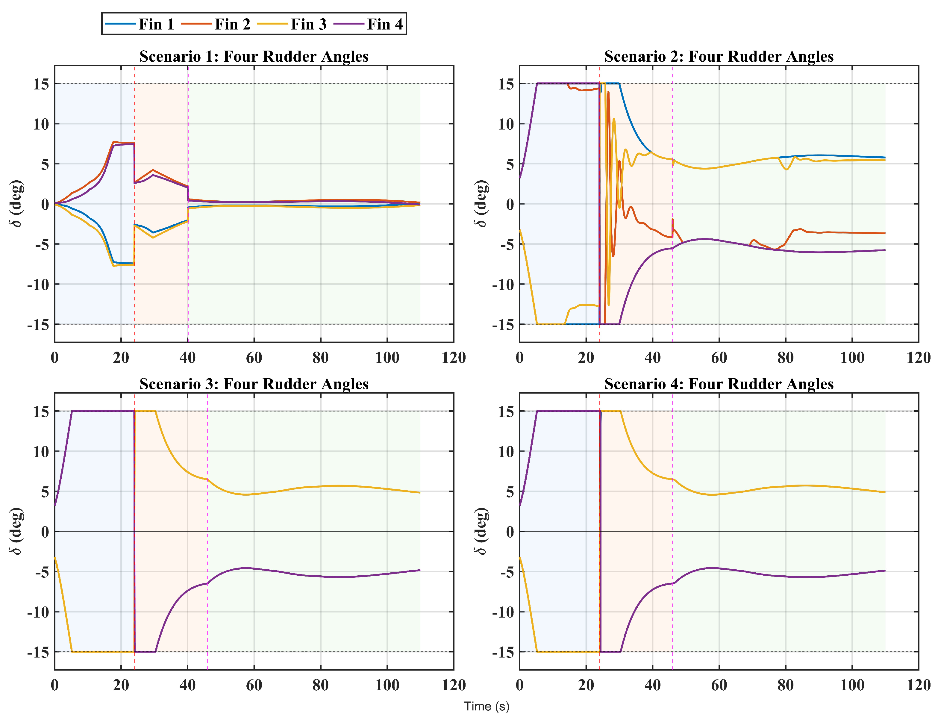
The no-fault comparison in Figure 11, Figure 12 and Figure 13, Figure 14, and

Table 6. No-fault comparison metrics for Scenarios 1 to 4.

Scenario	$\mathbf{RMS}\left({\mathit{e}}_{\mathit{\tau },\mathbf{all}}\right)$	${\mathit{r}}_{\mathbf{sat},\mathbf{all}}$	${\mathit{du}}_{\mathit{\infty },\mathbf{FR}}$	${\mathit{du}}_{\mathit{\infty },\mathbf{RH}}$
S1	3.7978	0.0000	0.7248	0.0209
S2	0.7836	0.9995	0.5817	0.1212
S3	1.0686	0.9991	4.8027	0.2611
S4	1.0719	1.0000	0.9044	0.0978

yields three quantitative findings: $\mathrm{RMS}\left(e_{\tau ,\mathrm{all}}\right)$ decreases from 3.7978 to 1.0719 (71.78%), $d{u}_{\infty ,\mathrm{FR}}$ decreases from 4.8027 to 0.9044 (81.17%), and $d{u}_{\infty ,\mathrm{RH}}$ decreases from 0.2611 to 0.0978 (62.53%).

Under external loads and the model mismatch represented by ${\mathit{\tau }}_e$, this behavior indicates that the closed-loop system absorbs uncertainty through coordinated multi-actuator feedback and avoids abrupt single-channel takeover during mode transitions.

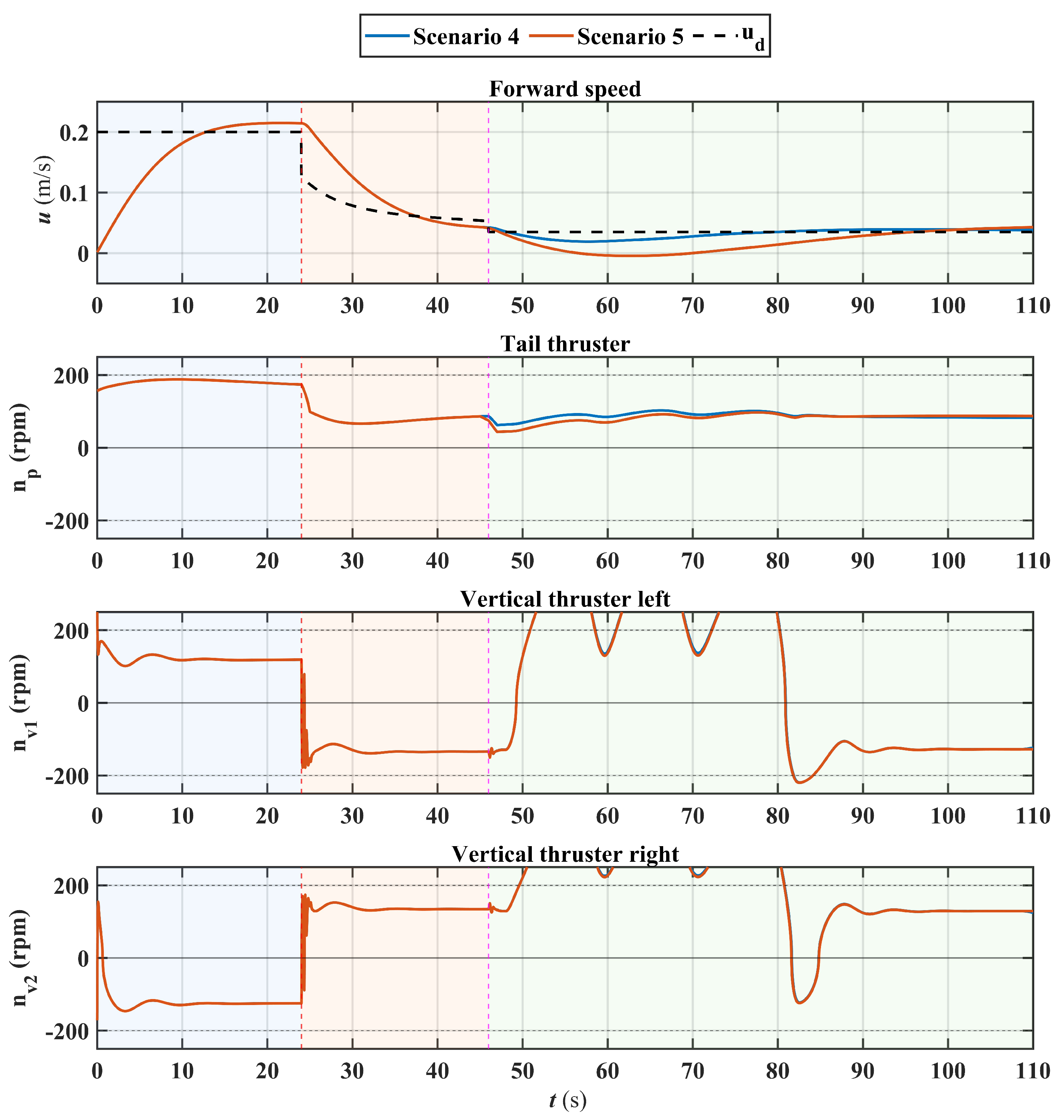
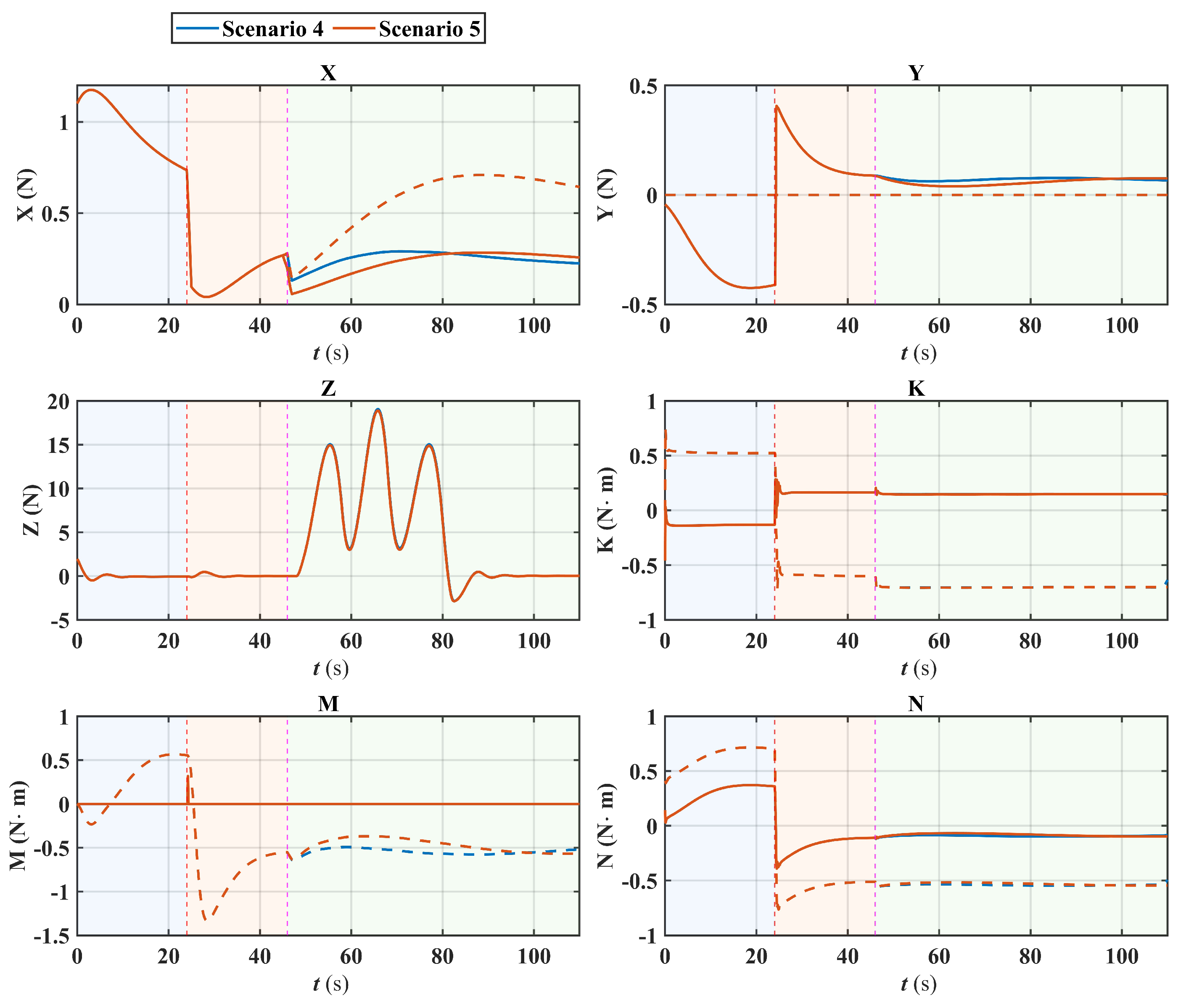
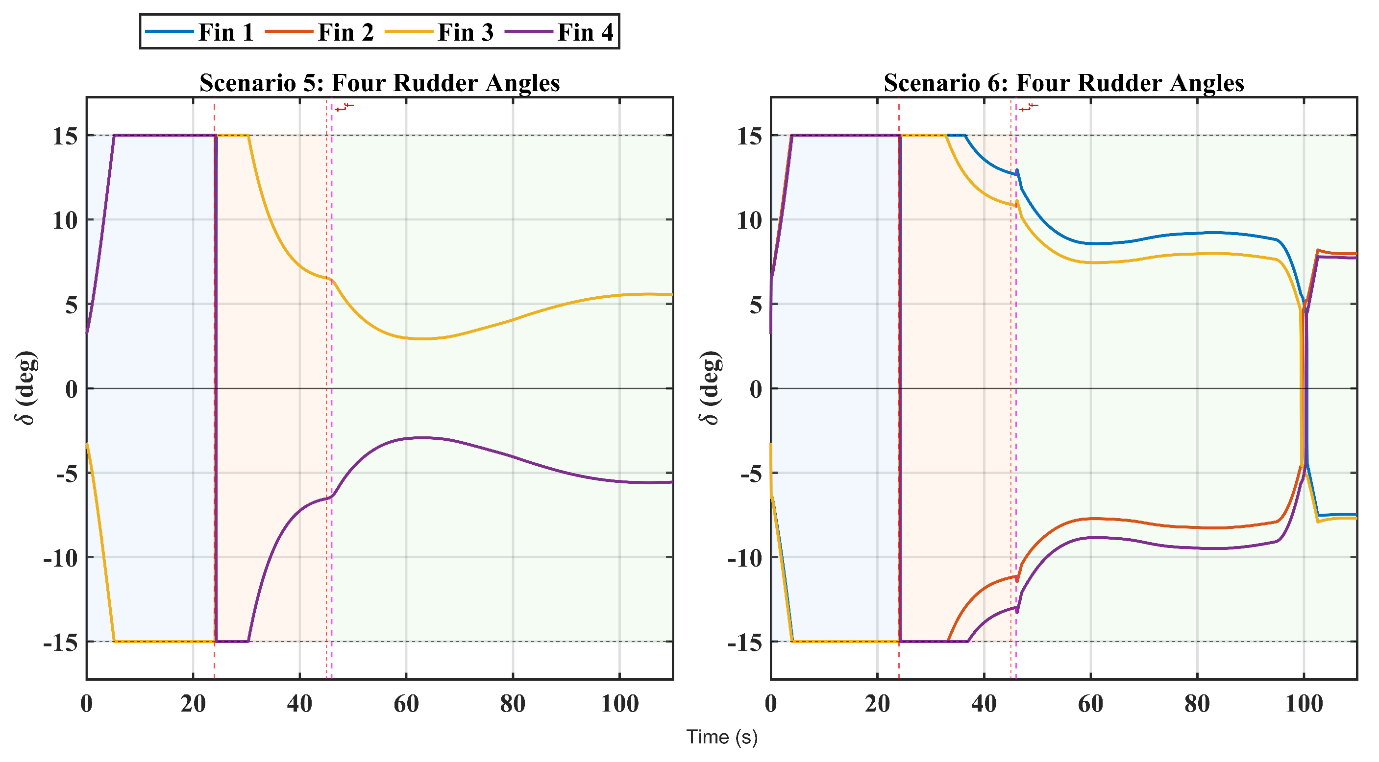
Fault-tolerance behavior is summarized in

Table 7. Fault-tolerant metrics for Scenarios 5 and 6.

Scenario	Strategy	$\mathbf{RMS}\left({\mathit{e}}_{\mathit{\tau },\mathbf{post}}\right)$	$\mathit{d}{\mathit{\theta }}_{\mathbf{fault}}$	$\mathit{d}{\mathit{\psi }}_{\mathbf{fault}}$	${\mathit{s}}_{\max }$	${\mathit{s}}_{\mathbf{RMS}}$
S5	Nominal CA	1.1335	0.02870	1.4397	N.A.	N.A.
S6	FTC CA	0.9988	0.02607	2.1170	0.01976	0.02343

and Figure 15, Figure 16 and Figure 17. After main propeller degradation at $t_f=45\mathrm{s}$, Scenario 6 improves key post-fault indices relative to Scenario 5. The post-fault wrench error decreases from 1.1335 to 0.9988 (11.88%), and the pitch-related deviation index decreases from 0.02870 to 0.02607 (9.16%).

The trace-level evidence clarifies the mechanism. After fault onset, thrust and rudder commands in Scenario 6 are redistributed more systematically across remaining channels, while the realized wrench remains structured during recovery. This reflects priority-based reallocation under reduced authority.

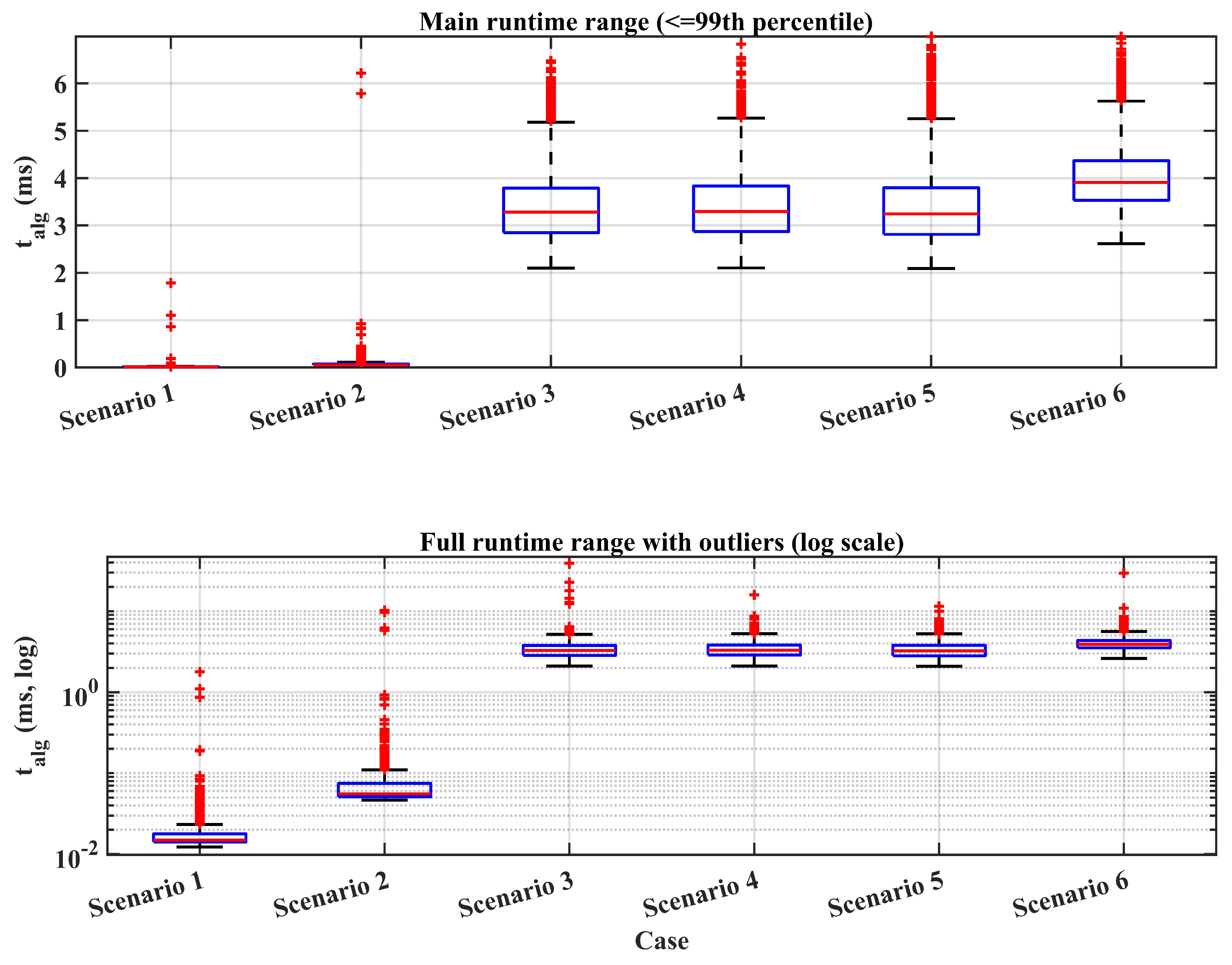
Runtime performance is reported in

Table 8. Allocator runtime statistics for the six scenarios in milliseconds per control cycle.

Scenario	Mean	Std	p95	Max
S1	0.0192	0.0484	0.0293	1.7855
S2	0.0887	0.4123	0.1254	10.2996
S3	3.4195	1.2371	4.8314	39.3173
S4	3.4190	0.8293	4.8913	15.8738
S5	3.4183	0.9007	5.2526	11.5384
S6	4.0502	0.9748	5.5163	29.5856

and Figure 18. In degraded operation, Scenario 6 increases mean runtime from 3.4183 to 4.0502 ms relative to Scenario 5 (18.49%) because of fault-aware processing and soft-constraint handling.

Despite this increase, real-time feasibility remains clear. The maximum runtime in Scenario 6 is 29.5856 ms, below both the TS-100 onboard period (40 ms) and the simulation period (50 ms). The p95 runtime is 5.5163 ms, leaving a large cycle margin.

Overall, the simulation results establish a consistent evidence chain for the subsequent experimental section. In no-fault operation, bumpless multi-mode allocation improves transition smoothness while preserving tracking performance. In fault operation, the fault-tolerant extension improves key post-fault indices with controlled relaxation and an explicit yaw tradeoff.

4.3. Tank Scenarios of the TS-100

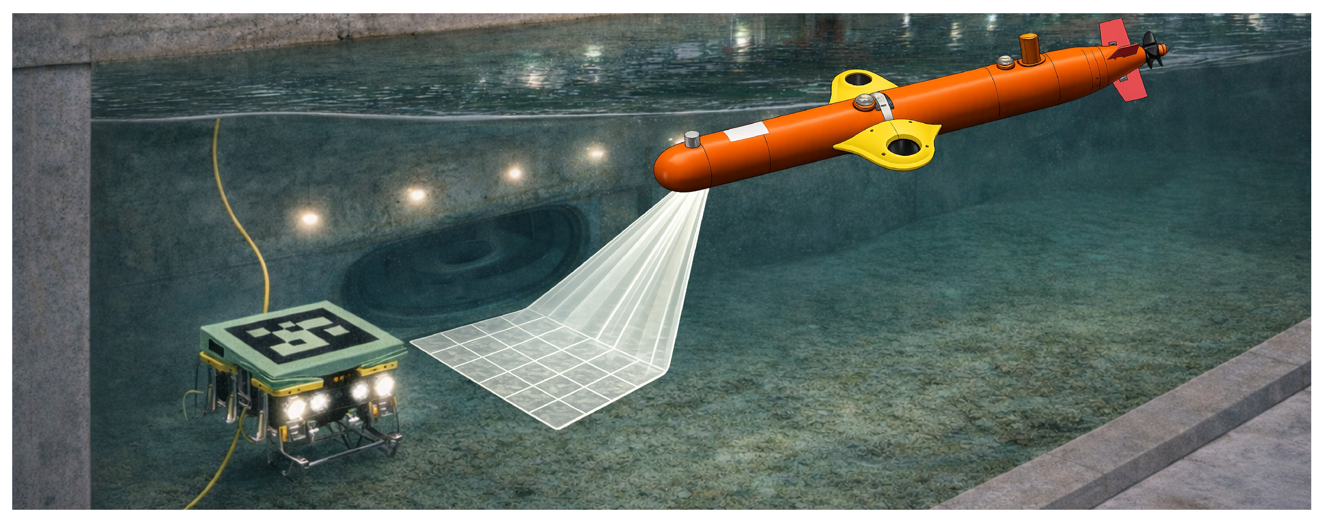
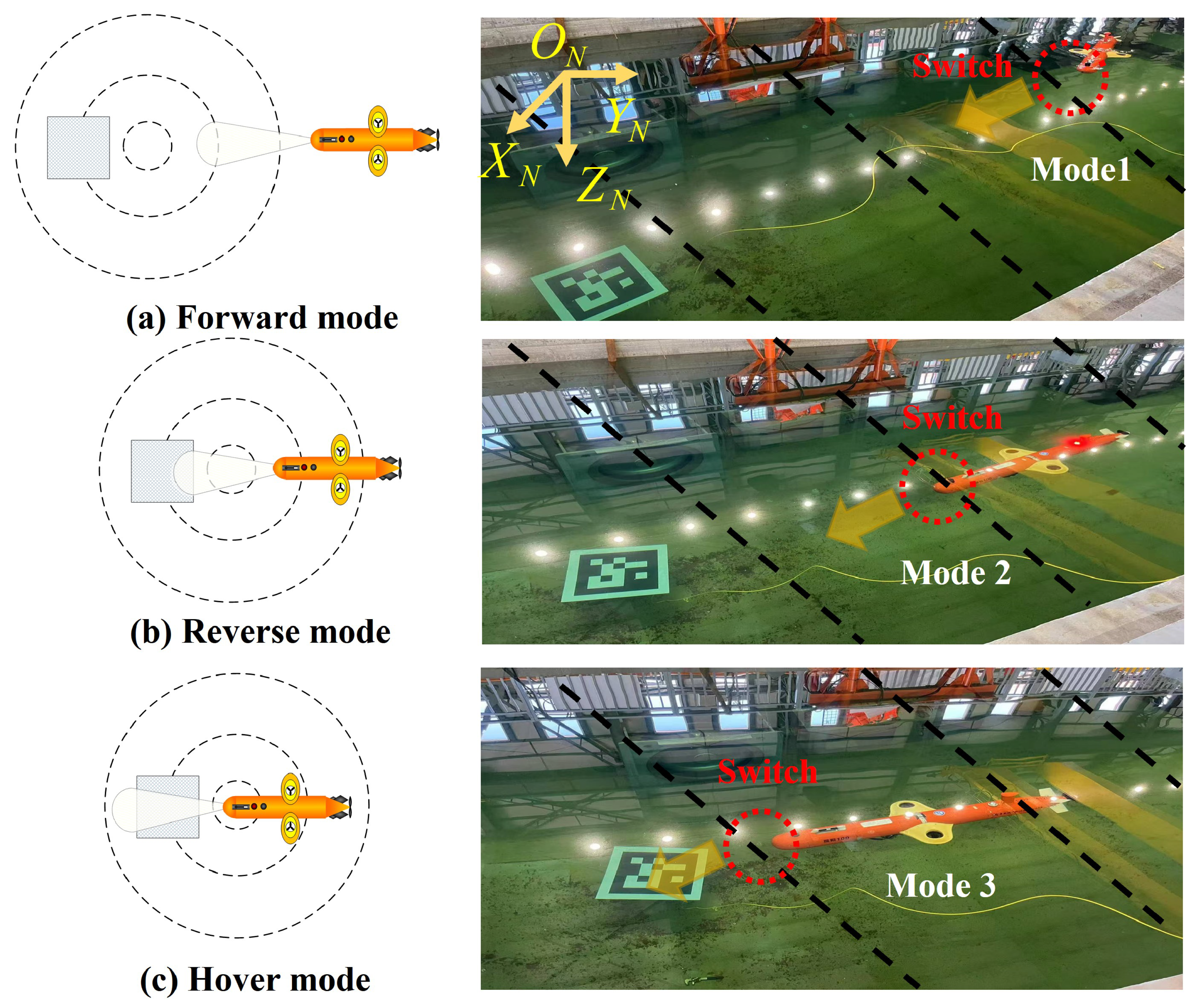
Water tank experiments were conducted in a $60\mathrm{m}\times 100\mathrm{m}$ water tank environment, with QR codes serving as visual observation targets, as shown in Figure 19. The TS-100 AUV executed a three-phase mission. It first tracked a predefined straight-line trajectory, as shown in Figure 20a.

In the tank tests, the detection flag ${\chi }_k$ was produced by the onboard QR-code recognition module, and the range variable $d_k$ in (53) was obtained by stereo camera.

To evaluate the effects of CA and bumpless switching in the same mission, three comparative scenarios were designed under identical initial conditions with the same initial distance to the target and the same mission procedure. In all three scenarios, the guidance (ALOS) and motion-control (PID) layers were identical; the comparison isolated the effects of (i) constrained control allocation (CA) and (ii) bumpless mode switching.

(1) Scenario 1: PID baseline (no CA, hard switching). The vehicle cruised along a predefined baseline trajectory. Once the onboard camera detected the QR code, the stern thruster command was set to zero. The vehicle then decelerated by coasting under hydrodynamic damping. After arriving above the target, it switched directly to hovering control, and the attitude was regulated using the vertical thrusters. A hard switch was adopted for mode transition.

(2) Scenario 2: CA only, without bumpless switching. An SQP-based CA framework was enabled. The vehicle cruised along the predefined baseline trajectory, and the desired forces and moments were allocated online during the deceleration and hovering phases. During mode switching, bumpless switching was not applied, and no transitional scheduling or state alignment was performed. Consequently, the CA parameter matrix was updated abruptly at the switching instant, and the outer-loop integral states were not aligned.

(3) Scenario 3: CA with bumpless switching. The complete framework proposed in this paper was enabled, in which bumpless switching was integrated into multi-mode CA. A continuous transition factor was used to smoothly schedule the CA weight matrix, and the outer-loop integral states for depth and heading were aligned at the switching instant, thereby suppressing command discontinuities and transient shocks induced by mode switching.

4.4. Multi-Mode Switching Experiments

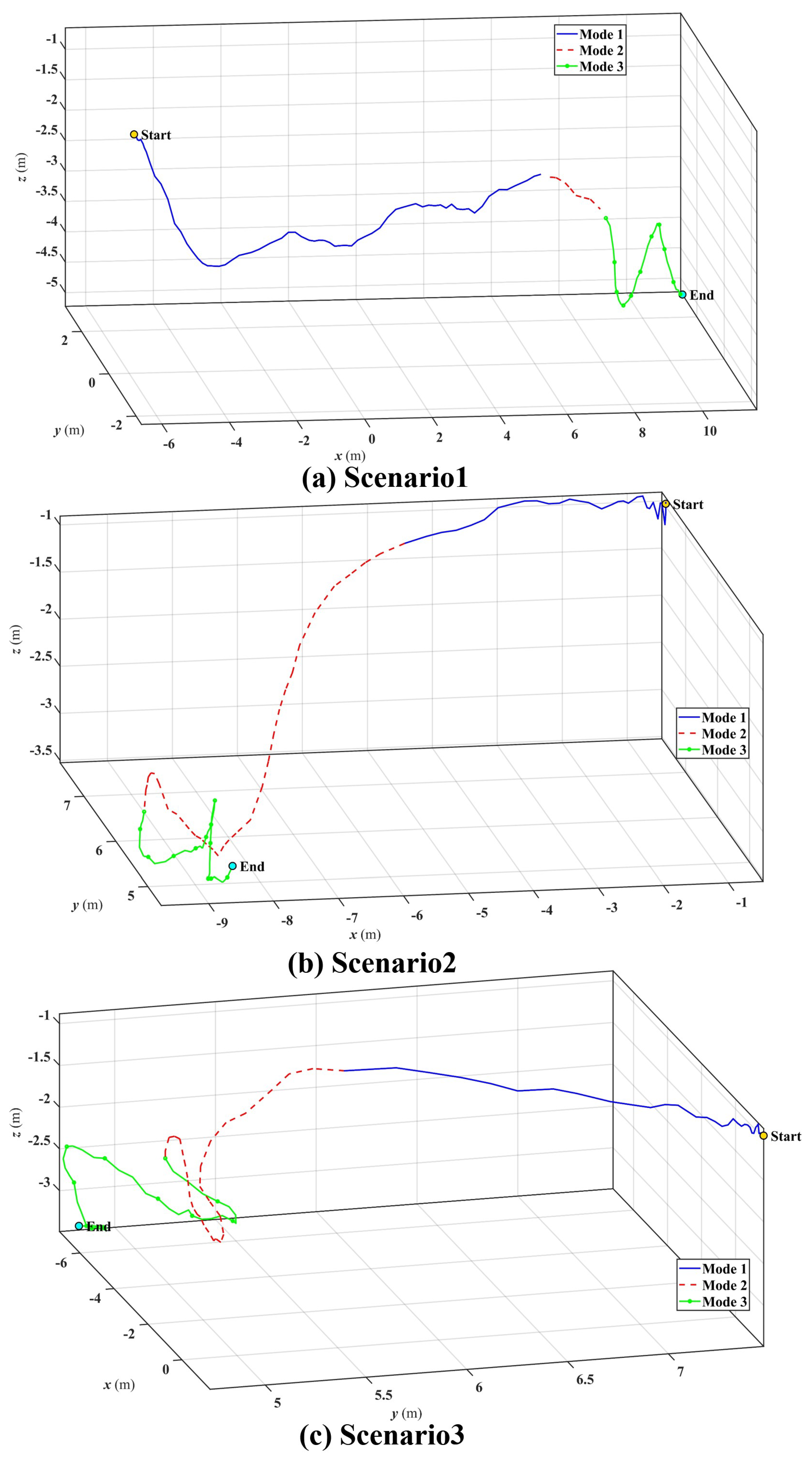
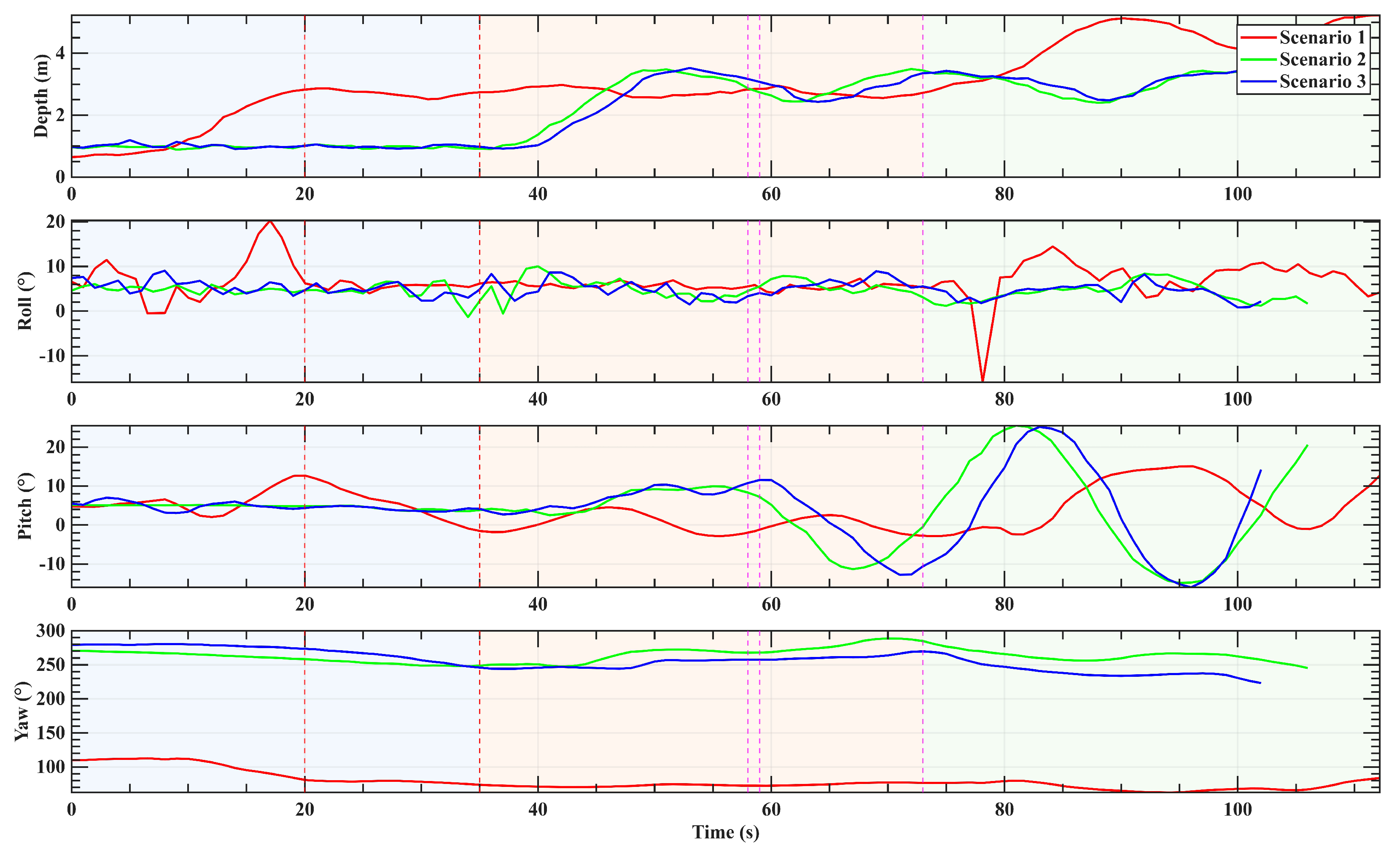
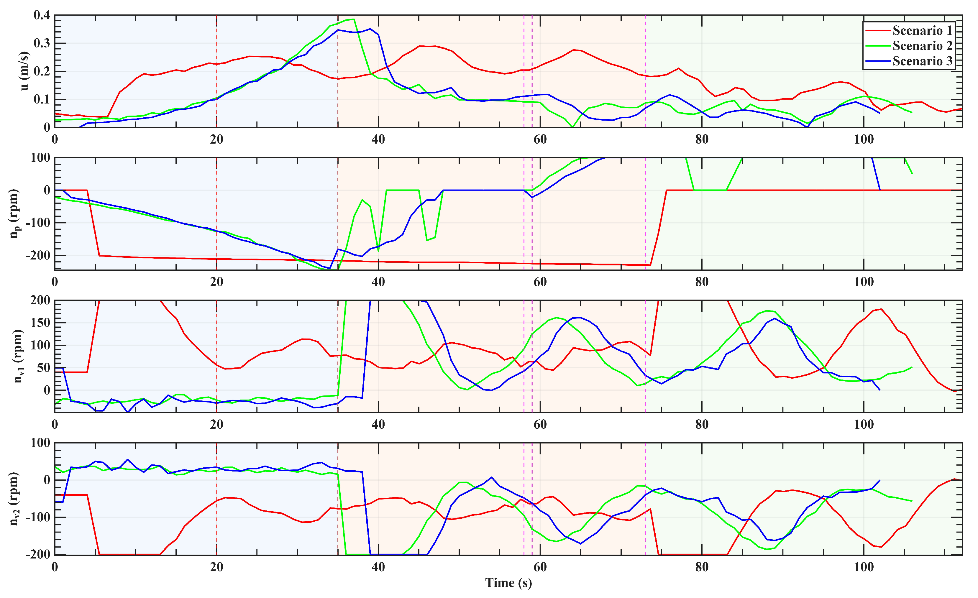
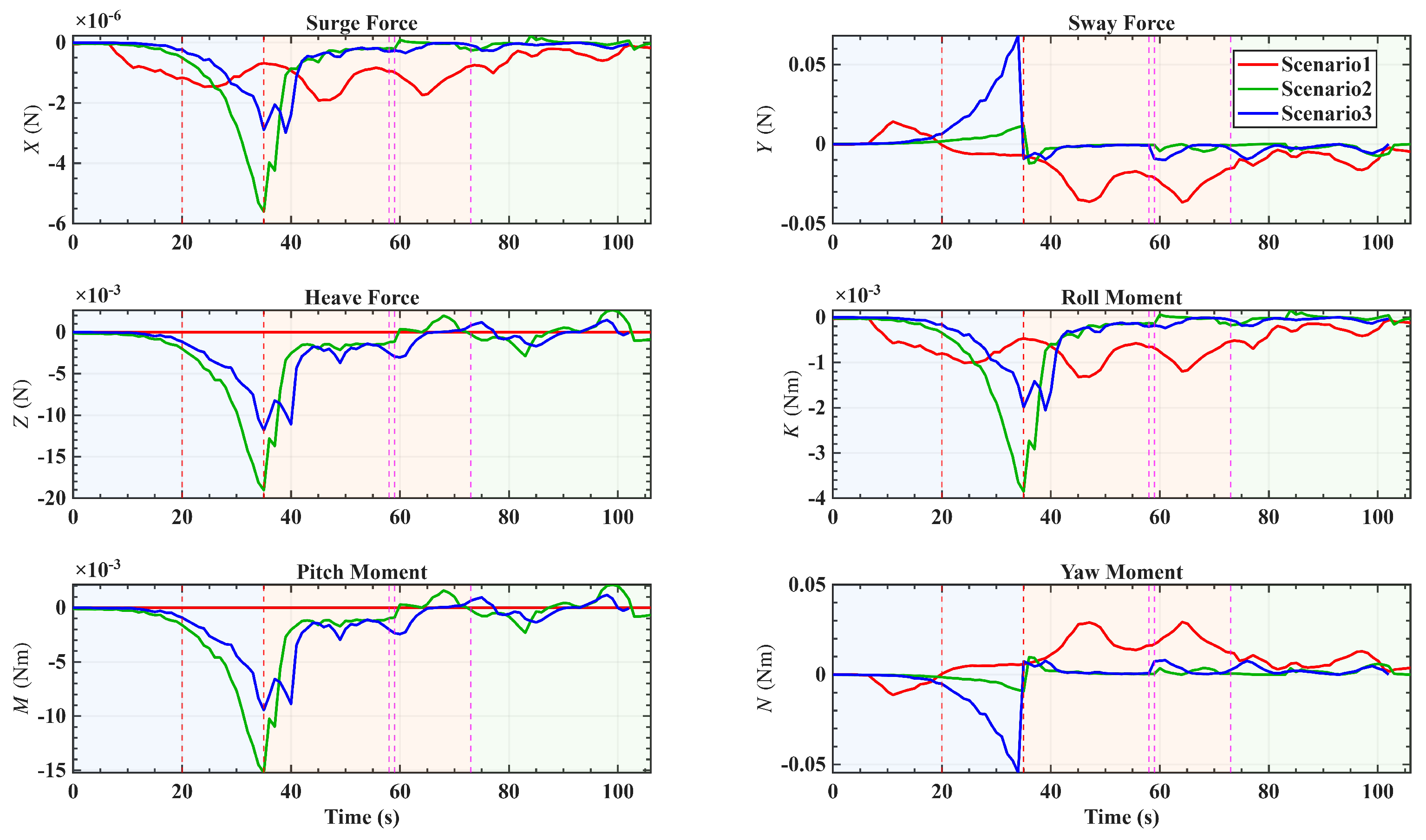
To evaluate multi-mode switching transients in the tank experiments, the three comparative scenarios were analyzed using a unified post-processing rule. The extracted switching times are Scenario 1 ($t_{FR}=70\mathrm{s}$, $t_{RH}=80\mathrm{s}$), Scenario 2 ($t_{FR}=37\mathrm{s}$, $t_{RH}=65\mathrm{s}$), and Scenario 3 ($t_{FR}=36\mathrm{s}$, $t_{RH}=68\mathrm{s}$).

Figure 21 shows that all three runs completed the forward, deceleration, and hover sequence, yet the terminal behavior in Mode H differed. In Scenario 1, the vehicle exhibits larger residual oscillation and drift near the target, with continuous position and attitude corrections, indicating weaker station keeping when CA is not used and mode switching is hard. With CA enabled in Scenario 2 and Scenario 3, the terminal trajectory becomes more concentrated, suggesting improved actuator coordination under constraints. Scenario 3 achieves the smallest terminal drift in Mode H, consistent with the intended multi-mode coordination and smoother switching behavior.

The depth and attitude responses in Figure 22 reveal the switching behavior and the subsequent hover stability. Scenario 1 shows the largest roll fluctuation in the hover segment, where the Roll RMS in Mode H reaches 4.707 deg (

Table A5. Hover-mode stability and switching-window transients using multi-mode segmentation. FR max. step and RH max. step are computed as the maximum adjacent-sample step within a $2\mathrm{s}$ half-width window centered at $t_{FR}$ and $t_{RH}$.

Scenario	Hover Mode H						FR Max. Step			RH Max. Step
	Depth RMS	Depth P2P	Roll RMS	Pitch RMS	Yaw RMS	$\mathit{u}$ Mean	${\mathit{n}}_{\mathit{p}}$	$\Delta$	Roll	${\mathit{n}}_{\mathit{p}}$	$\Delta$	Roll
	$\mathbf{m}$	$\mathbf{m}$	$\mathbf{deg}$	$\mathbf{deg}$	$\mathbf{deg}$	$\mathbf{m}/\mathbf{s}$	$\mathbf{rpm}$	$\mathbf{deg}$	$\mathbf{deg}$	$\mathbf{rpm}$	$\mathbf{deg}$	$\mathbf{deg}$
S1	0.735	2.458	4.707	6.442	6.201	0.119	1.000	0.652	6.259	99.000	1.653	1.353
S2	0.351	1.090	2.008	12.644	10.651	0.068	100.000	2.377	6.114	25.000	6.820	1.653
S3	0.318	0.998	1.838	12.416	13.323	0.063	59.000	7.408	3.496	22.000	6.593	1.431

). In the RH switching window, the roll max. step values are 1.353 deg, 1.653 deg, and 1.431 deg for Scenarios 1–3, respectively. With CA only, Scenario 2 reduces the hover-mode Roll RMS to 2.008 deg, indicating that constrained allocation mitigates the low-speed attitude fluctuation. With CA plus bumpless switching, Scenario 3 further reduces the hover-mode Roll RMS to 1.838 deg. For the hover segment H, Table A5 shows a consistent improvement of depth station keeping across the two upgrades, where Depth RMS decreases from 0.735 m in Scenario 1 to 0.351 m in Scenario 2 and further to 0.318 m in Scenario 3, and Depth P2P decreases from 2.458 m to 1.090 m and further to 0.998 m. Meanwhile, the hover mean speed decreases from 0.119 m/s to 0.068 m/s and further to 0.063 m/s, indicating progressively tighter station keeping in Mode H.

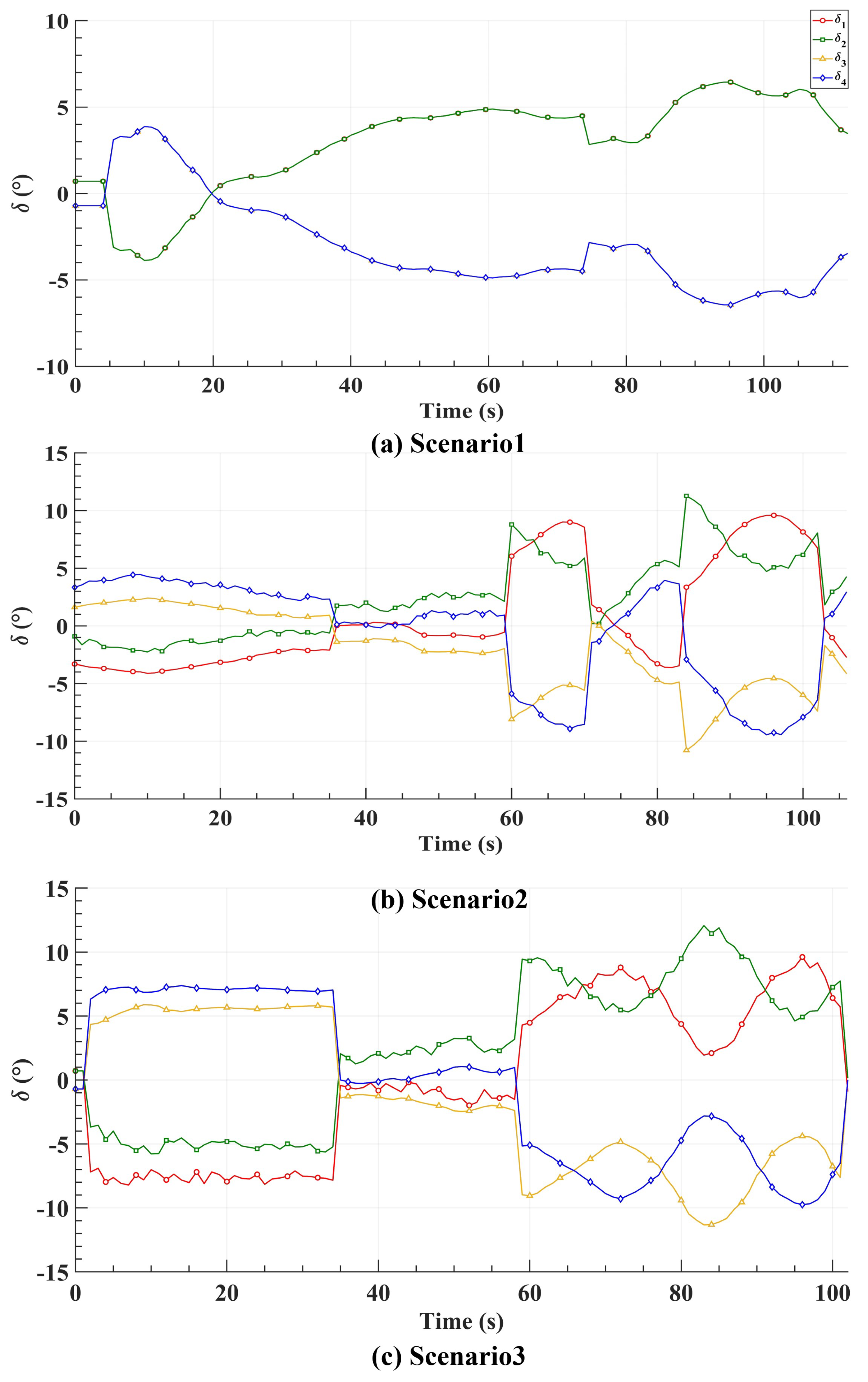
The actuation-side evidence is provided by Figure 23 and Figure 24. Scenario 1 applies a hard propulsion strategy in the deceleration and hover phases. Around $t_{FR}$, Table A5 shows that Scenario 2 exhibits a stronger thruster command step, with an FR $n_p$ max. step of 100 rpm, whereas Scenario 3 reduces it to 59 rpm. In contrast, the fin command step around $t_{FR}$ increases when moving from Scenario 2 to Scenario 3, where the FR $\Delta$ max. step rises from 2.377 deg to 7.408 deg. Together with the per-mode actuation RMS values in

Table A6. Full per-mode performance metrics using phaseEdges segmentation.

Scenario	Mode	Duration $\mathbf{s}$	N	State Metrics						Actuation RMS
				Depth RMS $\mathbf{m}$	Depth P2P $\mathbf{m}$	Roll RMS $\mathbf{deg}$	Pitch RMS $\mathbf{deg}$	Yaw RMS $\mathbf{deg}$	$\mathit{u}$ Mean $\mathbf{m}/\mathbf{s}$	${\mathit{n}}_{\mathit{p}}$ RMS $\mathbf{rpm}$	${\mathit{n}}_{\mathit{v}\mathbf{1}}$ RMS $\mathbf{rpm}$	${\mathit{n}}_{\mathit{v}\mathbf{2}}$ RMS $\mathbf{rpm}$	$\Delta$ RMS $\mathbf{deg}$
S1	F	19.032	19	0.767	2.136	5.484	2.747	9.432	0.135	177.644	149.247	149.247	2.485
S1	R	52.085	49	0.123	0.466	0.707	3.880	2.950	0.227	220.455	79.598	79.598	3.678
S1	H	38.563	38	0.735	2.458	4.707	6.442	6.201	0.119	42.938	126.473	126.473	5.090
S2	F	34.000	35	0.038	0.174	1.436	0.518	7.471	0.119	134.577	22.641	27.520	3.510
S2	R	23.000	24	0.939	2.574	2.367	2.770	9.868	0.161	87.067	130.895	132.392	2.221
S2	H	47.000	48	0.351	1.090	2.008	12.644	10.651	0.068	88.059	96.537	101.059	7.362
S3	F	34.000	35	0.061	0.286	1.552	0.997	9.749	0.108	132.161	30.879	35.717	7.399
S3	R	22.000	23	1.010	2.605	2.043	2.524	5.348	0.181	112.164	126.673	128.213	2.374
S3	H	44.000	45	0.318	0.998	1.838	12.416	13.323	0.063	89.882	90.950	94.506	8.981

, this indicates a redistribution of short-horizon control effort from thrusters toward fins during the transition, while the overall hover stability continues to improve. This redistribution is consistent with multi-mode CA under bumpless scheduling, where the allocation weights and internal states evolve more continuously, thereby avoiding abrupt solution jumps in the dominant actuation channels.

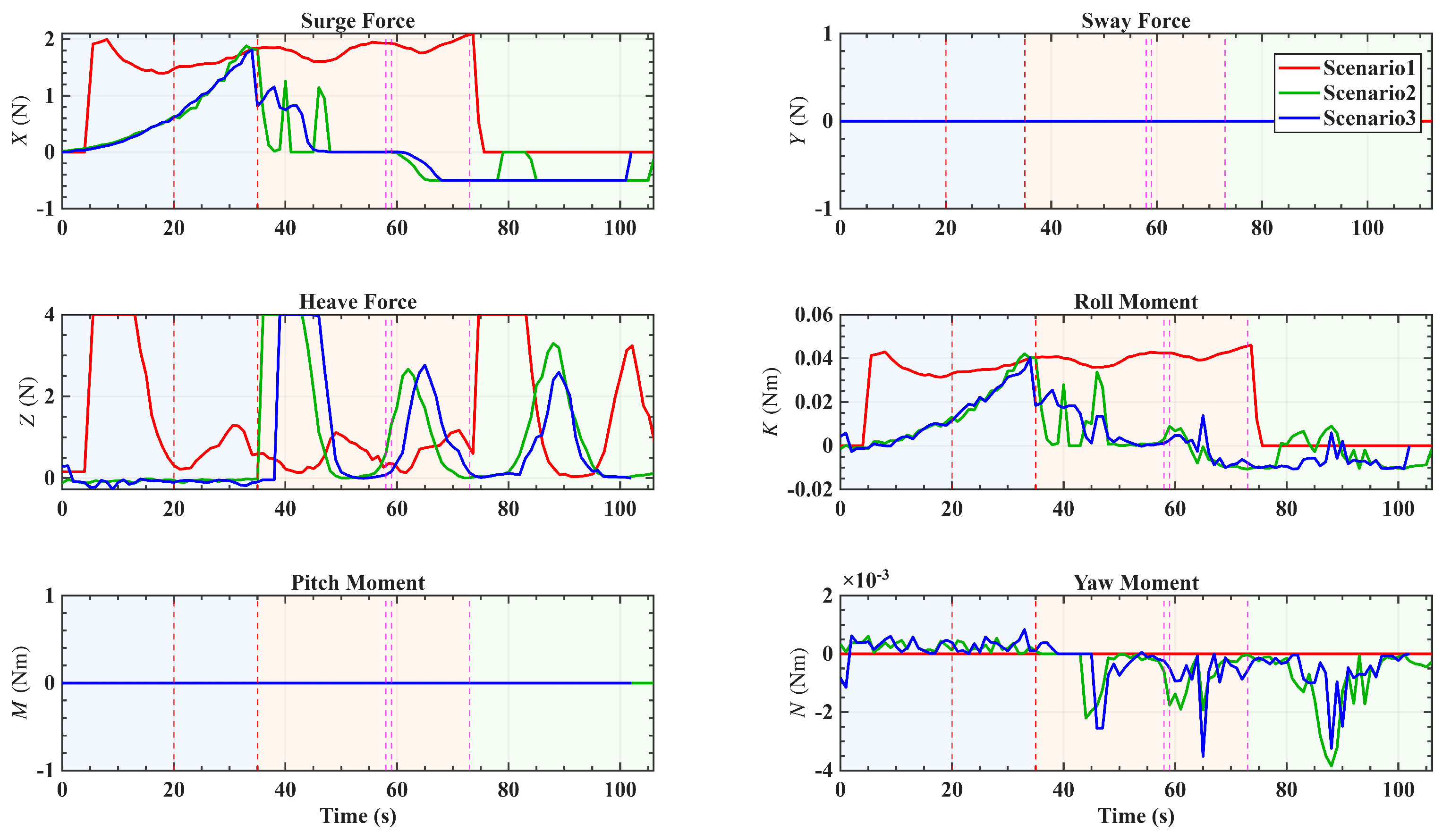
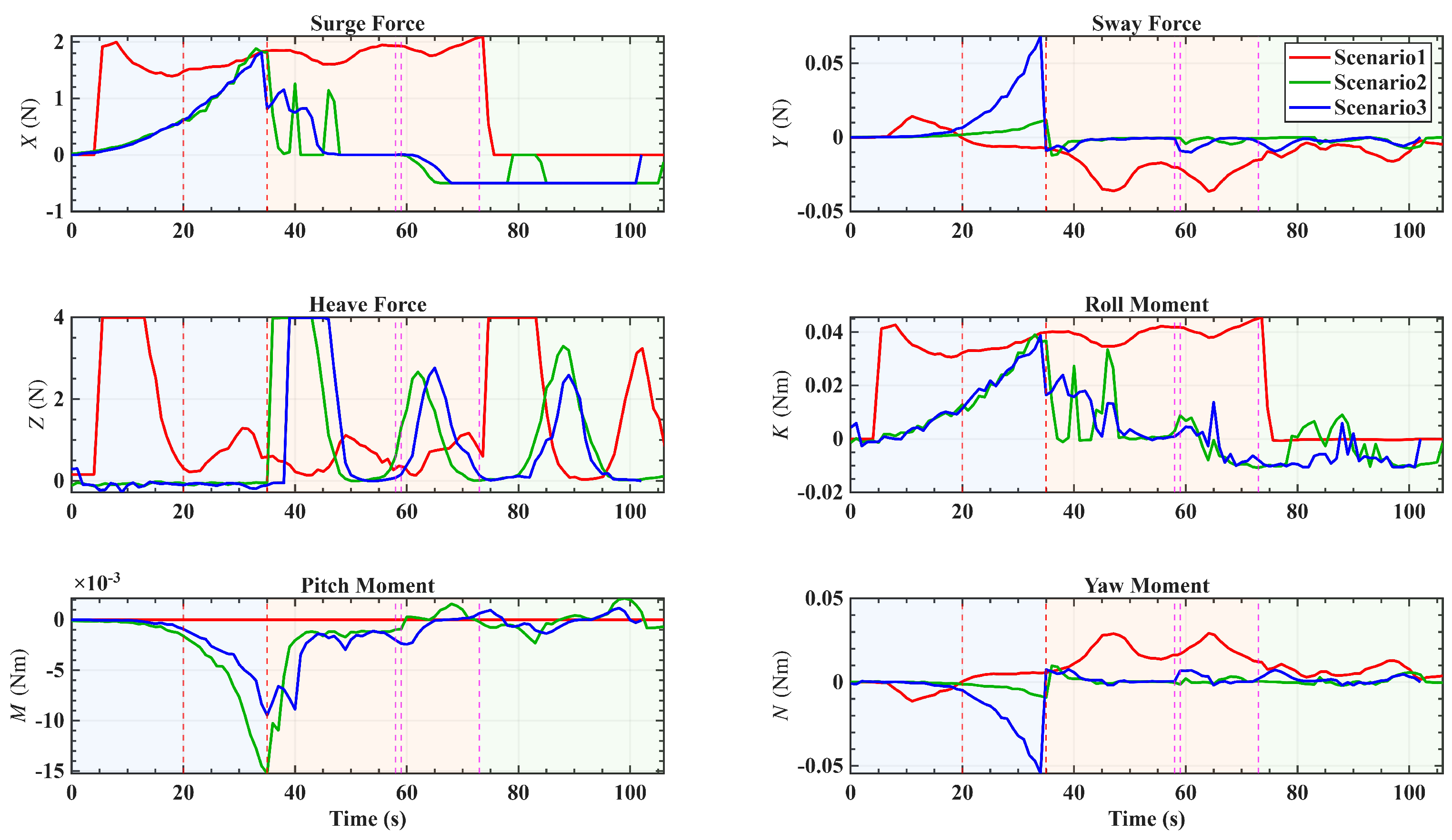
The wrench decomposition in Figure 25, Figure 26 and Figure 27 further supports the above interpretation. With CA enabled, the demanded wrench is not borne by a single actuator group, and both fins and thrusters contribute across modes. The total actuator wrench exhibits a more structured evolution during switching in Scenario 2 and Scenario 3 than in Scenario 1, which reduces the likelihood of abrupt saturation and impact-like transients.

5. Discussion

Overall, the tank results support the intended separation of benefits: CA improves feasibility and coordination (Scenario 2 vs. Scenario 1), and bumpless switching further improves switching behavior and hover depth station keeping (Scenario 3 vs. Scenario 2).

Several limitations remain: The allocator depends on effectiveness and constraint models that vary with speed and flow conditions, so robustness to model mismatch, unmodeled actuator dynamics, and environmental disturbances (e.g., currents) should be strengthened. Future work should include open-water validation with contact-relevant docking dynamics and fault/saturation scenarios.

6. Conclusions

This paper presents a bumpless multi-mode control allocation framework for over-actuated AUV docking across forward cruise, reverse approach, and hover observation. The MD-CA formulation unifies mode supervision and constrained allocation within one SQP structure while scheduling objectives and constraints by mode. Allocation targets controllable wrench components X, Z, K, M, and N under amplitude and increment limits. Bumpless switching is achieved by transition factor scheduling, PID integrator alignment, and warm-starting via feasibility projection.

The framework was integrated into MOOS-IvP with ALOS guidance and validated on TS-100 water tank experiments. Compared with no-CA and CA-only baselines, the proposed method improves actuator coordination under constraints and reduces switching-induced attitude disturbances, especially near reverse-to-hover transition.

Current validation is limited to a controlled tank environment, a three-mode procedure, and one vehicle configuration. Future work will broaden operating conditions, improve systematic tuning of mode-scheduled parameters, and strengthen robustness to target loss and modeling errors.

References

1. Li, C.; Guo, S. Adaptive Multi-Mode Switching Strategy for the Spherical Underwater Robot with Hybrid Thrusters. Adv. Eng. Inform. 2023, 55, 101845. [Google Scholar] [CrossRef]
2. Huang, Y.; Li, Y.; Yu, J.; Li, S.; Feng, X. State-of-the-art and development trends of AUV intelligence. Robot 2020, 42, 215–231. [Google Scholar] [CrossRef]
3. Fu, J.; Zhou, H.; Wu, W.; Zhang, X.; Yao, B.; Lian, L.; Mao, Z. A Novel In-Situ Heading Control Strategy for the Multi-Mode Underwater Vehicle. Ocean. Eng. 2025, 322, 120529. [Google Scholar] [CrossRef]
4. Walmsness, J.E.; Helgesen, H.H.; Larsen, S.; Kufoalor, G.K.M.; Johansen, T.A. Automatic dock-to-dock control system for surface vessels using bumpless transfer. Ocean. Eng. 2023, 268, 113425. [Google Scholar] [CrossRef]
5. Li, J.; Zhao, J. Bumpless transfer control for switched linear systems with bump induced event-triggered mechanism. J. Frankl. Inst. 2023, 360, 6081–6098. [Google Scholar] [CrossRef]
6. Lu, S.; Wu, T.; Zhang, L.; Yang, J.; Liang, Y. Interpolated bumpless transfer control for asynchronously switched linear systems. IEEE/CAA J. Autom. Sin. 2024, 11, 1579–1590. [Google Scholar] [CrossRef]
7. Johansen, T.A.; Fossen, T.I. Control Allocation—A Survey. Automatica 2013, 49, 1087–1103. [Google Scholar] [CrossRef]
8. Deng, L.; Tao, J. Thrust Allocation Control of an Underwater Vehicle with a Redundant Thruster Configuration. Mathematics 2025, 13, 1766. [Google Scholar] [CrossRef]
9. Mancinelli, A.; Remes, B.D.W.; De Croon, G.C.H.E.; Smeur, E.J.J. Real-Time Nonlinear Control Allocation Framework for Vehicles with Highly Nonlinear Effectors Subject to Saturation. J. Intell. Robot. Syst. 2023, 108, 67. [Google Scholar] [CrossRef]
10. Tong, Y.; Huang, B.; Wang, Y.; Wang, L.; Pan, W.; Yan, X.; He, B. Robust Motion Control of Four-Vector-Thruster AUV “Aurora” under Disturbances: Optimized ESO-FAISMC Control with Thrust Allocation Optimization. Ain Shams Eng. J. 2025, 16, 103780. [Google Scholar] [CrossRef]
11. Skulstad, R.; Li, G.; Fossen, T.I.; Zhang, H. Constrained Control Allocation for Dynamic Ship Positioning Using Deep Neural Network. Ocean Eng. 2023, 279, 114434. [Google Scholar] [CrossRef]
12. Ghatak, A.; Mukherjee, K. An ANN-based Force Allocation Scheme of an Unmanned Underwater Vehicle and Thrust Control by System Identification Method. Ocean Eng. 2025, 339, 122003. [Google Scholar] [CrossRef]
13. Chen, Y.-Y.; Lee, C.-Y.; Huang, Y.-X.; Yu, T.-T. Control Allocation Design for Torpedo-Like Underwater Vehicles with Multiple Actuators. Actuators 2022, 11, 104. [Google Scholar] [CrossRef]
14. Uchihori, H.; Cavanini, L.; Tasaki, M.; Majecki, P.; Yashiro, Y.; Grimble, M.J.; Yamamoto, I.; van der Molen, G.M.; Morinaga, A.; Eguchi, K. Linear Parameter-Varying Model Predictive Control of AUV for Docking Scenarios. Appl. Sci. 2021, 11, 4368. [Google Scholar] [CrossRef]
15. Zuo, M.; Wang, G.; Xiao, Y.; Xiang, G. A Unified Approach for Underwater Homing and Docking of Over-Actuated AUV. J. Mar. Sci. Eng. 2021, 9, 884. [Google Scholar] [CrossRef]
16. Larsen, S.; Helgesen, H.H.; Walmsness, J.E.; Kufoalor, G.K.M.; Johansen, T.A. Automatic Docking with Extended Dynamic Positioning. J. Mar. Sci. Technol. 2024, 29, 770–788. [Google Scholar] [CrossRef]
17. Prestero, T. Verification of a Six-Degree of Freedom Simulation Model for the REMUS Autonomous Underwater Vehicle. Master’s Thesis, Massachusetts Institute of Technology, Cambridge, MA, USA, 2001. [Google Scholar]
18. Fossen, T.I. Handbook of Marine Craft Hydrodynamics and Motion Control, 2nd ed.; Wiley: Chichester, UK, 2021. [Google Scholar]
19. Abbott, I.H.; von Doenhoff, A.E. Theory of Wing Sections: Including a Summary of Airfoil Data; Dover Publications: New York, NY, USA, 1959. [Google Scholar]
20. Benjamin, M.R.; Defilippo, M.; Robinette, P.; Novitzky, M. Obstacle avoidance using multiobjective optimization and a dynamic obstacle manager. IEEE J. Ocean. Eng. 2019, 44, 331–342. [Google Scholar] [CrossRef]
21. Fossen, T.I.; Aguiar, A.P. A Uniform Semiglobal Exponential Stable Adaptive Line-of-Sight (ALOS) Guidance Law for 3-D Path Following. Automatica 2024, 163, 111556. [Google Scholar] [CrossRef]
22. Sundström, E.; Hägglund, T.; Bauer, M.; Eker, J.; Soltesz, K. Reference implementation of the PID controller. IFAC-PapersOnLine 2024, 58, 370–375. [Google Scholar] [CrossRef]
23. Skogestad, S. Advanced control using decomposition and simple elements. Annu. Rev. Control 2023, 56, 100903. [Google Scholar] [CrossRef]
24. Qi, J.-T.; Liang, W.-C.; Xie, W.-B.; Peng, Y. Robust sliding mode model predictive control and thrust allocation methods for autonomous berthing of water-jet propulsion unmanned surface vehicles. Ocean. Eng. 2025, 331, 121280. [Google Scholar] [CrossRef]
25. Tohidi, S.S.; Yildiz, Y.; Kolmanovsky, I. Adaptive control allocation for constrained systems. Automatica 2020, 121, 109161. [Google Scholar] [CrossRef]
26. Mukwege, F.; Garone, E. On the continuity of control allocation for surface vessels with two azimuth thrusters. Ocean. Eng. 2023, 287, 115813. [Google Scholar] [CrossRef]
27. Quirynen, R.; Di Cairano, S. A Sequential Quadratic Programming Algorithm for Real-Time Mixed-Integer Nonlinear Model Predictive Control. In Proceedings of the 60th IEEE Conference on Decision and Control (CDC), Austin, TX, USA, 14–17 December 2021; IEEE Press: Piscataway, NJ, USA, 2021; pp. 993–999. [Google Scholar] [CrossRef]
28. Della Rossa, M.; Tanwani, A. Converse Lyapunov results for stability of switched systems with average dwell-time constraints. ESAIM Control Optim. Calc. Var. 2025, 31, 15. [Google Scholar] [CrossRef]
29. Yuan, C.; Shuai, C.; Ma, J.; Fang, Y. An efficient control allocation algorithm for over-actuated AUVs trajectory tracking with fault-tolerant control. Ocean. Eng. 2023, 273, 113976. [Google Scholar] [CrossRef]
30. Shi, Y.; Sun, X.-M. Bumpless transfer control for switched linear systems and its application to aero-engines. IEEE Trans. Circuits Syst. I Regul. Pap. 2021, 68, 2171–2182. [Google Scholar] [CrossRef]
31. Zhang, L.; Xu, K.; Yang, J.; Han, M.; Yuan, S. Transition-dependent bumpless transfer control synthesis of switched linear systems. IEEE Trans. Autom. Control 2023, 68, 1678–1684. [Google Scholar] [CrossRef]
32. Sun, Q.; Yang, R. Bumpless transfer sliding mode control for discrete-time switched systems under average dwell-time switchings. Discret. Contin. Dyn. Syst.—Ser. S 2024, 17, 2805–2819. [Google Scholar] [CrossRef]
33. Mou, J.; Zhu, Q.; Liu, Y.; Bai, Y. Multi-objective optimal thrust allocation strategy for automatic berthing of surface ships using adaptive non-dominated sorting genetic algorithm III. Ocean. Eng. 2024, 299, 117288. [Google Scholar] [CrossRef]
34. Zhang, P.; Yu, C.; Zhang, J.; Lin, Z. Bumpless transfer proportional-integral-derivative control of switched positive systems. J. Control Decis. 2025, 12, 538–550. [Google Scholar] [CrossRef]
35. Vallarella, A.; Haimovich, H. On the stability of nonlinear sampled-data systems and their continuous-time limits. ISA Trans. 2023, 141, 326–334. [Google Scholar] [CrossRef]
36. Geromel, J.C. Differential Linear Matrix Inequalities in Sampled-Data Systems Filtering and Control; Springer Nature: Cham, Switzerland, 2023. [Google Scholar]
37. Hespanha, J.P.; Morse, A.S. Stability of switched systems with average dwell-time. In Proceedings of the 38th IEEE Conference on Decision and Control, Phoenix, AZ, USA, 7–10 December 1999; IEEE: New York, NY, USA, 1999; Volume 3, pp. 2655–2660. [Google Scholar] [CrossRef]
38. Branicky, M.S. Multiple Lyapunov functions and other analysis tools for switched and hybrid systems. IEEE Trans. Autom. Control 1998, 43, 475–482. [Google Scholar] [CrossRef]
39. Liberzon, D. Switching in Systems and Control. In Systems & Control: Foundations & Applications; Birkhäuser: Boston, MA, USA, 2003. [Google Scholar] [CrossRef]
40. Yu, Q.; Yan, X. A novel average dwell time strategy for stability analysis of discrete-time switched systems by T–S fuzzy modeling. J. Comput. Appl. Math. 2021, 391, 113306. [Google Scholar] [CrossRef]
41. Hespanha, J.P.; Liberzon, D.; Teel, A.R. Lyapunov conditions for input-to-state stability of impulsive systems. Automatica 2008, 44, 2735–2744. [Google Scholar] [CrossRef]
42. Zeng, J.; Li, S.; Li, Y.; Wang, X.; Yan, S. Research and application of the control system for a portable autonomous underwater vehicle. Robot 2016, 38, 91–97. [Google Scholar] [CrossRef]
Figure 1. AUV at different coordinates.
Jmse 14 00516 g001
Figure 2. The X-rudders of TS-100.
Jmse 14 00516 g002
Figure 3. Overall system architecture.
Jmse 14 00516 g003
Figure 4. Saturation analysis of rudder.
Jmse 14 00516 g004
Figure 5. Saturation analysis of thruster.
Jmse 14 00516 g005
Figure 6. Saturation analysis of total actuators.
Jmse 14 00516 g006
Figure 7. North–east and path-tangential coordinate systems.
Jmse 14 00516 g007
Figure 8. Diagram of the relationship between the three modes.
Jmse 14 00516 g008
Figure 9. The segments of the TS-100.
Jmse 14 00516 g009
Figure 10. Numerical simulation trajectories for the six scenarios across F, R, and H modes.
Jmse 14 00516 g010
Figure 11. Depth and attitude responses in Scenarios 1 to 4.
Jmse 14 00516 g011
Figure 12. Forward speed and thruster commands in Scenarios 1 to 4.
Jmse 14 00516 g012
Figure 13. Total wrench realization in Scenarios 1 to 4.
Jmse 14 00516 g013
Figure 14. Rudder angle comparison from Scenario 1 to Scenario 4.
Jmse 14 00516 g014
Figure 15. Thruster response comparison between Scenario 4 and Scenario 5.
Jmse 14 00516 g015
Figure 16. Total wrench comparison between Scenario 4 and Scenario 5.
Jmse 14 00516 g016
Figure 17. Rudder comparison between Scenario 5 and Scenario 6 under fault.
Jmse 14 00516 g017
Figure 18. Runtime distribution for all six scenarios. Upper panel shows main range up to the 99th percentile. Lower panel shows full range with logarithmic scale.
Jmse 14 00516 g018
Figure 19. Experiment scenarios for TS-100 observation.
Jmse 14 00516 g019
Figure 20. The process of TS-100 in switching control.
Jmse 14 00516 g020
Figure 21. Experimental results of 3D waypoint for the three scenarios.
Jmse 14 00516 g021
Figure 22. Attitude for tank experiment.
Jmse 14 00516 g022
Figure 23. Thrusters output for tank experiment.
Jmse 14 00516 g023
Figure 24. Rudder angle results of the three scenarios.
Jmse 14 00516 g024
Figure 25. Force and torque of rudder for tank experiment.
Jmse 14 00516 g025
Figure 26. Force and torque of thruster for tank experiment.
Jmse 14 00516 g026
Figure 27. Force and torque of total actuator for tank experiment.
Jmse 14 00516 g027