A Deep Learning-Integrated Framework for Operational Rip Current Warning

Abstract

Rip currents pose a serious maritime safety hazard, as they can quickly carry swimmers away from the shore, often leading to drownings caused by panic. Traditional beach flags and signs often fall short due to the complexities involved in issuing real-time warnings. In this study, a framework for rip current warning based on deep learning was introduced and evaluated. The framework consists of automated object detection, adaptive time-averaged image generation, and expert validation protocols. The YOLOv4 deep learning model was trained and evaluated using three distinct datasets derived from two primary sources: a publicly available dataset sourced from peer-reviewed literature and a custom-built dataset compiled for this study. The results indicate that the models performed effectively, even under challenging environmental conditions, such as fluctuating lighting, camera motion, and varying wave dynamics. A significant novelty of this framework is the adaptable time-averaging feature, which filters out potential false positives generated by the deep learning model. This feature also allows for rapid detection in emergency situations while identifying persistent rip channel patterns for long-term risk assessments. Furthermore, the rip current alerts are not solely activated by automated results. Rather, they are contingent on the verification of dangerous conditions by trained personnel, such as lifeguards or beach management officers. The results of implementing a pilot version of this framework demonstrate its practical viability for real-world deployment, marking a significant advancement in transitioning deep learning-based rip current detection from controlled environments to practical, real-time warning systems.

1. Introduction

Rip currents are strong seaward-flowing water masses that move from the shore towards the ocean. Their generation mechanism is related to water body movement following wave breaking; thus, rip currents can be found in various aquatic environments, including open seas, enclosed seas, and lakes [1]. Rip currents rapidly transport unprepared swimmers away from the coastline, and when individuals are quickly carried to deeper offshore waters, they often drown due to panic or physical exhaustion. Research has consistently demonstrated that rip currents pose an extreme threat to the safety of marine recreational users [2,3,4]. The organization Surf Life Saving Australia classifies rip currents as the most hazardous coastal phenomenon. According to their 2023 coastal safety report, rip currents account for 23% of drowning fatalities [5]. Based on statistical data from the U.S. National Oceanic and Atmospheric Administration (NOAA), compiled since 2003, rip currents cause an average of 65 deaths annually, exceeding the mortality rates attributed to hurricanes or tornadoes. In Japan, approximately 2000 to 3000 drowning incidents require rescue operations each year, with 45% of these drowning accidents caused by rip currents [6]. Countries and regions that experience rip current hazards include Brazil, the United Kingdom, South Korea, New Zealand, and Mediterranean coastal areas, among others [7,8,9,10,11]. Conservative estimates suggest that the global annual drowning toll from rip currents may exceed 500 individuals [12].

Since rip currents occur in nearshore areas where the water depth is not suitable for the installation of typical ocean-current-measuring instruments such as ADCPs or bottom-mounted buoys, and since their location is not fixed, using in situ observational instruments is not cost-effective and makes the monitoring of rip currents across the entire beach difficult. Therefore, most studies adopt remote sensing methods, such as satellites, coastal cameras, drones, or radar, which can obtain large-scale imagery of rip currents, to analyze their spatiotemporal variability or visual characteristics [13,14,15,16,17,18,19,20,21]. We classify the studies into two categories: those that employ image averaging and those that do not (

Table 1. Summary of rip current detection methods (2021–2025).

Researchers (Publication Year)	Time-Averaging: Temporal Logic	Method, Model (Base Model)	Best Accuracy	Speed	Deployment Focus
De Silva et al. (2021) [23]	Post-processing: Fixed 60-frame buffer	Faster R-CNN	98%	Detected rip currents in video footage	Smoothed bounding box annotations
Mori et al. (2022) [22]	Fixed: Averaged over 3 wave periods	flow-based analysis	N/A	Detected rip currents in video footage.	Capable of detecting rip currents in three scenarios: strong rips, weak rips, and rips with sediment plumes
Shimada et al. (2023) [21]	Fixed: 4 min	Pixel intensity analysis	75%	N/A	Evaluated under wave heights of 0.5 m or higher to achieve 75% accuracy
Rashid et al. (2021) [25]	None	RipDet (Tiny-YOLOv3)	98%	Not specified (reported as 200 times faster than MobileNet).	Lightweight architecture with high accuracy
Rampal et al. (2022) [27]	None	MobileNet + Grad-CAM	89%	6–10 FPS	Identifies amorphous rip current shapes
Zhu et al. (2022) [24]	None	YOLO-Rip (YOLOv5s)	92%	48 FPS	Lightweight architecture (7 MB) with fast speed
Khan et al. (2025) [26]	None	RipScout (EfficientDet D2)	93%	17 FPS	Deployed on drones; includes an additional function for rip current image data collection

). In studies that utilize averaging, Shimada et al. [21] integrate four minutes of raw video into a single composite image to identify rip channels in breaking waves by analyzing pixel intensity differences. Likewise, Mori et al. [22] computed a time-averaged optical flow field over several wave periods to suppress incoming wave motion before analyzing the resulting rip current flow pattern. In both cases, the detection procedure operates on temporally averaged representations rather than on instantaneous observations, and the averaging window remains fixed. In contrast, our study employs temporal averaging after detecting rip currents, building on the work of de Silva et al. [23]. De silva et al. [23] proposed a method for post-processing deep learning detections over time, using a fixed 2 s buffer to smooth bounding boxes and minimize flickering in video overlays. This method assumes that the rip current remains relatively stationary during that time frame. We improve upon this concept by integrating an adjustable averaging duration into a warning framework, specifically designed for various deployment purposes. Beyond averaging-based approaches, recent research has focused on advanced deep learning models. Methods such as YOLO-Rip [24], RipDet [25], and RipScout [26], as well as the interpretable MobileNet and Grad-CAM framework proposed by Rampal et al. [27], demonstrate strong frame-level detection and real-time performance. These models offer deployment advantages such as high speed, lightweight design, and edge compatibility, making them ideal for operational rip current detection. A summary of these representative studies is provided in Table 1.

However, the successful implementation of advanced detection technologies does not automatically translate into effective risk reduction. Even if rip currents can be detected accurately and in real time, the communication of this information to beachgoers remains a critical challenge. In coastal management, assessing beachgoers’ exposure to risk is critically important. A substantial knowledge gap persists between scientific research on rip currents and practical beach safety measures. While researchers strive to understand the behavioral characteristics of rip currents, this knowledge is often not effectively communicated to the public [28]. As a result, many visitors are unable to identify rip currents, increasing their vulnerability to hazardous situations. This issue is further complicated by the challenge of on-site identification. According to Pitman et al. [29], only 22% of respondents who regularly participate in ocean-based activities could correctly identify rip currents, and general beach visitors demonstrate even lower levels of awareness. In fact, many lack even a basic understanding of rip currents or their existence [30,31]. Consequently, when confronted with real danger, they are often incapable of taking appropriate evasive actions. Although beaches often display warning signs or hazard flags to alert the public, the effectiveness of these measures largely depends on whether visitors notice, comprehend, and comply with them. Previous studies indicate that many beachgoers fail to notice signs before entering the beach, or understand that the area between the red and yellow flags designates a safe zone yet still choose to swim outside these areas [32,33]. Therefore, relying solely on signage or flags may not suffice to reduce rip current-related incidents or effectively convey safety information [34,35]. Furthermore, on unpatrolled or understaffed beaches, flags may not accurately reflect real-time sea conditions, which can undermine public trust in these warnings. Research by Basterretxea-Iribar et al. [36] further demonstrates that flags have limited effectiveness because they are often not easily visible on large beaches, and visitors frequently lack the motivation to pay attention to or comply with them. Deploying lifeguards can significantly reduce the risk of rip current-related drownings [37]. However, assigning lifeguards to every beach is impractical, and even on patrolled beaches, staffing levels may be insufficient to monitor and manage the entire area.

Traditional safety measures such as signage and flag systems remain fundamental to beach risk communication. At the same time, recent advances in deep learning have enabled rip current detection models to achieve high accuracy and real-time inference performance. However, given the dynamic and spatial variability of rip currents, both public safety measures and frame-level detection outputs may face practical challenges in providing stable and consistent operational warning decisions. The purpose of this study is to present and evaluate a framework that integrates a deep learning object detector with adaptive time averaging and structured expert review to support operational rip current warning. The core contributions include:

• Integration of a deep learning object detector within an operational warning framework.
• Adaptive time averaging to aggregate consecutive detections and reduce frame-level variability.
• Structured expert review to support reliable warning decisions.
• Pilot testing using live coastal webcam data.

2. Methods

2.1. Study Area and the Warning System Framework

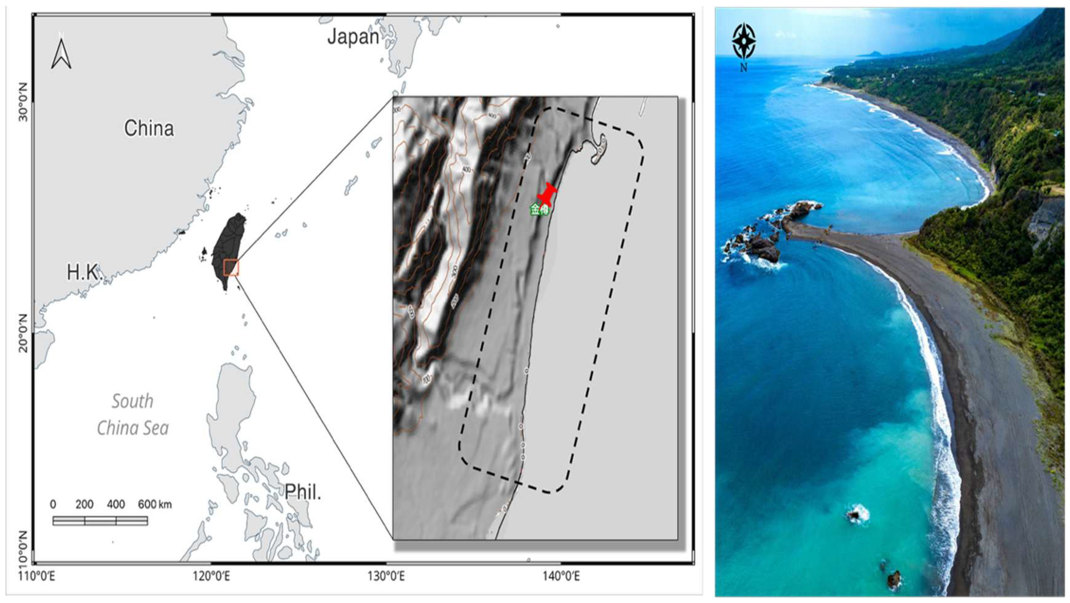
Taitung, situated in the southeastern part of Taiwan, is renowned for its rugged coastal topography, which is constantly being shaped by frequent seismic activity, typhoons, and wave dynamics, resulting in the formation of towering sea cliffs and narrow coastal plains. The specific area used to test the warning system framework proposed in this study is Jinzun Beach (Figure 1, dashed line). The beach spans approximately one kilometer in length, with a shoreline inclination of approximately 10 degrees clockwise from north. The surf zone in this area is about 200 m wide, and the incident waves are shore normal. Jinzun is well known for its picturesque scenery, characterized by azure waters, captivating waves, and the presence of a nearby land-tied island, making it a popular destination for photography enthusiasts. However, public access to this pristine beach is restricted. Visitors can only observe the beach from a docking station located at the Jinzun Recreation Area, marked by the red pin in Figure 1. This recreational area provides an elevated point that offers panoramic views of the entire beach. The Taitung government has installed a pan–tilt–zoom webcam at this site, allowing individuals to remotely enjoy the scenic views. Across Taiwan, numerous beaches exhibit similar conditions to Jinzun Beach, where public access is restricted or routine patrol services are absent. Webcams have been deployed to facilitate continuous enhanced coastal monitoring.

The webcam installed at Jinzun Recreation Area features an optical zoom function and can record videos at a maximum frame rate of 60 frames per second (FPS) with a resolution of 1290 × 1080 pixels. This combination of a high frame rate and resolution enables the camera to capture videos that are both fluid and sharp. The camera periodically rotates to capture the entire beach and zooms in on the beach as well as the adjacent sea. However, although the camera remains fixed at the recreation area, its viewing angle changes every less than two minutes, which constrains its effectiveness for continuous monitoring. To enhance our observations, we set up a timelapse camera near the webcam. This timelapse camera was set to capture one frame per second, enabling continuous footage to be recorded from a fixed orientation towards the south. The features and settings of the cameras can be found in

Table 2. Camera specifications.

Webcam (Model: DJS 6SIP225E)	Timelapse (Model: Brinno TLC200Pro)
Government-owned	Deployed for this study
Tilt–pan–zoom functionality	Stationary, facing south
Resolution: 1920 × 1080	Resolution: 1280 × 720
30~60 FPS	1 FPS (manual setting)
Public access to the videos	Limited access (study-specific)

.

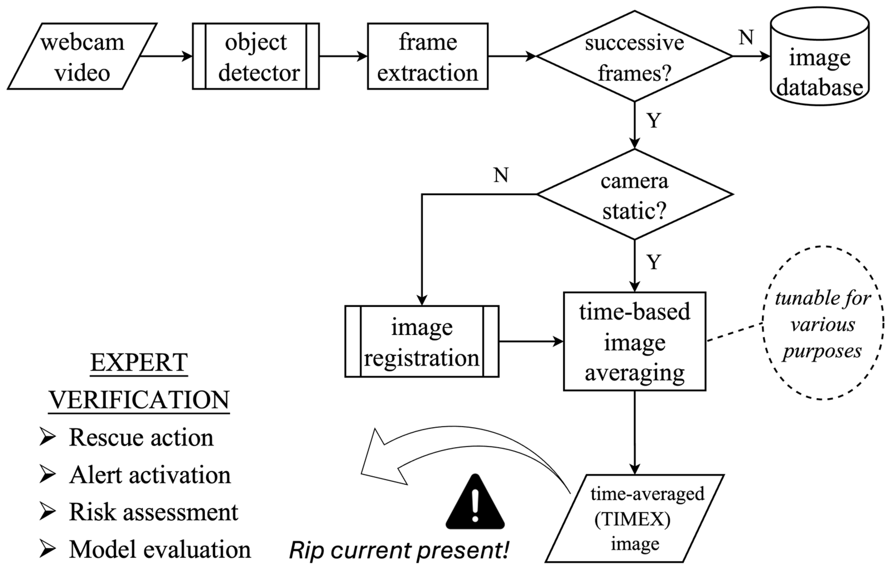
The overall process of the proposed rip current warning system framework is shown in Figure 2. The intended primary data source for this system is the video footage captured by coastal webcams. These videos are analyzed by an object detector trained to identify channel rips. Following positive detections by the object detector, the corresponding frames are extracted and evaluated against the predefined consecutive-frame criteria to ensure they represent a coherent rip current event. Any non-consecutive detections are stored for future model refinement. For the valid event frames, image registration was conducted by applying Speeded-Up Robust Features (SURF) technique [38] to detect and match invariant keypoints, followed by geometric transformation estimation and image resampling. The registered frames are then averaged pixel by pixel over time, producing the final time-averaged (TIMEX) [39] image for expert verification and operational decision-making.

2.2. Training Data

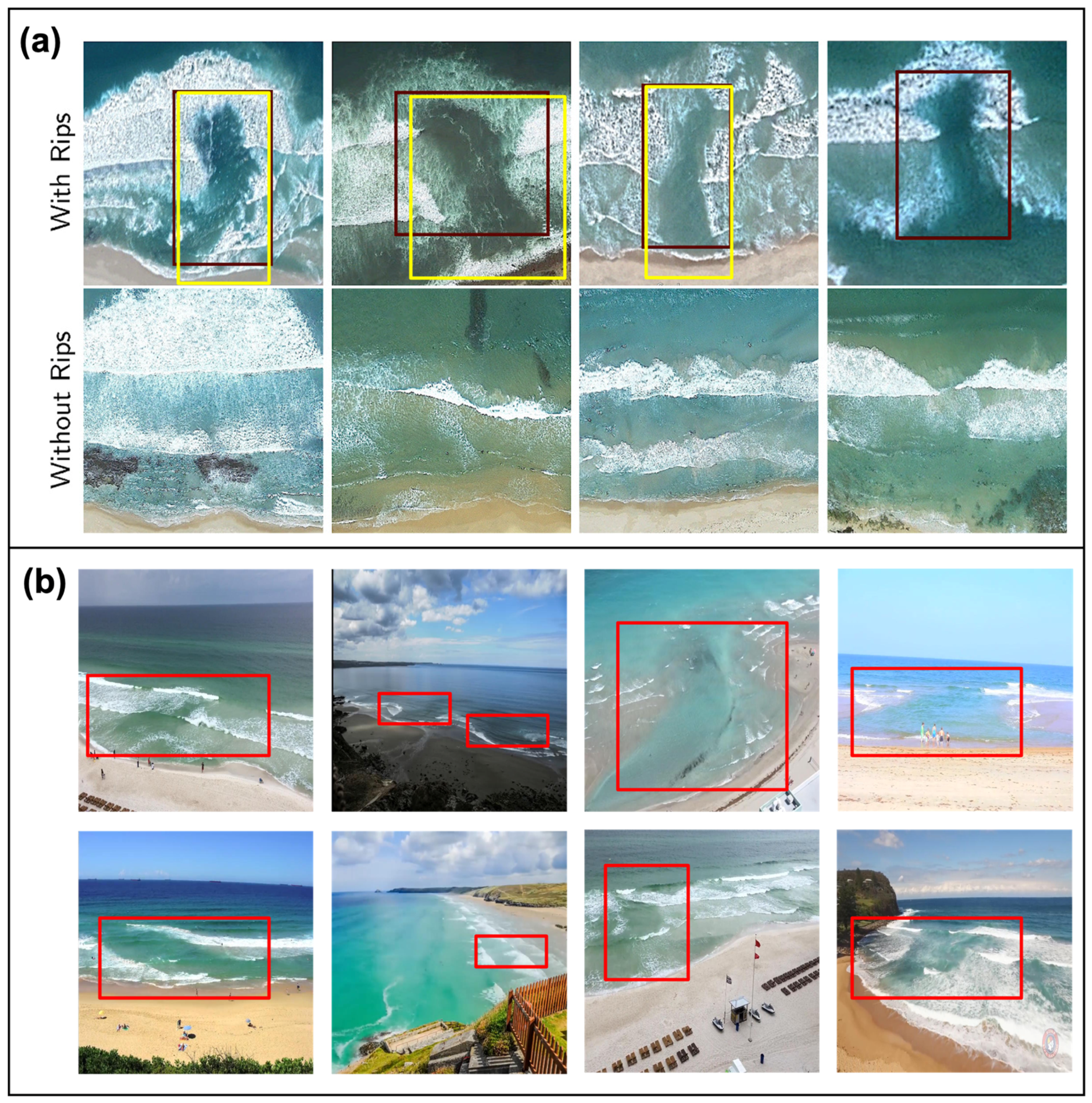
The acquisition of a sufficient number of high-quality images represents a critical prerequisite for the development of robust object recognition modules. To address this requirement, two primary sources were employed to build a comprehensive rip current image database. The first source comprises a publicly available dataset provided by de Silva et al. [23], containing 1740 images with rip currents and 700 images without rip currents. The channelized rip current annotations within this dataset were validated by a rip current expert from the National Oceanic and Atmospheric Administration (NOAA). Consequently, this dataset is hereinafter referred to as the NOAA data. As shown in Figure 3a, the NOAA data consist of aerial imagery sourced from Google Earth.

A key component of the present research was comprehensive data cleaning and relabeling procedures to improve the dataset’s quality and applicability. Data cleaning, which involves identifying and removing noisy or irrelevant images, constitutes a crucial step in machine learning workflows, as unrefined data can significantly compromise model performance [40,41]. Beyond the cleaning process, the original annotations of the NOAA data (Figure 3a, red boxes) were refined by expanding the bounding boxes to include portions of adjacent beach areas (Figure 3a, yellow boxes). This modification was implemented to better represent real-world conditions, particularly for future applications involving coastal surveillance camera systems, where rip currents are often observed within the broader context of beach environments.

While valuable, the NOAA dataset contains only aerial imagery, which limits its representativeness of real-world, ground-level perspectives. To overcome this limitation and enhance both the diversity and quantity of training samples, an additional dataset—referred to as the BEACH data—was compiled. This dataset includes 1197 images with rip currents and 100 images without rip currents, collected from coastal video footage, rip current educational materials, and web-based imagery. The BEACH data feature both aerial and beach-level views, and the image resolutions vary from 1280 × 720 to 450 × 338 pixels. Rip currents were labeled using axis-aligned bounding boxes. Prior to training, the dataset underwent a data cleansing procedure to remove duplicate or visually ambiguous samples. The annotations were reviewed by multiple members of the research team to ensure labeling consistency. Representative examples are shown in Figure 3b. The composition and key characteristics of the three datasets are summarized in

Table 3. Summary of the training datasets.

Dataset	Total Images	With Rip	Without Rip	Image Size (Pixels)	Annotation Description	Data Source
NOAA	2440	1740	700	234 × 234 to 1110 × 1000 (most images cropped to square format)	Original bounding boxes	de Silva et al. (2021) [23]
Refined-NOAA	2440	1740	700		Expanded Bounding Boxes
BEACH	1297	1197	100	450 × 338 to 1280 × 720	Axis-aligned bounding boxes	Collected in this study from publicly accessible web imagery, video footage, etc.

. A summary of the BEACH dataset metadata is available in the Appendix A.

All datasets were partitioned at the image level into training, validation, and test subsets using a consistent 8:1:1 ratio. Subsequently, seven data augmentation strategies were applied to the training subsets. These augmentation methods were designed to simulate the physical and optical variability commonly observed in coastal environments, incorporating both geometric and photometric transformations:

• Horizontal flipping: This transformation aims to represent rip currents as they might appear under different shoreline orientations.
• Scaling: This adjustment accounts for variations in the distance between the camera and the surf zone.
• Translation: This technique simulates minor camera shifts or vibrations caused by wind.
• Rotation: This transformation addresses potential camera tilt or non-parallel horizons.
• Shearing: This method mimics perspective distortions caused by oblique viewing angles or variations in camera mounting height.
• Hue, saturation, value (HSV) transformation: This adjustment alters hue, saturation, and brightness to simulate a range of illumination conditions, including intense midday glare, low-contrast overcast scenes, and reduced visibility at dawn or dusk.
• Mixed: In addition to the six transformations mentioned above, an eighth method was implemented. This approach randomly selects and applies two of the seven primary transformations, generating more complex synthetic scenarios.

2.3. Object Detector Development

To develop an object detector capable of identifying rip currents from video data, we primarily focused on selecting a deep learning model that delivers high recognition speeds while maintaining a satisfactory accuracy. In real-time applications, the chosen model must sustain a frame rate exceeding the standard video rate of 30 FPS [42]. To guide model selection, benchmark evaluations on the MS COCO dataset using the Nvidia GPU V100 (Nvidia, Santa Clara, CA, USA)were performed to provide comparative insights into the performance characteristics of various detector architectures [43]. Object detection models can generally be categorized as two-stage or one-stage architectures. Two-stage detectors, such as Feature Pyramid Networks (FPNs) and Neural Architecture Search (NAS) networks, first generate object proposals before performing classification and localization [44,45]. While these models often achieve superior detection accuracy, their sequential processing leads to slower inference speeds, making them less suitable for real-time scenarios [46,47]. In contrast, one-stage detectors like EfficientDet and YOLO execute detection over a dense grid of potential object locations in a single pass, offering substantial improvements in processing efficiency [48,49].

Among one-stage detectors, the YOLO network family demonstrates a particularly balanced compromise between speed and accuracy for real-time applications. Originally proposed by Joseph Redmon and Santosh Divvala in 2016 [48], YOLO has undergone continuous optimization through multiple iterations [50,51]. At the time of system development and pilot field deployment in late 2022, YOLOv4 was a stable and widely documented implementation within the series [52]. It has been successfully adapted across diverse real-time detection scenarios, including the identification of uneaten feed pellets in underwater images, the recognition of traffic signs, the detection of targets in UAV imagery, and the identification of fires in surveillance systems [53,54,55,56]. The primary objective of this study is to design and validate a rip current warning framework that integrates real-time object detection with a temporal averaging mechanism to address the complexities of dynamic sea conditions. During system development, YOLOv4 was selected as a reliable and well-supported backbone, providing the necessary real-time performance for operational deployment.

To evaluate the effectiveness of the model, four metrics derived from the confusion matrix were utilized: precision, recall, F1-score, and average precision (AP). Precision evaluates the accuracy of the model’s positive predictions, as represented by Equation (1)

$$\mathrm{P}\mathrm{r}\mathrm{e}\mathrm{c}\mathrm{i}\mathrm{s}\mathrm{i}\mathrm{o}\mathrm{n}={\displaystyle \frac{\mathrm{T}\mathrm{P}}{\left(\mathrm{T}\mathrm{P}+\mathrm{F}\mathrm{P}\right)}}$$

(1)

where true positive (TP) represents the number of instances correctly identified as positive by the model, and false positive (FP) represents the number of instances incorrectly identified as positive when they are negative. A high precision value indicates that the model produces fewer false alarms. Recall indicates the ability of a model to identify all the relevant cases of actual positive instances, as shown in Equation (2). False negative (FN) in Equation (2) denotes the number of instances incorrectly identified as negative when they are positive.

$$\mathrm{R}\mathrm{e}\mathrm{c}\mathrm{a}\mathrm{l}\mathrm{l}={\displaystyle \frac{\mathrm{T}\mathrm{P}}{\left(\mathrm{T}\mathrm{P}+\mathrm{F}\mathrm{N}\right)}}$$

(2)

While precision and recall are metrics widely used to evaluate a model, a tradeoff between these two metrics is unavoidable in retrieval performance [57]. Therefore, the F1-score was established to simultaneously measure precision and recall and evaluate the overall model performance [58]. Mathematically, the F1-score is the harmonic mean of the precision and recall, as shown in Equation (3).

$$\mathrm{F}1-\mathrm{s}\mathrm{c}\mathrm{o}\mathrm{r}\mathrm{e}={\displaystyle \frac{2\times \mathrm{P}\mathrm{r}\mathrm{e}\mathrm{c}\mathrm{i}\mathrm{s}\mathrm{i}\mathrm{o}\mathrm{n}\times \mathrm{R}\mathrm{e}\mathrm{c}\mathrm{a}\mathrm{l}\mathrm{l}}{\left(\mathrm{P}\mathrm{r}\mathrm{e}\mathrm{c}\mathrm{i}\mathrm{s}\mathrm{i}\mathrm{o}\mathrm{n}+\mathrm{R}\mathrm{e}\mathrm{c}\mathrm{a}\mathrm{l}\mathrm{l}\right)}}={\displaystyle \frac{2\mathrm{T}\mathrm{P}}{2\mathrm{T}\mathrm{P}+\mathrm{F}\mathrm{P}+\mathrm{F}\mathrm{N}}}$$

(3)

The F1-score is a crucial measure for assessing the trade-off between precision and recall. Nevertheless, it tends to give more weight to lower precision or recall [59]. Consequently, the average precision (AP) metric is also widely employed to assess the model’s performance, shown in Equation (4) [60].

$$AP={\int }_0^{1}P\left(R\right)dR$$

(4)

where P(R) is the precision at a specific recall level r. The integral is taken over all recall values from 0 to 1. AP quantifies the precision–recall performance of a model by integrating the Precision–Recall Curve (PRC) and provides a comprehensive measure of a model’s ability to make high-confidence predictions while maintaining a high recall across various confidence thresholds.

2.4. Image Averaging and Registration

Time-averaged imagery (TIMEX [39]) has proven valuable for studying wave breaking patterns in coastal areas [27,61,62,63]. This technique works by averaging successive video frames of the same scene over a specific duration, which attenuates dynamic elements such as individual waves while preserving their mean brightness patterns. Persistent oceanographic features, such as rip current channels, become visible in averaged images as dark regions extending across the surf zone. In this study, the time-averaging approach is adopted to address a fundamental challenge in automated rip current detection. Object detection models are designed to identify features within individual video frames, but rip currents present a unique difficulty because their characteristics are often not readily apparent in single frames. The transient and dynamic nature of these currents means that frame-by-frame analysis can produce highly variable results, with the model potentially identifying different locations or missing the feature entirely from one moment to the next.

To overcome this limitation, in this study, time averaging was applied not to the raw video footage but to the model’s inference results themselves. Rather than triggering an alarm based on detection in any single frame, multiple frames where the model has identified potential rip currents are processed. The methodology works as follows: when the model generates positive detections with bounding boxes across a video sequence, those specific frames are extracted and averaged over the analysis period. If a genuine rip current is present, its characteristic dark channel is expected to appear persistently across the sequence of frames and thus to be distinctly visible in the resulting time-averaged image. Correspondingly, bounding boxes predicted by the detection model may remain evident in the averaged output, indicating consistent and reliable identification. In contrast, the disappearance of bounding boxes in the composite image suggests temporal inconsistency and potentially spurious detections. This temporal aggregation process therefore functions as a validation mechanism, enabling the assessment of the model’s inference reliability prior to further analytical or operational application.

Typically, the time-averaging technique involves recording a series of images depicting a consistent scene to ensure the relevance of the averaged information and to mitigate random noise or variability. However, this study employs real-world data acquired from pan–tilt–zoom monitoring webcams. The movement of the camera causes a misalignment in the sequence of images, and thus, averaging these images may yield a composite image that is blurred or unclear. Consequently, it is necessary to register images prior to averaging. The image registration procedure follows the four stages outlined by Zitova and Flussersser [64]: feature detection, feature matching, model estimation, and image transformation. Speeded Up Robust Features (SURF) [38] technique is used to detect and match key points between two frames. Based on these matched correspondences, a projective transformation homography is estimated to model the geometric relationship between the images. The resulting homography matrix is subsequently applied to warp the image coordinates, followed by interpolation-based resampling to generate the aligned frame.

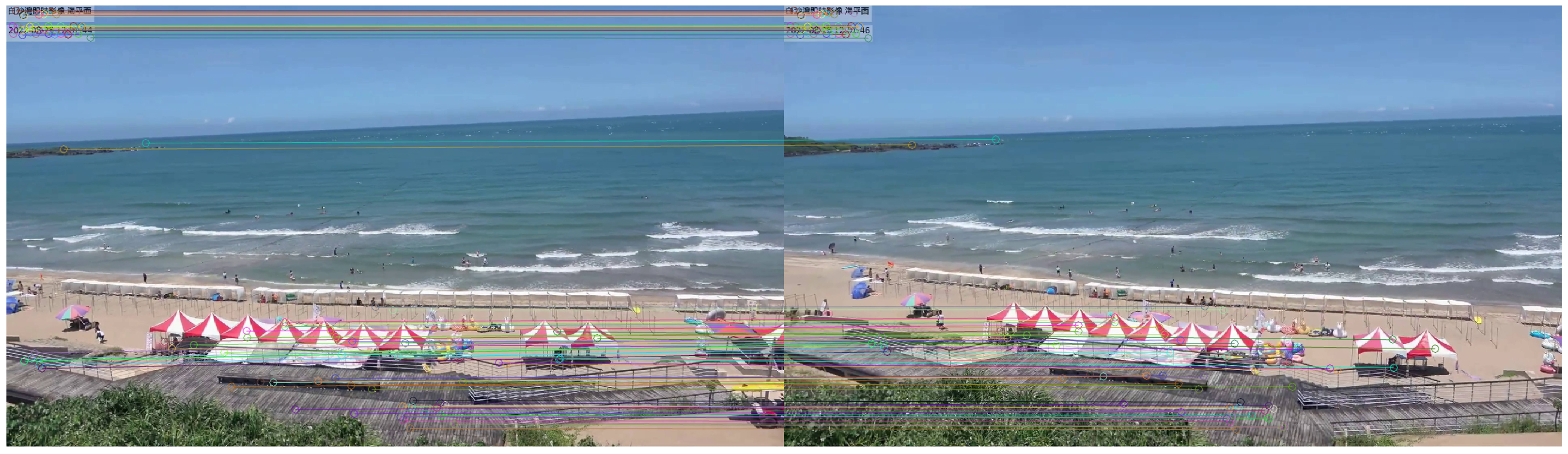
Among these stages, feature detection and matching constitute the most computationally intensive components. Thus, the entire registration workflow was developed in this study using a custom program designed to adjust the number of matched feature points for various beach environments and scene complexities. Figure 4 presents an example output from the registration program, showing the matched key points between two frames captured during camera rotation. The left image serves as the reference, while the right image is aligned with it. Circular markers indicate detected feature points, while connecting lines show matched pairs identified by the SURF algorithm.

2.5. Criteria of the Consecutive Frames

When the detector identifies rip current features, it extracts the segmented frames from the video. Since the model processes 40 frames per second, numerous segmented frames can be captured during a single rip current event. In this study, consecutive frames are defined as all segmented frames detected during a single rip event to differentiate between frames from separate occurrences. Two criteria are used to define consecutive frames: a minimum time separation of 8 s and a maximum averaging duration of 30 s. A TIMEX image is generated when either of these criteria is met. Although these temporal parameters were optimized for the current dataset and study site, the proposed framework is designed to be flexible. In practical applications, the minimum separation threshold and the maximum averaging window can be adjusted based on sea-state characteristics, such as the dominant wave period, or specific deployment purposes, to ensure the resulting TIMEX visualization remains representative.

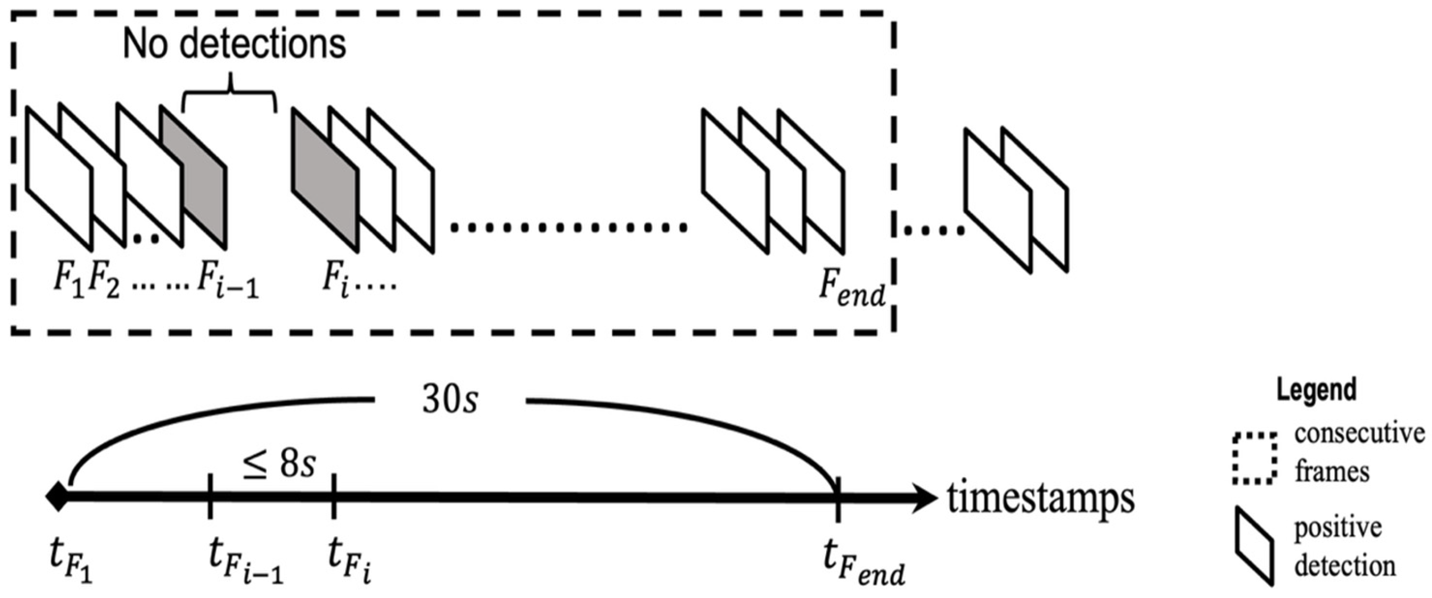
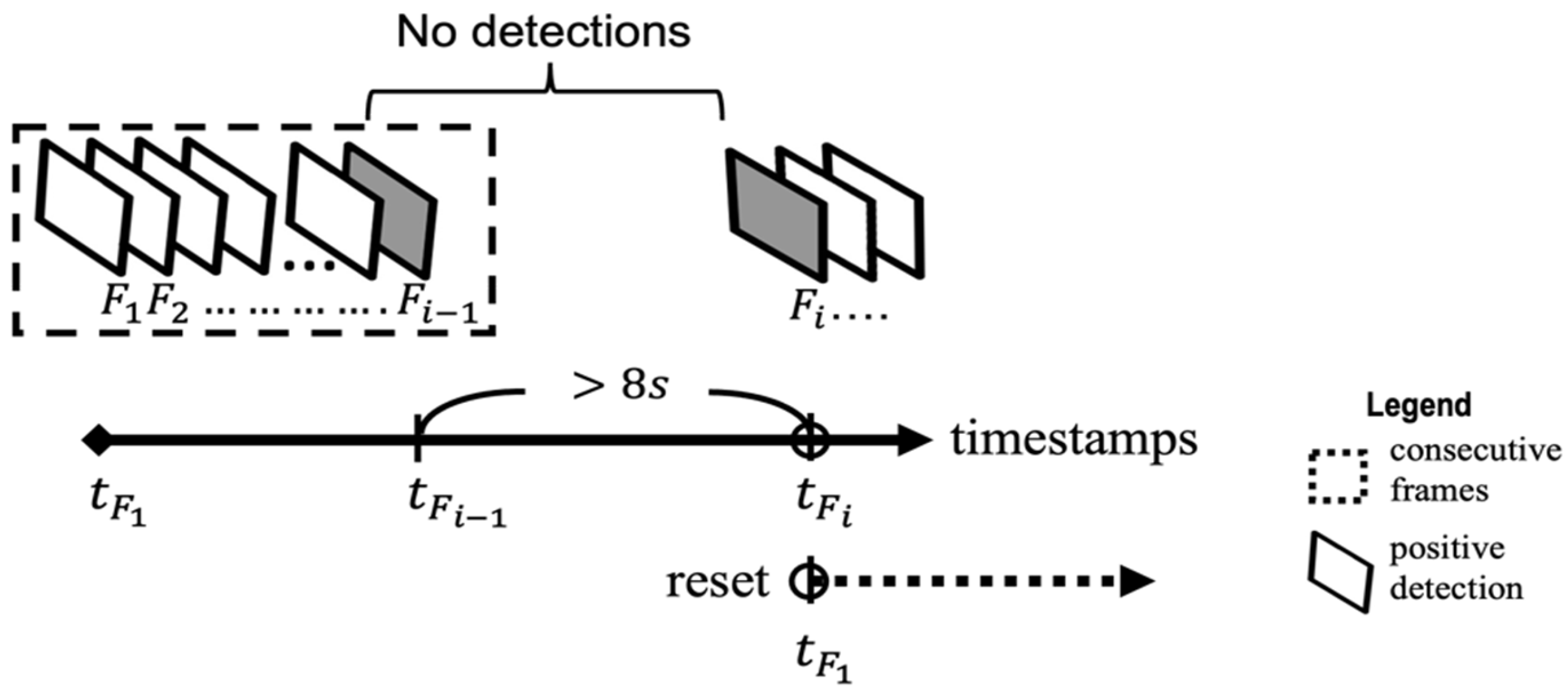
The occurrence of rip currents is directly influenced by wave properties. In the study area, the predominant wave period is 8 s. This wave period is used as a temporal threshold to differentiate between rip current events. Specifically, when two detected rip current are separated by more than 8 s, they are classified as distinct events rather than continuations of the same occurrence. Figure 5 illustrates the minimum criteria for identifying rip current events from webcam video frames. Let $F_1,F_2,\dots ,F_i$ denote the sequence of frames in which rip currents are detected, and let their corresponding timestamps be represented as $t_{F_1},t_{F_2},\dots ,t_{F_i}$. The system designates $t_{F_1}$ as the initial timestamp, marking the onset of a rip current event. Upon each new positive detection, the system computes the temporal interval between the current and next detection. If the calculated interval is less than or equal to 8 s, the current detection $F_i$ is considered to belong to the same rip current event. Conversely, if the temporal interval exceeds 8 s, the system interprets this as the initiation of a distinct event. The event window is re-initialized in such cases by setting $t_{F_1}$ equal to $t_{F_i}$. All frames that occurred before this reset are categorized as consecutive frames. This indicates a coherent sequence of detections of the same event over time.

While the 8 s minimum threshold ensures that each frame in the set of consecutive frames contributes meaningful information to the same rip current event, another maximum averaging time (the 30 s) criterion is used in our research to select consecutive frames. This criterion functions similarly to traditional averaging methods by capping the length of data being averaged. We set the maximum average time to 30 s because typical wind and swell wave periods are shorter than 30 s. Additionally, 30 s is a crucial amount of time for rescue operations, as will be discussed further in the Section 4. Figure 6 illustrates how the 30 s maximum averaging window is applied in rip current event detection. The process for selecting consecutive frames begins similarly to the method used to evaluate the minimum separation interval: the system calculates the time interval between each new detection and the previous one. In addition to this, it also determines the total time elapsed between the current frame and the starting frame of sequence $F_1$. At this stage, $F_1$ serves as the reference point for determining the maximum allowable duration of a single event. When the time difference between $F_i$ and $F_1$ exceeds 30 s, the system designates the current frame as $F_{end}$, and all preceding frames from $F_1$ through $F_{end}$ are grouped together as a single set of consecutive frames. After this, the reference point $F_1$ is reset to the next detected frame, and the process begins again.

3. Results

Three distinct models were developed, each trained on datasets with varying compositions to assess the influence of data diversity on detection performance. The models were trained with an input resolution of 416 × 416 pixels, a batch size of 64, max_batches set to 8000, and an initial learning rate of 0.001. A detection was considered valid when the Intersection over Union (IoU) exceeded 0.5. Training and inference were performed on a workstation configured with an Intel Core i7-10700 @ 2.9 GHz CPU, 32 GB RAM, and an NVIDIA RTX 3090 GPU (24 GB), supported by CUDA 10.0 and cuDNN 7.0. Under this environment, the optimized BEACH model achieved an inference speed of approximately 40 FPS, exceeding the standard 30 FPS requirement for real-time video processing.

3.1. Model Evaluation

The model performances were assessed across multiple quantitative metrics, as summarized in

Table 4. Model performance matrix.

Training Data	Recall	Precision	F1-Score	AP
NOAA	64%	81%	71%	75%
Refined-NOAA	62%	80%	70%	72%
BEACH	81%	91%	87%	92%

. The NOAA and Refined-NOAA models demonstrated comparable performance, exhibiting only minor differences in accuracy metrics—less than 3 percent—arising from the limited modifications made to the original NOAA dataset labels. In contrast, the BEACH model demonstrated superior performance, achieving a precision of 91%, a recall of 81%, an F1-score of 87%, and an average precision of 92%. This model consistently surpassed the other two across all evaluated metrics, positioning it as the most robust and effective choice among the trio. The enhanced performance of the BEACH model is likely attributed to its larger dataset, which offers a more extensive range of imagery for training.

As summarized in

Table 5. Detection outcome summary derived from confusion matrices. TP, FP, and FN rates are computed by normalizing to the number of ground-truth bounding boxes.

Datasets	TP	FP	FN
NOAA	64%	19%	36%
Refined-NOAA	62%	20%	38%
BEACH	81%	9%	19%

, the BEACH model exhibited a False Negative (FN) rate of 19%, representing a clear reduction compared with the 36%, 38% FN rates observed in the NOAA-based models. Because channelized rip currents are typically characterized by spatial persistence and temporal stability, occasional missed detections in isolated frames are unlikely to compromise the identification of sustained rip current features. Within the precision–recall trade-off, the model was trained to prioritize precision, aligning with the operational needs of lifeguards and beach managers who require reliable information.

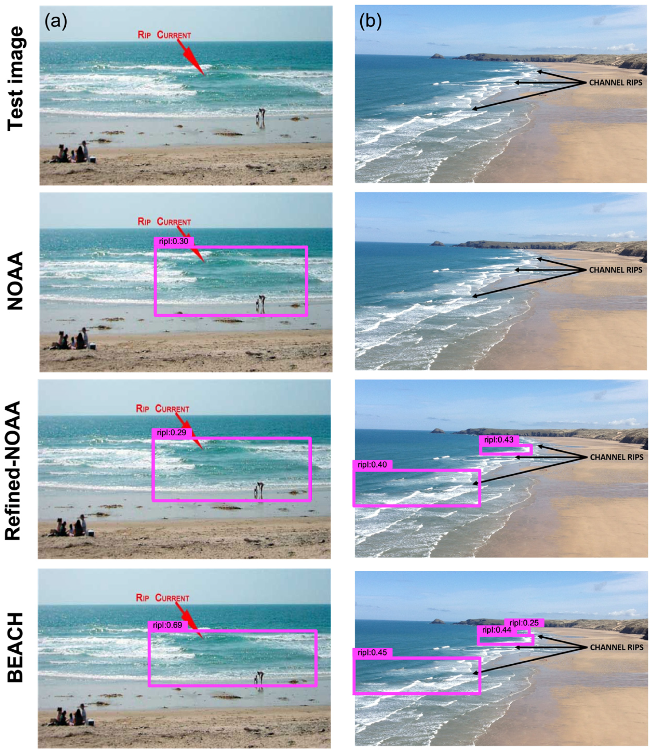
Relying solely on numerical metrics may not comprehensively capture a model’s efficacy in real-world scenarios; thus, we analyzed differences in prediction using two test images. Figure 7a [65] shows a straightforward case with a distinctly visible dark rip current channel against white breaking waves and brown sand. In contrast, Figure 7b [29] presents a more complex scenario where the rip current occupies a smaller portion of the image. Both images, extracted from an educational site and journal article, respectively, include marked rip current locations that serve as ground truth references for evaluating our model predictions. The prediction results in Figure 7 demonstrate that all three models—NOAA, Refined-NOAA, and BEACH—successfully identified the rip currents in the simpler Figure 7a scenario. However, for the more challenging Figure 7b, the Refined-NOAA and BEACH models outperformed the standard NOAA model. Notably, the BEACH model also demonstrated a superior detection capability compared to the Refined-NOAA model, successfully identifying three rip currents present in Figure 7b, while the Refined-NOAA model detected only two. This suggests that the refined labeling approach used during training enhanced the model’s ability to recognize rip currents in complex environments in which the rip current occupies a smaller proportion of the image compared to the surrounding breaking waves and background elements.

3.2. Rip Current Detection in Videos

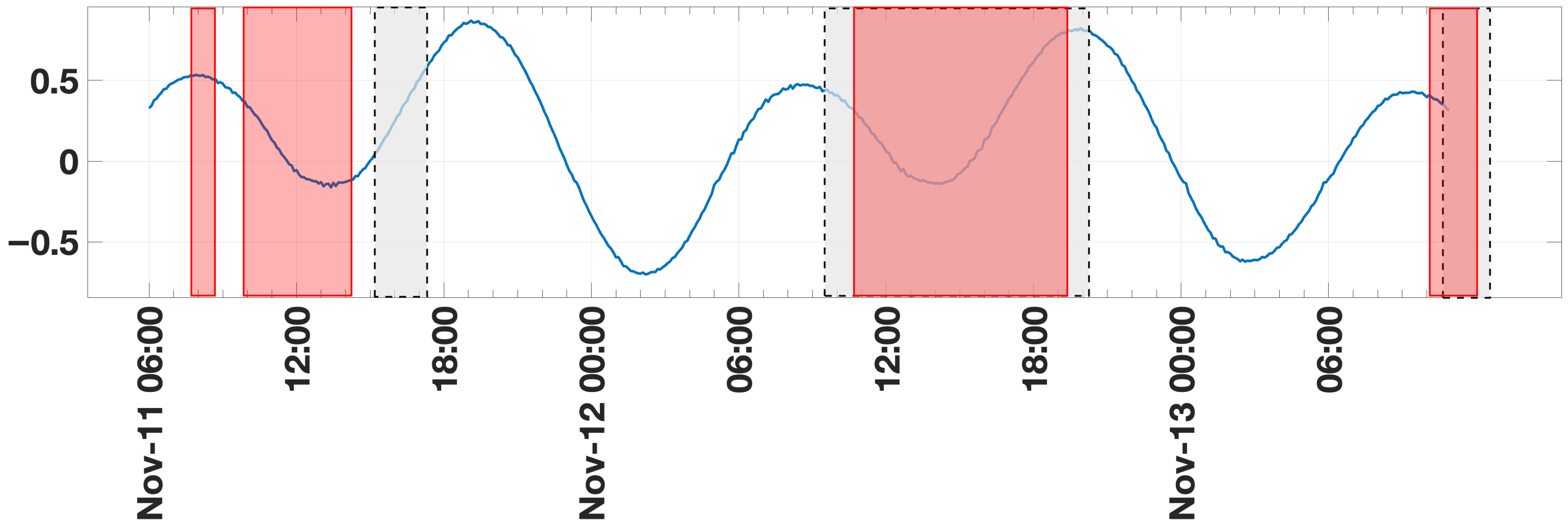
Timelapse videos were recorded during daylight hours from 11 November to 13 November 2022, at the Taitung Jinzun Recreation Area in Taiwan. The timeframe of these recordings is depicted in Figure 8 within the indicated red boxes. Additionally, we obtained videos from government-operated webcams, with the corresponding recording times detailed in the gray boxes in Figure 8. These video data represent the real-world scenarios used to assess the performance of our model and the reliability of our warning system framework. The blue curve in Figure 8 represents the normalized tidal height.

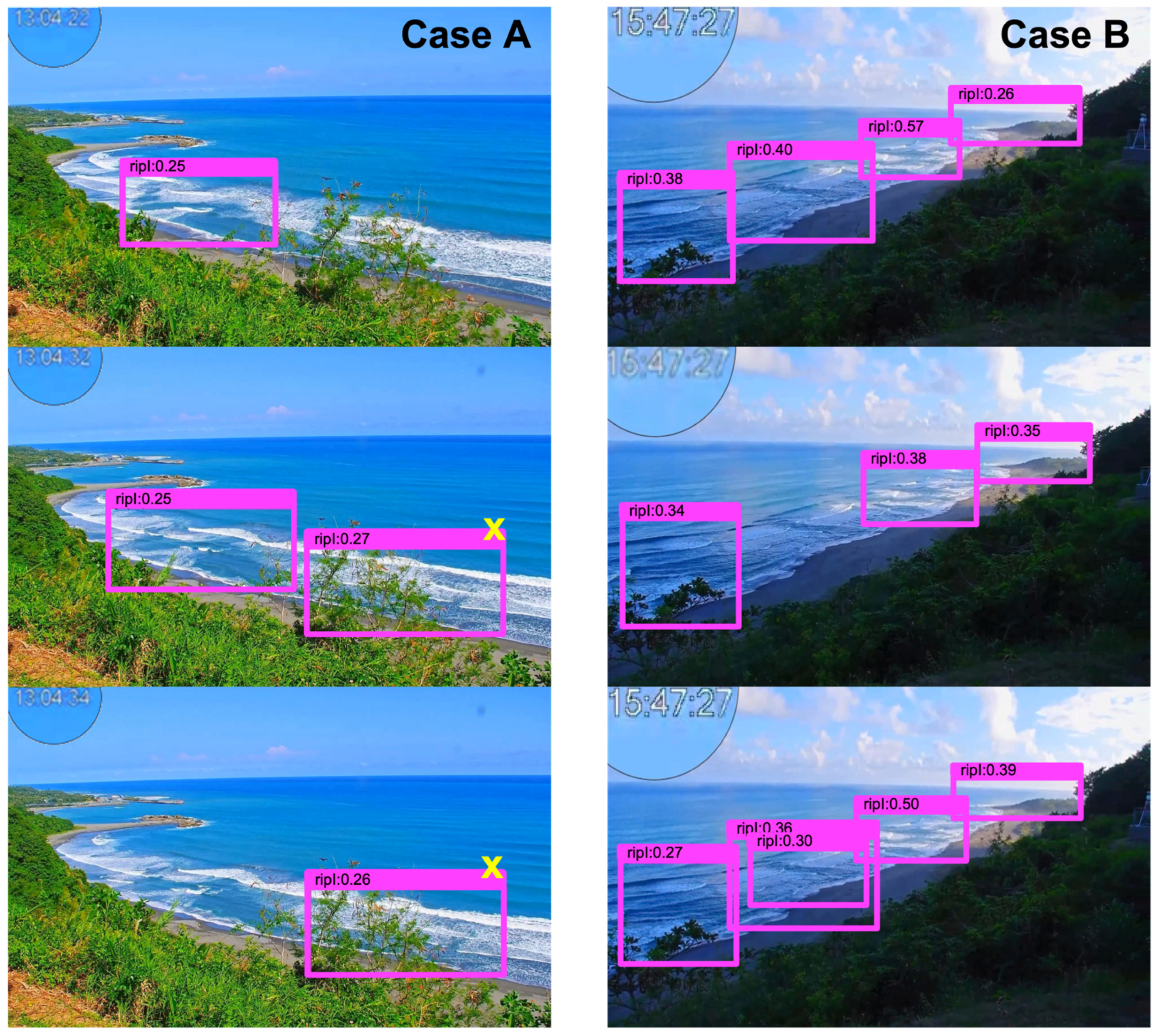
The BEACH model, identified as the most effective model in previous investigations, was employed to detect rip currents in the video data. Figure 9 displays two examples of the model’s predicted results. Each image in Figure 9 is a frame extracted from the results of the inference process. The bounding boxes highlight the regions where the model has identified dark channel patterns associated with rip currents. Given that the camera is positioned slightly north of the beach’s center and rotates horizontally along the north–south axis, the perspectives captured in the images of the northern (Case A, on the left side of Figure 9) and the southern (Case B, on the right side of Figure 9) areas of the beach differ. Since the BEACH model processed the video at a speed that exceeded the frame rate of 30 FPS, it generated numerous positive detections of rip currents within each one-minute recording interval for both cases. Due to the large volume of detections, only three representative frames from each case are shown in Figure 9. The timestamps of these frames are sequential but not continuous. The top images in Figure 9 are the earliest, followed by the middle and the bottom images, which represent the latest timestamp. During video recording, we also conducted simultaneous visual observations of the beach, and in both cases, rip currents were indeed present and visible to the naked eye.

Case A captures the northern section of the beach at 1:04 PM on November 11, under clear skies, with only a few clouds creating shadow patterns. In Case A, the model correctly identifies a rip current channel near the center-left area of the beach in the earliest frame. This channel exhibits typical visual characteristics of a rip current, such as a gap in the breaking waves and darker water. In the middle frame, the same rip current region remains detected, showing consistent recognition, but the model incorrectly identifies a false positive near the far right of the beach, marked by an “x”. This false positive also appears in the last frame of Case A. These false positives likely result from image artifacts or obstruction. For example, the view is partially blocked by vegetation, along with transient or breaking wave shadows that resemble the dark features of rip currents, leading the model to mistakenly classify the area as a rip current. Case B depicts the southern section at 3:47 PM on the same day, with overcast skies and reduced lighting. In Case B, despite the webcam’s timestamp resolution being limited to one-second intervals (15:47:27), the model generates frame-specific predictions within each second and maintains accurate detection throughout the sequence, though this results in detection variability among frames with identical timestamps. Four distinct channels of rip currents were detected throughout the sequence. While the locations of the detected rip currents remain consistent and accurate, there are minor variations in the dimensions of the bounding boxes across consecutive frames. These variations occur as the model responds to temporary changes in the surf zone characteristics, such as changes in foam distribution and lighting conditions. The model’s sensitivity to these visual similarities highlights its capability to capture changes in the dynamic surf zone environment while detecting the fundamental structures of rip currents.

However, for rip current warning systems, relying on real-time detection results to trigger alerts can result in an excessive number of warnings or false alarms, leading to alarm fatigue among users. A reliable alarm system should accurately represent the true patterns of rip current activity, giving users a clearer understanding of when danger is imminent. Therefore, we use a time-based averaging technique to generate a TIMEX image that acts as a reference for alarm activation.

3.3. Time-Based Image Averaging

While time-averaging techniques have been employed in various studies on rip currents, most of these studies typically extracted images at regular, predetermined time intervals and computed the average pixel values across these frames to produce a single averaged output. In contrast, in our research, we take a unique approach by selectively averaging only the frames in which the model has indicated a positive detection. Additionally, we established two criteria for maximum and minimum durations for the averaging time, which can be adjusted based on the characteristics of rip currents at different beaches. As a result, non-fixed time intervals are used in our averaging process, enabling a more dynamic and context-specific assessment.

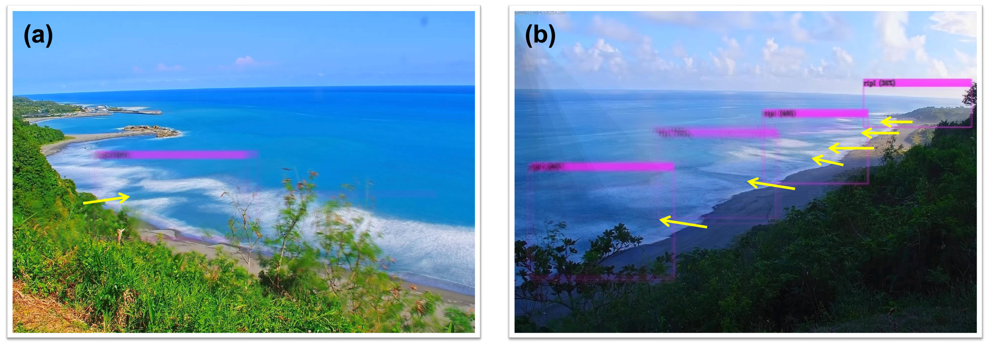
This specialized averaging method offers two key advantages. Firstly, it effectively filters out potential false positives generated by the model. Taking Case A in Figure 9 as an example, even though the model predicted some false positives, when applying our temporal averaging technique, these false detections become nearly imperceptible in the resultant TIMEX image (Figure 10a). Meanwhile, the model’s prediction emerges as a prominent bounding box that correctly identifies the genuine rip current channel, as confirmed by the researcher-drawn arrow in Figure 10a. Suppressing these false detections before they can trigger warnings ensures that users receive alerts only when rip currents are consistently present, thus maintaining user trust in the system. Secondly, our averaging method provides an effective means to evaluate the model’s real-world performance.

In Figure 9, the second bounding box on the left side of Case B exhibits noticeable variations in position and size across frames. These fluctuations pose challenges for a rip current alarm system; however, the averaging process mitigates this issue. In the resulting TIMEX image (Figure 10b), the second bounding box on the left side appears hazier and more diffused than the other three because it is a combination of multiple frames with shifting detections. Despite this reduced clarity, the rip current channel is still correctly identified within the averaged box, ensuring that genuine threats are not missed while preventing the system from issuing erratic or contradictory warnings. Importantly, the varying visual clarity in the TIMEX image reflects the model’s variable confidence and provides experts with crucial information for making alarm decisions. By distinguishing between sharp, well-defined detections and hazier, less stable ones, experts examining the TIMEX images can better assess which detections warrant immediate alerts and which require further observation, ensuring that warnings are issued based on robust, well-supported evidence rather than transient or uncertain predictions. Additionally, these visual characteristics provide valuable diagnostic information for identifying areas where the model performance requires refinement, enabling continuous improvement of the alarm system’s accuracy over time.

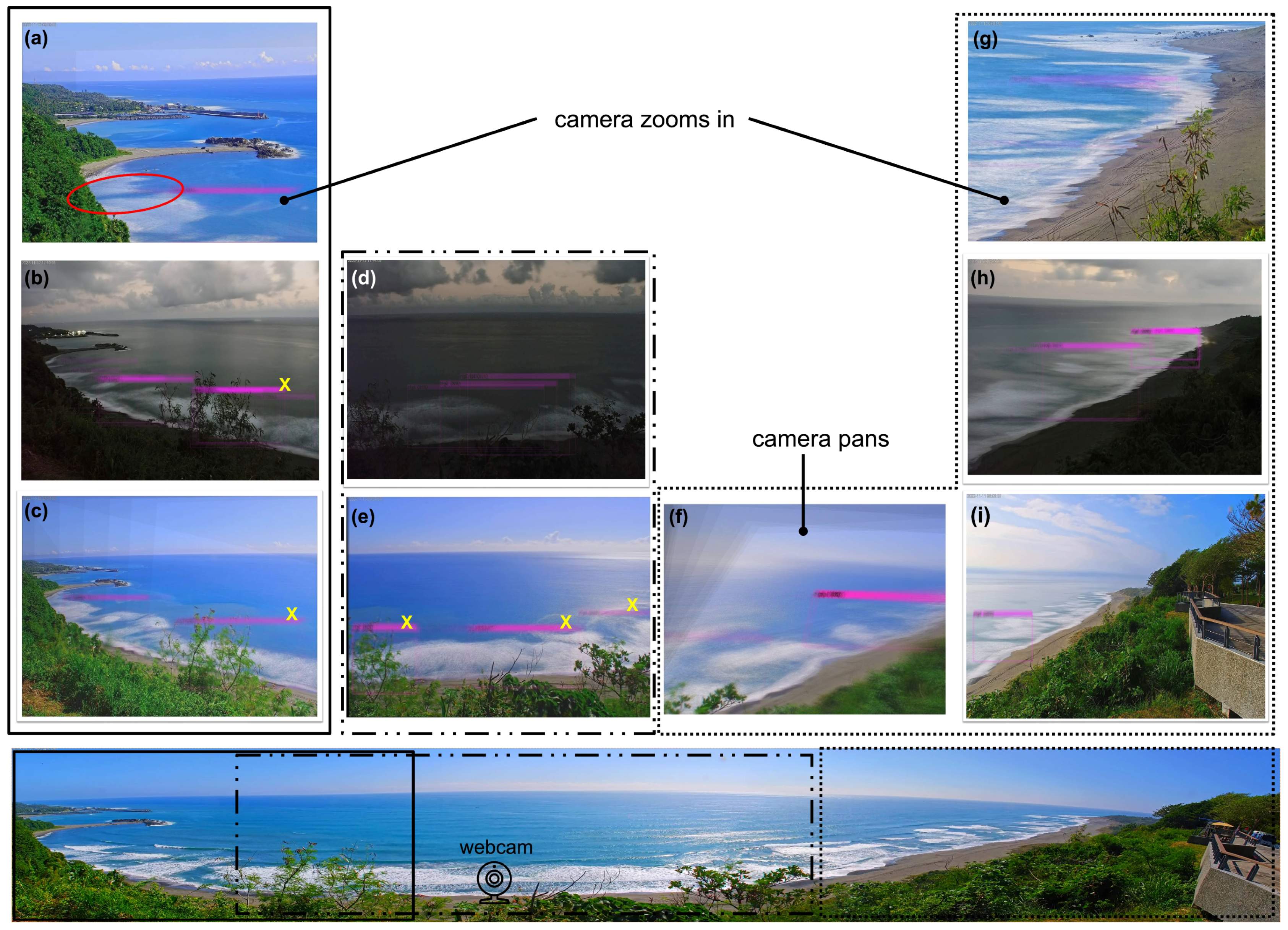
For an overall examination of the performance in the detection of rip current channels across different beach sections, Figure 11 presents representative TIMEX images alongside a panoramic image. The rectangular regions correspond to the northern (solid line), central (dash–dot line), and southern (dotted line) beach sections captured within fixed observational fields of view. The accompanying TIMEX imagery is organized by location: northern section (Figure 11a–c), central section (Figure 11d,e), and southern section (Figure 11f–i). Two special TIMEX types are highlighted: “zoomed-in” TIMEX images (Figure 11a,g), generated when the camera automatically zoomed in and paused at the northernmost and southernmost positions, and a “panning” TIMEX image (Figure 11f), generated during active camera rotation between viewing angles.

The deep learning model demonstrates superior performance in the southern section compared to the northern section, which can primarily be attributed to vegetation interference and the spatial characteristics of each camera view. Coastal vegetation along the northern coastline blocks part of the view and leads to false positives, as shown in Figure 11b,c. This interference also affects the center section of the beach, resulting in multiple false detections in Figure 11e. However, the camera in the southern section has a clear view of the surf zone, enabling more reliable detection performance. When the camera is zoomed in, not enough of the surf zone is shown in the northern section (less than 50% of the total image area in Figure 11a), resulting in the model missing one rip current feature, marked by a circle. Under the same conditions, there is more surf zone coverage and more rip current features in the image of the southern section (Figure 11g), giving the model enough information for accurate detection.

Additionally, the bounding boxes in Figure 11g appear more subtle compared to those in images such as those in Figure 11a–e because the rip current feature appears in fewer frames during the averaging period of 8 s. Under highly irregular wave conditions, variations in the spatial coordinates and dimensions of the bounding boxes between consecutive frames may occur. In such cases, these variations lead to a more subtle or diffused bounding box in the resulting TIMEX image, as illustrated in Figure 11g. Moreover, the consecutive frame criterion, which requires at least 8 s of temporal continuity, functions as a secondary filter. This mechanism suppresses potential false positives caused by irregular lighting conditions or transient wave foam, ensuring that only temporally stable and physically meaningful rip current events are represented in the final visualization.

The model demonstrates reliable detection performance even under challenging conditions such as low-light scenes and camera motion. TIMEX Figure 11b,d,h were generated from frames captured at dusk, when lighting conditions were poor. Despite the reduced contrast, the model still produced positive rip current predictions, indicating its ability to operate under limited illumination. In Figure 11f, taken while the camera was actively panning from the southern to northern view, the model still successfully identified the rip current. This suggests that the model’s inference speed is sufficient to capture transient rip current features even during motion, allowing for meaningful predictions to be made despite camera movement.

4. Discussion

4.1. Framework Implications and Operational Integration

Numerous studies have demonstrated the advantages of utilizing time-averaged imagery for analyzing rip currents. Historically, most research has relied on the ARGO monitoring system to produce these average images, using a fixed averaging duration of 30 min. Shimada et al. [21] investigated suitable averaging times for detecting flash rip currents, concluding that durations ranging from 15 to 80 min may be appropriate. Conversely, Rampal et al. [27] cautioned that time averaging could lead to loss of information and argued that further thresholding is required. This divergence raises a critical question: is there a suitable averaging time that balances information preservation with detection reliability. This study addresses this question from dual perspectives: immediate rescue response and rip current persistence analysis.

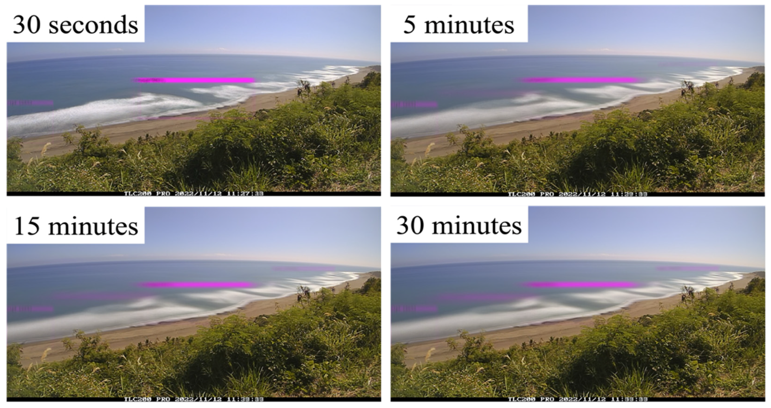
To investigate how different averaging times affect the resulting TIMEX images and what information these different images can provide, we established a fixed timelapse camera to monitor the southern section of the studied beach. The recorded videos were processed using an deep learning model to generate TIMEX images across multiple averaging durations. For rescue applications, the averaging times were set in seconds to allow for a rapid system response and timely warnings when rip currents emerge. Conversely, for persistence analysis, we employed extended averaging periods of 5, 15, and 30 min to examine the stability of the rip current channel. The results reveal that the rip current consistently appears in the same location across all time scales (Figure 12). As the averaging time increases from 30 s to 30 min, the water surface appears progressively smoother, making the features of the rip current more distinguishable from surrounding wave activity. The consistency of the rip current’s location across different time scales suggests a link between the rip current and fixed seabed features such as sandbar channels, which pose sustained hazards over time.

The short-term averaging approach is particularly relevant for immediate rescue operations. Our research framework employs a maximum averaging duration of 30 s to provide near-real-time hazard information. This timeframe aligns with the critical 20–60 s window during which a drowning victim typically struggles at the surface before succumbing to exhaustion [66]. During this period, the victim may attempt to call for help; however, this can quickly progress to silent drowning as their strength diminishes, rendering them unable to vocalize distress. By maintaining a short averaging period, lifeguards can receive timely alerts when intervention is still possible. This configuration allows the model to update rip status at high frequency under highly dynamic sea conditions, ensuring responsiveness without sacrificing accuracy. Moreover, the adjustable design allows the averaging duration to be extended, for example, to 5 or 10 min, during calmer sea states when rip current formation is less frequent.

For strategic beach management, long-term time-averaged images serve a fundamentally different purpose to immediate rescue applications. These images can be utilized by beach management authorities or lifeguards for risk assessment to determine whether to use red flags to prohibit swimming. However, many beaches around the world lack stationed lifeguards [8,67,68], and even where lifeguards are present, shortages often force a single individual to patrol large or multiple beach areas, as is common in places like Taiwan. Long-term time-averaged images provide an effective means to monitor wave behavior, rip currents, and surf conditions, capturing recurring patterns that enable continuous observation without constant human oversight. By allowing for the averaging duration to be extended beyond conventional 10 min intervals, long-lasting rip channels linked to sandbars or coastal structures, which often persist for days or weeks, can be revealed [69,70]. Consequently, beach management authorities can better detect shifts in rip current positions that would be invisible in shorter timeframes, enabling them to anticipate hazardous conditions more accurately, allocate their limited resources strategically to high-risk areas, and make informed decisions regarding swimming restrictions.

4.2. Latency Analysis and Deployment Consideration

The transition of the proposed AI framework from a laboratory to field deployment requires an evaluation of operational responsiveness. In this study, “latency” refers not only to hardware speed, but also to the need to balance rapid alert delivery with stable visuals for human verification. Consequently, the total time elapsed from video acquisition to the generation of a TIMEX image comprises computational latency and event confirmation latency. While the former is driven by hardware efficiency, the latter is a deliberate architectural choice designed to meet the requirements of professional coastal safety protocols.

4.2.1. Computational Latency

The computational latency is the time required for the hardware to process data once the analysis criteria are met.

• Model inference latency (~25 ms per frame): While the webcam records at 1080 × 1920 resolution, the video frames are resized to 416 × 416 for YOLOv4 inference. The detector operates at approximately 40 frames per second (FPS), corresponding to an inference time of about 25 ms per frame. Only frames with positive detections advance to further processing stages; therefore, the per-frame inference time does not directly determine the time to alert.
• Image registration (~230 ms per frame): For deployments involving pan-tilt-zoom (PTZ) cameras, this stage is the most intensive in computation. While this adds significant overhead, this step is bypassed in fixed-camera installations, drastically reducing the computational footprint.
• Image averaging (~5 ms per frame): This operation is highly efficient, introducing negligible latency compared to the registration stages.

Overall, each video frame can be processed efficiently, suggesting that the framework can handle continuous video streams in real time and operate on lightweight hardware platforms.

4.2.2. Event Confirmation Latency and Expert Validation Protocol

A defining characteristic of this framework is that the total time elapsed from initial video acquisition to the final TIMEX image is not a fixed hardware constant. Instead, it is a variable duration primarily governed by event confirmation latency. This latency represents the required duration over which detections must persist before further processing is triggered. It therefore defines the minimum and maximum bounds of the averaging period used to generate the TIMEX image. In addition, the length of the event confirmation latency is application-dependent and should be determined according to the operational objective of the system, particularly regarding which domain experts are responsible for validating the generated TIMEX images.

Building on this design principle, the event confirmation latency serves as the operational mechanism for implementing the expert validation protocol. This logical gate ensures that the system output aligns with the requirements of different stakeholders:

• On-site lifeguards or beach patrol: The logical gate is prioritized for rapid response. By setting the window to 8–30 s, the system will provide visual evidence within the critical 20–60 s window for drowning intervention
• Off-site officials: The logical gate can be adjusted to much wider ranges, for example, 5 to 10 min. It ensures that the resulting TIMEX image represents a stable, long-term hazard, providing the high statistical certainty required for administrative risk assessments and public safety updates.
• Off-site researchers: For long-term system maintenance, researchers examine accumulated TIMEX images occasionally. By reviewing these stabilized image reports, researchers can refine the model’s weights.

4.2.3. Deployment Considerations

In practical deployment, camera configuration is a primary determinant of system efficiency. Fixed webcams should be tilted to minimize sky coverage through horizon-based cropping, ensuring that the surf zone occupies most of the vertical field of view. Avoiding pan, tilt, or zoom motion eliminates the need for image registration and significantly reduces cumulative processing time. Input resolution should balance spatial detail and computational cost; resolutions between 1280 × 720 and 1920 × 1080 are generally sufficient to preserve rip channel morphology. A moderate sampling rate of around 2 frames per second generally captures the essential evolution of rip channels, while higher frame rates are better for rapidly changing conditions. For hardware, GPU resources should be utilized primarily for model inference, employing lightweight YOLO variants on edge devices like NVIDIA Jetson platforms. Meanwhile, the CPU can manage temporal averaging because it requires lower computational intensity. This approach leads to a balanced workload distribution across devices with moderate memory capacity.

5. Conclusions

In this study, an AI-based rip current warning system framework that integrates real-time object detection, adaptive time-averaged image generation, and expert verification is presented. Deep learning models trained on three different datasets were developed, and the results underscored the critical importance of training data selection and annotation methods. Models trained with more diverse and carefully labeled coastal imagery demonstrated greater robustness and accuracy in detecting rip currents, especially under complex conditions. Implementation of a pilot system using live webcam data from Jinzun Beach, Taiwan, confirmed the model’s robustness under varied lighting, camera, and wave conditions, as well as validated the framework’s practical viability. Moreover, the averaging times of the proposed framework can be adapted to address different operational needs. Short-term averaging could support rapid detection within the critical rescue window, while longer-term averaging may reveal persistent rip current channels associated with seabed morphology and inform broader risk assessment. This adaptability suggests potential for both real-time hazard alerts and longer-term pattern analysis, offering a basis for comprehensive coastal safety management tailored to specific beach conditions. Future work may explore recall oriented training strategies, such as cost sensitive or weighted loss formulations, to further reduce missed rip current detections in life safety contexts. Expanding the dataset to include more diverse and rare coastal conditions, potentially through generative approaches such as Generative Adversarial Networks (GAN) based data augmentation, and evaluating these strategies on state of the art YOLO versions could further enhance model robustness and deployment flexibility.

References

1. Houser, C.; Trimble, S.; Brander, R.; Brewster, B.C.; Dusek, G.; Jones, D.; Kuhn, J. Public Perceptions of a Rip Current Hazard Education Program: “Break the Grip of the Rip!”. Nat. Hazards Earth Syst. Sci. 2017, 17, 1003–1024. [Google Scholar] [CrossRef]
2. Lascody, R.L. East central florida rip current program. Natl. Weather Dig. 1998, 22, 25–30. [Google Scholar]
3. Brighton, B.; Sherker, S.; Brander, R.; Thompson, M.; Bradstreet, A. Rip Current Related Drowning Deaths and Rescues in Australia 2004–2011. Nat. Hazards Earth Syst. Sci. 2013, 13, 1069–1075. [Google Scholar] [CrossRef]
4. Withers, A.; Maldonado, S. On the Swimming Strategies to Escape a Rip Current: A Mathematical Approach. Nat. Hazards 2021, 108, 1449–1467. [Google Scholar] [CrossRef]
5. SLSA Surf Life Saving Australia National Coastal Safety Report 2023. 2023. Available online: https://issuu.com/surflifesavingaustralia/docs/ncsr23 (accessed on 25 February 2026).
6. Ishikawa, T.; Komine, T.; Aoki, S.I.; Okabe, T. Characteristics of Rip Current Drowning on the Shores of Japan. J. Coast. Res. 2014, 72, 44–49. [Google Scholar] [CrossRef]
7. Klein, A.H.d.F.; Santana, G.G.; Diehl, F.L.; de Menezes, J.T. Analysis of Hazards Associated with Sea Bathing: Results of Five Years Work in Oceanic Beaches of Santa Catarina State, Southern Brazil. J. Coast. Res. 2003, 107–116. Available online: https://www.jstor.org/stable/40928754 (accessed on 25 February 2026).
8. Hartmann, D. Drowning and Beach-Safety Management (BSM) along the Mediterranean Beaches of Israel—A Long-Term Perspective. J. Coast. Res. 2006, 22, 1505–1514. [Google Scholar] [CrossRef]
9. Scott, T.; Masselink, G.; Austin, M.J.; Russell, P. Controls on Macrotidal Rip Current Circulation and Hazard. Geomorphology 2014, 214, 198–215. [Google Scholar] [CrossRef]
10. Shin, C.H.; Noh, H.K.; Yoon, S.B.; Choi, J. Understanding of Rip Current Generation Mechanism at Haeundae Beach of Korea: Honeycomb Waves. J. Coast. Res. 2014, 72, 11–15. [Google Scholar] [CrossRef]
11. Gallop, S.L.; Bryan, K.R.; Pitman, S.J.; Ranasinghe, R.; Sandwell, D. Pulsations in Surf Zone Currents on a High Energy Mesotidal Beach in New Zealand. J. Coast. Res. 2016, 75, 378–382. [Google Scholar] [CrossRef]
12. Brander, R.W.; Bradstreet, A.; Sherker, S.; MacMahan, J. Responses of Swimmers Caught in Rip Currents: Perspectives on Mitigating the Global Rip Current Hazard. Int. J. Aquat. Res. Educ. 2011, 5, 11. [Google Scholar] [CrossRef][Green Version]
13. Johnson, D.; Stocker, R.; Head, R.; Imberger, J.; Pattiaratchi, C. A Compact, Low-Cost GPS Drifter for Use in the Oceanic Nearshore Zone, Lakes, and Estuaries. J. Atmos. Ocean. Technol. 2003, 20, 1880–1884. [Google Scholar] [CrossRef]
14. Austin, M.; Scott, T.; Brown, J.; Brown, J.; MacMahan, J.; Masselink, G.; Russell, P. Temporal Observations of Rip Current Circulation on a Macro-Tidal Beach. Cont. Shelf Res. 2010, 30, 1149–1165. [Google Scholar] [CrossRef]
15. Leatherman, S.; Leatherman, S. Techniques for Detecting and Measuring Rip Currents. Int. J. Earth Sci. Geophys. 2017, 3, 014. [Google Scholar] [CrossRef] [PubMed]
16. Trizna, D.B. Coherent Marine Radar Observations of Rip Current Features with High Temporal Resolution. In OCEANS 2018 MTS/IEEE Charleston; IEEE: Charleston, SC, USA, 2018; pp. 1–5. [Google Scholar]
17. Sridevi, T. Seasonal Variability of Rip Current Probability along a Wave-Dominated Coast Using High Resolution Satellites and Wave Data. J. Geomat. 2019, 13, 149–155. [Google Scholar]
18. Kumar, S.V.V.A.; Luhar, R.K.; Sharma, R.; Kumar, R. Design and Development of a Low-Cost GNSS Drifter for Rip Currents. Curr. Sci. 2020, 118, 273–279. [Google Scholar] [CrossRef]
19. Kim, H.D.; Kim, K.-H. Analysis of Rip Current Characteristics Using Dye Tracking Method. Atmosphere 2021, 12, 719. [Google Scholar] [CrossRef]
20. McGill, S.P.; Ellis, J.T. Rip Current and Channel Detection Using Surfcams and Optical Flow. Shore Beach 2022, 90, 50. [Google Scholar] [CrossRef]
21. Shimada, R.; Ishikawa, T.; Komine, T. Study of methods for detecting occurance of rip current using image analysis. Coast. Eng. Proc. 2023, 37, 13. [Google Scholar] [CrossRef]
22. Mori, I.; de Silva, A.; Dusek, G.; Davis, J.; Pang, A. Flow-Based Rip Current Detection and Visualization. IEEE Access 2022, 10, 6483–6495. [Google Scholar] [CrossRef]
23. De Silva, A.; Mori, I.; Dusek, G.; Davis, J.; Pang, A. Automated Rip Current Detection with Region Based Convolutional Neural Networks. Coast. Eng. 2021, 166, 103859. [Google Scholar] [CrossRef]
24. Zhu, D.; Qi, R.; Hu, P.; Su, Q.; Qin, X.; Li, Z. YOLO-Rip: A Modified Lightweight Network for Rip Currents Detection. Front. Mar. Sci. 2022, 9, 930478. [Google Scholar] [CrossRef]
25. Rashid, A.H.; Razzak, I.; Tanveer, M.; Robles-Kelly, A. RipDet: A Fast and Lightweight Deep Neural Network for Rip Currents Detection. In Proceedings of the 2021 International Joint Conference on Neural Networks (IJCNN), Virtual, 18–22 July 2021; IEEE: Shenzhen, China, 2021; pp. 1–6. [Google Scholar]
26. Khan, F.H.; Stewart, D.; de Silva, A.; Palinkas, A.; Dusek, G.; Davis, J.; Pang, A. RipScout: Realtime ML-Assisted Rip Current Detection and Automated Data Collection Using UAVs. IEEE J. Sel. Top. Appl. Earth Obs. Remote Sens. 2025, 18, 7742–7755. [Google Scholar] [CrossRef]
27. Rampal, N.; Shand, T.; Wooler, A.; Rautenbach, C. Interpretable Deep Learning Applied to Rip Current Detection and Localization. Remote Sens. 2022, 14, 6048. [Google Scholar] [CrossRef]
28. Brander, R.W.; MacMahan, J.H. Future Challenges for Rip Current Research and Outreach. In Rip Currents: Beach Safety, Physical Oceanography, and Wave Modeling; Leatherman, S., Fletemeyer, J., Eds.; CRC Press: Boca Raton, FL, USA, 2011; pp. 1–29. [Google Scholar]
29. Pitman, S.J.; Thompson, K.; Hart, D.E.; Moran, K.; Gallop, S.L.; Brander, R.W.; Wooler, A. Beachgoers’ Ability to Identify Rip Currents at a Beach in Situ. Nat. Hazards Earth Syst. Sci. 2021, 21, 115–128. [Google Scholar] [CrossRef]
30. Endo, S.; Shimada, R.; Ishikawa, T.; Komine, T. Can the Visualization of Rip Currents Prevent Drowning Accidents? Consideration of the Effect of Optimism Bias. Nat. Hazards 2022, 110, 2017–2033. [Google Scholar] [CrossRef]
31. Uebelhoer, L.; Koon, W.; Harley, M.D.; Lawes, J.C.; Brander, R.W. Characteristics and Beach Safety Knowledge of Beachgoers on Unpatrolled Surf Beaches in Australia. Nat. Hazards Earth Syst. Sci. 2022, 22, 909–926. [Google Scholar] [CrossRef]
32. Ballantyne, R.; Carr, N.; Hughes, K. Between the Flags: An Assessment of Domestic and International University Students’ Knowledge of Beach Safety in Australia. Tour. Manag. 2005, 26, 617–622. [Google Scholar] [CrossRef]
33. White, K.M.; Hyde, M.K. Swimming between the Flags: A Preliminary Exploration of the Influences on Australians’ Intentions to Swim between the Flags at Patrolled Beaches. Accid. Anal. Prev. 2010, 42, 1831–1838. [Google Scholar] [CrossRef]
34. Fletemeyer, J.R. Effectiveness of Panama City Beach Safety Program. In Rip Currents: Beach Safety, Physical Oceanography, and Wave Modeling; Leatherman, S., Fletemeyer, J., Eds.; CRC Press: Boca Raton, FL, USA, 2011; pp. 147–160. [Google Scholar]
35. Matthews, B.; Andronaco, R.; Adams, A. Warning Signs at Beaches: Do They Work? Saf. Sci. 2014, 62, 312–318. [Google Scholar] [CrossRef]
36. Basterretxea-Iribar, I.; Sotés, I.; Sanchez-Beaskoetxea, J.; Maruri, M.D.L.M. Beach Management Policy Analysis Concerning Safety Flag Systems in Northern Spain. Mar. Policy 2022, 144, 105226. [Google Scholar] [CrossRef]
37. Meir, A.; Hartmann, D.; Borowsky, A. Examining Lifeguards’ Abilities to Anticipate Surf Hazard Instigators—An Exploratory Study. Saf. Sci. 2021, 143, 105421. [Google Scholar] [CrossRef]
38. Bay, H.; Tuytelaars, T.; Van Gool, L. SURF: Speeded Up Robust Features. In European Conference on Computer Vision—ECCV 2006; Leonardis, A., Bischof, H., Pinz, A., Eds.; Springer: Berlin/Heidelberg, Germany, 2006; pp. 404–417. [Google Scholar]
39. Pianca, C.; Holman, R.; Siegle, E. Shoreline Variability from Days to Decades: Results of Long-Term Video Imaging. J. Geophys. Res. Oceans 2015, 120, 2159–2178. [Google Scholar] [CrossRef]
40. Qi, Z.-X.; Wang, H.-Z.; Wang, A.-J. Impacts of Dirty Data on Classification and Clustering Models: An Experimental Evaluation. J. Comput. Sci. Technol. 2021, 36, 806–821. [Google Scholar] [CrossRef]
41. Wu, D.Y.; Fang, Y.V.; Vo, D.T.; Spangler, A.; Seiler, S.J. Detailed Image Data Quality and Cleaning Practices for Artificial Intelligence Tools for Breast Cancer. JCO Clin. Cancer Inform. 2024, 8, e2300074. [Google Scholar] [CrossRef]
42. Mohan, A.; Kaseb, A.S.; Lu, Y.-H.; Hacker, T.J. Adaptive Resource Management for Analyzing Video Streams from Globally Distributed Network Cameras. IEEE Trans. Cloud Comput. 2021, 9, 40–53. [Google Scholar] [CrossRef]
43. Chen, P.-Y.; Chang, M.-C.; Hsieh, J.-W.; Chen, Y.-S. Parallel Residual Bi-Fusion Feature Pyramid Network for Accurate Single-Shot Object Detection. IEEE Trans. Image Process. 2021, 30, 9099–9111. [Google Scholar] [CrossRef]
44. Agarwal, S.; Terrail, J.O.D.; Jurie, F. Recent Advances in Object Detection in the Age of Deep Convolutional Neural Networks. arXiv 2018, arXiv:1809.03193. [Google Scholar]
45. Zaidi, S.S.A.; Ansari, M.S.; Aslam, A.; Kanwal, N.; Asghar, M.; Lee, B. A Survey of Modern Deep Learning Based Object Detection Models. Digit. Signal Process. 2022, 126, 103514. [Google Scholar] [CrossRef]
46. Sultana, F.; Sufian, A.; Dutta, P. A Review of Object Detection Models Based on Convolutional Neural Network. In Intelligent Computing: Image Processing Based Applications; Mandal, J.K., Banerjee, S., Eds.; Springer: Singapore, 2020; pp. 1–16. [Google Scholar]
47. Zou, Z.; Chen, K.; Shi, Z.; Guo, Y.; Ye, J. Object Detection in 20 Years: A Survey. Proc. IEEE 2023, 111, 257–276. [Google Scholar] [CrossRef]
48. Redmon, J.; Divvala, S.; Girshick, R.; Farhadi, A. You Only Look Once: Unified, Real-Time Object Detection. In Proceedings of the IEEE Conference on Computer Vision and Pattern Recognition, Las Vegas, NV, USA, 26 June–1 July 2016; pp. 779–788. [Google Scholar]
49. Wang, Z.; Zhu, W.; Zhao, W.; Xu, L. Balanced One-Stage Object Detection by Enhancing the Effect of Positive Samples. IEEE Trans. Circuits Syst. Video Technol. 2023, 33, 4011–4026. [Google Scholar] [CrossRef]
50. Hussain, M. YOLO-v5 Variant Selection Algorithm Coupled with Representative Augmentations for Modelling Production-Based Variance in Automated Lightweight Pallet Racking Inspection. Big Data Cogn. Comput. 2023, 7, 120. [Google Scholar] [CrossRef]
51. Park, M.-H.; Choi, J.-H.; Lee, W.-J. Object Detection for Various Types of Vessels Using the YOLO Algorithm. J. Adv. Mar. Eng. Technol. 2024, 48, 81–88. [Google Scholar] [CrossRef]
52. Bochkovskiy, A.; Wang, C.-Y.; Liao, H.-Y.M. YOLOv4: Optimal Speed and Accuracy of Object Detection. arXiv 2020, arXiv:2004.10934. [Google Scholar] [CrossRef]
53. Lestari, D.P.; Kosasih, R.; Handhika, T.; Murni; Sari, I.; Fahrurozi, A. Fire Hotspots Detection System on CCTV Videos Using You Only Look Once (YOLO) Method and Tiny YOLO Model for High Buildings Evacuation. In Proceedings of the 2019 2nd International Conference of Computer and Informatics Engineering (IC2IE), Banyuwangi, Indonesia, 10–11 September 2019; pp. 87–92. [Google Scholar]
54. Dewi, C.; Chen, R.-C.; Jiang, X.; Yu, H. Deep Convolutional Neural Network for Enhancing Traffic Sign Recognition Developed on Yolo V4. Multimed. Tools Appl. 2022, 81, 37821–37845. [Google Scholar] [CrossRef]
55. Jiang, C.; Ren, H.; Ye, X.; Zhu, J.; Zeng, H.; Nan, Y.; Sun, M.; Ren, X.; Huo, H. Object Detection from UAV Thermal Infrared Images and Videos Using YOLO Models. Int. J. Appl. Earth Obs. Geoinf. 2022, 112, 102912. [Google Scholar] [CrossRef]
56. Xu, C.; Wang, Z.; Du, R.; Li, Y.; Li, D.; Chen, Y.; Li, W.; Liu, C. A Method for Detecting Uneaten Feed Based on Improved YOLOv5. Comput. Electron. Agric. 2023, 212, 108101. [Google Scholar] [CrossRef]
57. Buckland, M.; Gey, F. The Relationship between Recall and Precision. J. Am. Soc. Inf. Sci. 1994, 45, 12–19. [Google Scholar] [CrossRef]
58. Christen, P.; Hand, D.J.; Kirielle, N. A Review of the F-Measure: Its History, Properties, Criticism, and Alternatives. ACM Comput. Surv. 2023, 56, 1–24. [Google Scholar] [CrossRef]
59. Grandini, M.; Bagli, E.; Visani, G. Metrics for Multi-Class Classification: An Overview. arXiv 2020, arXiv:2008.05756. [Google Scholar] [CrossRef]
60. Yu, J.; Zhang, W. Face Mask Wearing Detection Algorithm Based on Improved YOLO-V4. Sensors 2021, 21, 3263. [Google Scholar] [CrossRef] [PubMed]
61. Bogle, J.A.; Bryan, K.R.; Black, K.P.; Hume, T.M.; Healy, T.R. Video Observations of Rip Formation and Evolution. J. Coast. Res. 2001, 117–127. Available online: https://www.jstor.org/stable/25736280 (accessed on 25 February 2026).
62. Bruneau, N.; Castelle, B.; Bonneton, P.; Pedreros, R.; Almar, R.; Bonneton, N.; Bretel, P.; Parisot, J.-P.; Sénéchal, N. Field Observations of an Evolving Rip Current on a Meso-Macrotidal Well-Developed Inner Bar and Rip Morphology. Cont. Shelf Res. 2009, 29, 1650–1662. [Google Scholar] [CrossRef]
63. Trimble, S.; Penko, A. A Quantitative Evaluation of Rip Current Appearance in Argus Timex Imagery: When and Where Does Offshore Flow Correspond to Visible Features? In Proceedings of the Copernicus Meetings, Brussels, Belgium, 28 January 2020. [Google Scholar]
64. Zitová, B.; Flusser, J. Image Registration Methods: A Survey. Image Vis. Comput. 2003, 21, 977–1000. [Google Scholar] [CrossRef]
65. Rick Rip Currents. Available online: https://www.saltwater-dreaming.com/learn-to-surf/rip-currents.htm (accessed on 31 January 2024).
66. Tipton, M.; Montgomery, H. The Experience of Drowning. Med. Leg. J. 2022, 90, 17–26. [Google Scholar] [CrossRef]
67. Segura, L.E.; Arozarena, I.; Koon, W.; Gutiérrez, A. Coastal Drowning in Costa Rica: Incident Analysis and Comparisons between Costa Rican Nationals and Foreigners. Nat. Hazards 2022, 110, 1083–1095. [Google Scholar] [CrossRef]
68. Dehez, J.; Lyser, S. How Ocean Beach Recreational Quality Fits with Safety Issues? An Analysis of Risky Behaviours in France. J. Outdoor Recreat. Tour. 2024, 45, 100711. [Google Scholar] [CrossRef]
69. Dudkowska, A.; Boruń, A.; Malicki, J.; Schönhofer, J.; Gic-Grusza, G. Rip Currents in the Non-Tidal Surf Zone with Sandbars: Numerical Analysis versus Field Measurements. Oceanologia 2020, 62, 291–308. [Google Scholar] [CrossRef]
70. Houser, C.; Lehner, J.; Cherry, N.; Wernette, P. Machine Learning Analysis of Lifeguard Flag Decisions and Recorded Rescues. Nat. Hazards Earth Syst. Sci. 2019, 19, 2541–2549. [Google Scholar] [CrossRef]
Figure 1. Location of the study beach (Taitung City, Taiwan), study area (dashed line), and camera position (red pin; the green marker represents the study site, Jinzun, labeled in its local script.). Aerial view of Jinzun Beach.
Jmse 14 00496 g001
Figure 2. Conceptual framework of the rip current warning system.
Jmse 14 00496 g002
Figure 3. Illustration of dataset annotations and samples. (a) Samples from the NOAA and Refined-NOAA datasets, comparing original annotations (dark purple boxes) with refined annotations (yellow boxes) that incorporate adjacent beach areas for enhanced spatial context. The top row displays images with rip currents, while the bottom row shows images without. (b) Representative images from the BEACH dataset, showcasing diverse aerial and beach-level perspectives with rip currents labeled using axis-aligned bounding boxes (red boxes).
Jmse 14 00496 g003
Figure 4. SURF-based feature matching between two panning webcam images of the same beach. The left image serves as the reference frame. Matched keypoints are indicated by circles and connecting lines.
Jmse 14 00496 g004
Figure 5. The criterion for minimum separation. The arrow indicates the temporal progression.
Jmse 14 00496 g005
Figure 6. The criterion for maximum averaging frames. The arrow indicates the temporal progression.
Jmse 14 00496 g006
Figure 7. Comparison of NOAA, Refined-NOAA, and BEACH model predictions. (a) Successful detection by all models in a clear channel; (b) BEACH model outperformed the others by identifying three rip currents in a complex, small-scale scenario, highlighting the effectiveness of the refined labeling approach.
Jmse 14 00496 g007
Figure 8. Video recording intervals; gray boxes indicate webcam video, and red boxes indicate timelapse video. The blue curve indicates the normalized tidal height from 11 November to 13.
Jmse 14 00496 g008
Figure 9. Model inference results for Case A (northern beach perspective) and Case B (southern beach perspective). The bounding boxes indicate dark channel rip current patterns detected by the BEACH model. Representative frames are displayed in chronological order (top to bottom). The yellow “x” is the annotations added by the researcher to indicate the incorrect detections of the model.
Jmse 14 00496 g009
Figure 10. TIMEX results for the two video inference cases in Figure 9: (a) Case A and (b) Case B. Arrows indicate the rip current channels annotated by the researcher. Timestamp overlay blurred due to temporal averaging.
Jmse 14 00496 g010
Figure 11. Selection of TIMEX images resulting from our research: (a,g) zoomed-in TIMEX images of northern and southern sections; (b,c) northern, (d,e) central, and (f,h,i) southern sections within fixed fields of view (FOV). Subfigures correspond to rectangular regions in the panoramic image: northern (solid line), central (dash–dot line), and southern (dotted line). The red circle in (a) indicates a rip current channel; blurred content in (f) is a result of active camera rotation during the generation of TIMEX images. The yellow “x” is a researcher annotation marking incorrect model detections.
Jmse 14 00496 g011
Figure 12. The TIMEX images taken at various averaging times.
Jmse 14 00496 g012