Joint Arctic Sea Ice Forecasting Based on Graph-Structured Spatial Modeling and Temporal Transformers

Abstract

Rapid changes in Arctic sea ice exert significant impacts on regional climate feedbacks and high-latitude maritime activities, increasing the demand for accurate short-term forecasting of key sea ice variables. This study proposes a GraphTransformer-based framework for joint forecasting of sea ice thickness (SIT) and sea ice concentration (SIC), designed to address their strong spatiotemporal coupling under irregular Arctic Ocean geometries. A static spatial graph is constructed over effective Arctic marine grid cells, where neighborhood aggregation is applied at each time step to explicitly encode spatial correlations. A shared-parameter temporal Transformer is subsequently employed to model node-level long-range temporal dependencies and to perform direct multi-step forecasting. The model generates 14-day daily forecasts of SIT and SIC in a single forward pass. Experiments are conducted using multi-source daily data spanning from 1 January 2019 to 15 May 2025, with evaluation restricted to valid marine grid nodes. Results indicate that the proposed GraphTransformer achieves either the best or second-best performance among the compared models in multi-step forecasting accuracy. Ablation experiments further confirm the critical role of graph-based spatial encoding in enhancing spatial coherence and mitigating error propagation.

1. Introduction

Arctic sea ice is a fundamental component of the high-latitude climate system and plays a critical role in regulating sea ice–ocean–atmosphere interactions, controlling regional energy exchange, and modulating global climate feedback processes. Multi-source satellite observations and reanalysis datasets consistently demonstrate a pronounced long-term decline in both Arctic sea ice extent and thickness over recent decades. This decline has been widely recognized as a key manifestation of Arctic amplification under ongoing global warming [1,2]. The persistent alteration of sea ice conditions exerts substantial impacts on the Arctic climate structure and ecosystem stability. Moreover, it directly affects the safety and accessibility of high-latitude maritime activities. In particular, as Arctic shipping routes increasingly become seasonally navigable, the growing uncertainty associated with sea ice variability has emerged as a critical factor influencing navigation planning and operational risk assessment [3].

In characterizing Arctic sea ice conditions, sea ice concentration (SIC) and sea ice thickness (SIT) represent the two most fundamental physical variables [4]. SIC describes the horizontal distribution of sea ice and the variability of the ice edge, whereas SIT reflects the vertical structural properties of the ice cover and provides essential information for understanding thickness evolution and associated thermodynamic–dynamic processes [5,6]. Previous studies have demonstrated that these two variables are not independent during their formation and evolution. The spatial distribution of sea ice thickness constrains, to a certain extent, the stability and spatial extent of sea ice concentration [7]. Conversely, variations in sea ice concentration influence the thermodynamic and dynamic processes governing thickness evolution [8]. Therefore, conducting joint prediction of SIC and SIT within a unified modeling framework can enhance the physical consistency of sea ice representation and reduce structural biases arising from single-variable prediction.

Traditional Arctic sea ice prediction has primarily relied on coupled physical sea ice–ocean–atmosphere models. These models explicitly represent thermodynamic and dynamic processes and exhibit strong physical consistency in climate-scale simulations [9]. However, such models are typically computationally intensive and involve complex parameterizations. In high-temporal-resolution forecasting tasks, their performance is often sensitive to uncertainties in initial conditions and model parameters. With the continuous accumulation of multi-source remote sensing products and reanalysis datasets, data-driven approaches have gradually emerged as an important complementary direction in Arctic sea ice prediction research.

In recent years, deep learning methods have achieved substantial progress in Arctic sea ice prediction. Studies based on convolutional neural networks (CNNs) have demonstrated strong capability in extracting local spatial features of sea ice fields and have been applied to both SIC and SIT prediction tasks [10,11]. However, pure CNN architectures typically rely on fixed receptive fields for spatial modeling and are limited in explicitly capturing the temporal evolution of sea ice states. To incorporate temporal dependency, recurrent neural networks (RNNs) and their variants have been progressively introduced into sea ice forecasting research. Long short-term memory (LSTM) networks, in particular, have shown favorable performance in modeling temporal autocorrelation in sea ice time series [12]. Building upon this foundation, ConvLSTM integrates convolutional operations into the LSTM framework, enabling joint modeling of local spatial structures and temporal dynamics, and has become a widely adopted baseline in spatiotemporal sea ice prediction [13]. Furthermore, models such as PredRNN introduce spatiotemporal memory units to capture temporal dependencies at finer granularity, demonstrating enhanced capability in multi-step forecasting tasks [14].

Although CNN–RNN-based methods achieve joint modeling of spatial and temporal features to a certain extent, spatial dependencies are typically implicitly encoded through regular grid convolutions or sequential recurrence. Such representations are limited in explicitly characterizing the complex spatial topology of Arctic sea ice fields, which is shaped by irregular coastlines, land masking effects, and ocean dynamic processes.To address this limitation, graph-structured spatial modeling has gradually been introduced into Earth system prediction. By representing spatial grid cells as nodes and explicitly defining adjacency relationships among them, this framework enables more flexible representation of irregular spatial dependencies. Within this context, graph neural networks (GNNs) have been widely adopted to perform neighborhood information propagation and feature aggregation over graph structures [15] and have demonstrated effectiveness in modeling and predicting complex physical systems [16,17]. Furthermore, models such as GraphLSTM, which integrate graph neural networks with recurrent architectures, enable temporal modeling while preserving explicit spatial topological constraints, providing an alternative paradigm for Arctic sea ice prediction based on explicit spatial modeling [18].

Meanwhile, the self-attention mechanism has been introduced into Earth system modeling, and Transformer architectures have demonstrated strong capability in capturing long-range temporal dependencies. They have shown promising performance in various time-series forecasting and target detection tasks, often outperforming traditional recurrent models [19,20]. However, standard Transformer models do not explicitly incorporate spatial topological structures and are therefore limited in directly characterizing spatial adjacency constraints in Arctic sea ice fields. Consequently, integrating graph-structured spatial modeling with Transformer-based temporal modeling offers a promising approach for simultaneously enhancing spatial consistency and multi-step forecasting stability in the strongly coupled Arctic sea ice system.

Based on the above considerations, this study proposes a joint Arctic sea ice forecasting framework that integrates graph-structured spatial modeling with a temporal Transformer architecture, termed Joint Arctic Sea Ice Forecasting Based on GraphTransformer. In this framework, effective Arctic Ocean grid cells are represented as nodes in a static spatial graph, and spatial correlations of sea ice fields are explicitly encoded through graph neighborhood aggregation. On this basis, a temporal deep learning module is introduced to model node-level time series in a unified manner. Under a daily forecasting configuration, the model adopts a direct multi-step prediction strategy, simultaneously predicting daily sea ice thickness (SIT) and sea ice concentration (SIC) for the next 14 days in a single forward pass. This unified framework enables a more comprehensive representation of the spatiotemporal evolution of Arctic sea ice conditions.

2. Fundamental Theory

2.1. Spatiotemporal Characteristics of Arctic Sea Ice

Sea ice thickness (SIT) and sea ice concentration (SIC) exhibit pronounced spatiotemporal coupling characteristics in the Arctic system.

From a spatial perspective, sea ice states demonstrate strong correlations among neighboring grid cells. Thermodynamic and dynamic processes, such as heat exchange and wind-driven ice drift, facilitate information propagation across adjacent regions [10]. Meanwhile, the Arctic domain is characterized by irregular coastlines and a large proportion of invalid grid cells (e.g., land areas or persistently missing regions), which limit the capability of traditional regular-grid convolution-based methods in representing spatial relationships [18].

From a temporal perspective, sea ice variables exhibit strong temporal dependency and non-stationarity. Their evolution is influenced not only by short-term atmospheric forcing but also by seasonal oceanic variability [21]. Therefore, Arctic sea ice forecasting can be regarded as a high-dimensional, multivariate time-series problem with strong spatiotemporal coupling.

2.2. Graph-Structured Spatial Modeling

2.2.1. Graph Representation of Arctic Grid Cells

To characterize the spatial correlations of Arctic sea ice fields, the effective Arctic marine grid cells are represented as an undirected graph:

$$\mathcal{G}=(\mathcal{V},\mathcal{E})$$

(1)

where $\mathcal{V}=\{v_1,v_2,\dots ,v_N\}$ denotes the set of all valid marine grid nodes within the Arctic domain, and $\mathcal{E}$ represents the set of spatial adjacency relationships among nodes. This formulation follows the standard definition of graph structures in classical graph theory [22].

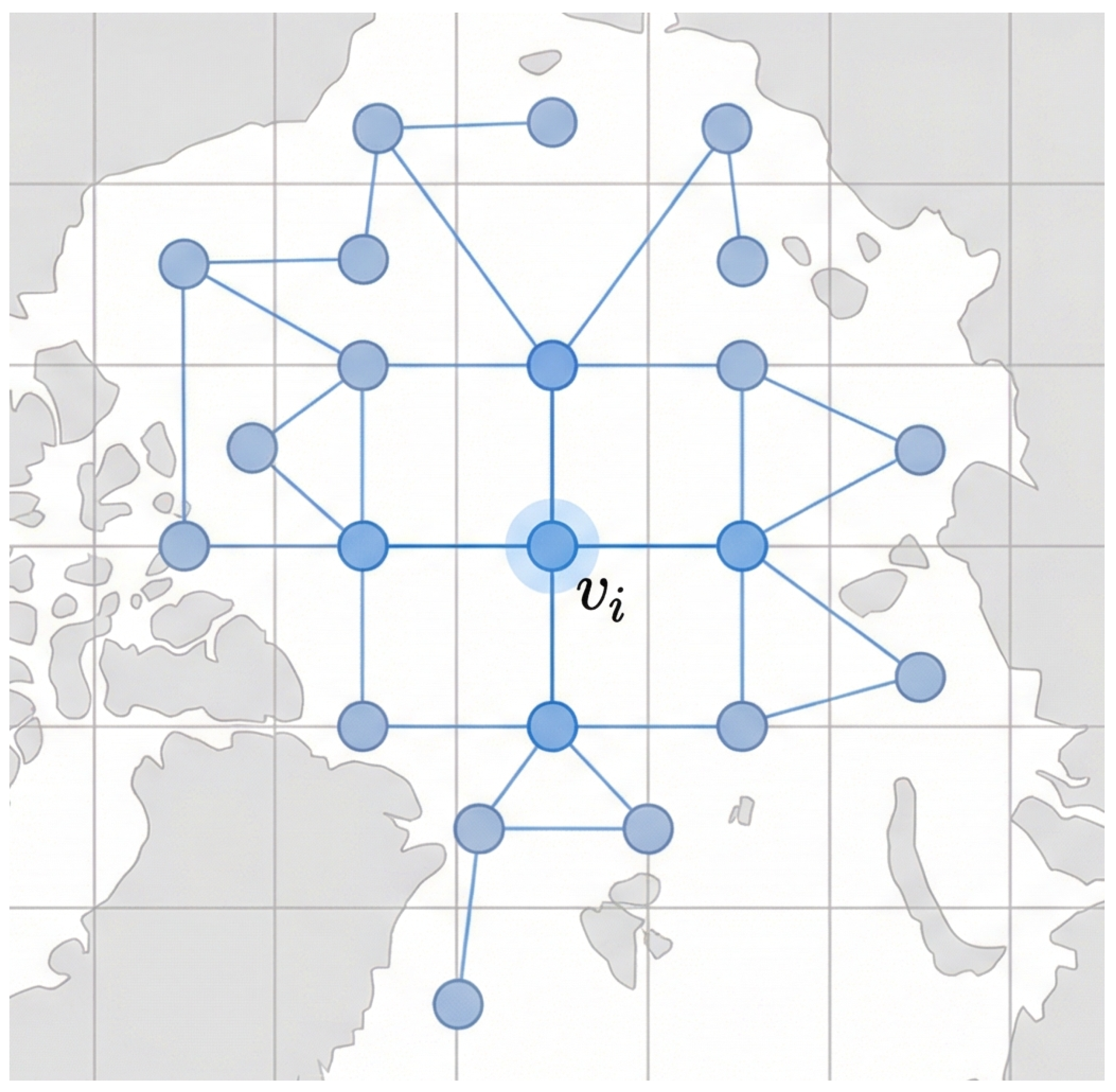
In this study, as illustrated in Figure 1, the spatial graph is constructed on a regular latitude–longitude grid using a four-neighbor connectivity scheme. Each node is connected exclusively to its immediately adjacent neighbors in the north, south, east, and west directions. Land areas and persistently invalid grid cells are excluded through spatial masking, such that the resulting graph comprises only valid Arctic marine nodes. The adjacency relationships remain fixed throughout the entire time series, thereby forming a static spatial graph.

It should be emphasized that the constructed graph encodes fixed geographical adjacency among marine grid cells rather than dynamic ice parcel trajectories. Although Arctic sea ice undergoes continuous advection and deformation under atmospheric and oceanic forcing, the adopted graph structure represents the underlying geographical topology of the discretized domain. In this study, all variables are defined on a regular latitude–longitude grid with a spatial resolution of $0.25°$ (approximately 25 km). Under this relatively fine spatial discretization and the short-term 14-day forecast horizon considered herein, the neighborhood relationships among adjacent marine grid cells remain topologically stable within the prediction window. Accordingly, the static graph serves as a structural spatial constraint that preserves local geographical connectivity, while the temporal evolution of sea ice drift and deformation is captured through the subsequent Transformer-based temporal modeling.

Figure 1 provides a schematic illustration of the four-neighbor connectivity for conceptual clarity. In practical implementation, each node corresponds to a single valid marine grid cell at the native $0.25°$ resolution, and adjacency relationships are strictly defined according to immediate north–south and east–west neighbors on the original grid. No additional spatial coarsening, interpolation, or resampling is introduced during graph construction.

2.2.2. Graph Neighborhood Aggregation

At time step t, the input feature vector of node i is defined as:

$${\mathbf{x}}_i^t\in {\mathbb{R}}^F$$

(2)

where F denotes the dimension of the input variables, including sea ice thickness (SIT), sea ice concentration (SIC), sea surface temperature (SST), near-surface air temperature (SAT), and 10 m wind components ($u10$, $v10$). The index i refers to a spatial node corresponding to a valid marine grid cell in the Arctic domain. The index t denotes the discrete daily time index (aligned with calendar dates).

To project the raw input features into a unified latent space, a linear transformation is first applied to obtain the initial node embedding at time step t:

$${\mathbf{h}}_i^{t,0}=W_0^{\left(g\right)}{\mathbf{x}}_i^t+{\mathbf{b}}_0^{\left(g\right)}$$

(3)

where ${\mathbf{h}}_i^{t,0}$ denotes the initial node representation before graph aggregation, $W_0\in {\mathbb{R}}^{d\times F}$ and ${\mathbf{b}}_0\in {\mathbb{R}}^d$ are learnable parameters, and d represents the hidden feature dimension.

Based on the static spatial adjacency constructed from the regular latitude–longitude grid, neighborhood information is aggregated using a mean aggregation scheme. For node i, the neighborhood message at time step t is computed as:

$${\mathbf{m}}_i^t={\displaystyle \frac{1}{\left|\mathcal{N}\right(i\left)\right|}}\sum _{j\in \mathcal{N}\left(i\right)}{\mathbf{h}}_j^{t,0}$$

(4)

where $\mathcal{N}\left(i\right)$ denotes the set of neighboring nodes of node i. This formulation is consistent with the mean aggregator proposed in GraphSAGE [23] and is widely used to capture local neighborhood effects.

The node representation is then updated by concatenating the self-embedding and aggregated neighborhood message, followed by a nonlinear transformation:

$${\tilde{\mathbf{h}}}_i^t=\sigma \left(W_1^{\left(g\right)}\left[h_i^{t,0}\Vert m_i^t\right]+{\mathbf{b}}_1^{\left(g\right)}\right)$$

(5)

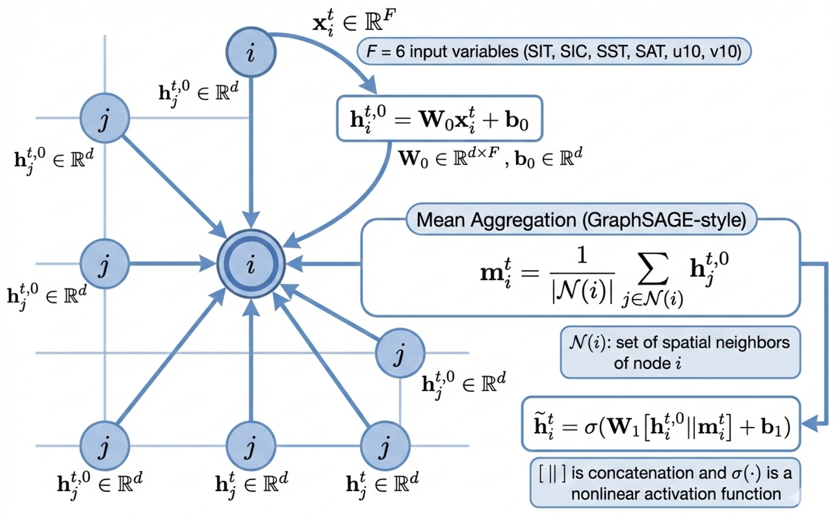
where $W_1^{\left(g\right)}$ and ${\mathbf{b}}_1^{\left(g\right)}$ are learnable parameters, $\sigma (·)$ denotes a nonlinear activation function, and ∥ represents feature concatenation. This operation effectively fuses self-node features and neighborhood information, producing spatially aware node representations for subsequent temporal modeling, as illustrated in Figure 2.

2.3. Temporal Modeling Based on Transformer

The Transformer leverages the self-attention mechanism to effectively capture dependencies among different time steps within a sequence. Unlike traditional recurrent neural networks, it does not rely on recursive structures but models temporal relationships entirely through attention mechanisms, thereby providing improved parallelization capability and stability in capturing long-range temporal dependencies [24].

2.3.1. Positional Encoding

Since the Transformer architecture contains neither recurrence nor convolution, it lacks inherent awareness of temporal order. To enable the model to distinguish the sequential relationships among time steps, positional encoding is incorporated into the input sequence.

For node i, the temporal feature sequence within a sliding time window is defined as:

$${\mathbf{S}}_i=\left[{\tilde{\mathbf{h}}}_i^{t-T+1},{\tilde{\mathbf{h}}}_i^{t-T+2},\dots ,{\tilde{\mathbf{h}}}_i^t\right]\in {\mathbb{R}}^{T\times d}$$

(6)

where T denotes the historical sequence length and $d=128$ represents the hidden feature dimension.

The positional encoding is constructed using sinusoidal functions, defined as:

$$PE(pos,2k)=\sin \left({\displaystyle \frac{pos}{{10000}^{2k/d}}}\right)$$

(7)

$$PE(pos,2k+1)=\cos \left({\displaystyle \frac{pos}{{10000}^{2k/d}}}\right)$$

(8)

where $pos$ denotes the temporal position index and k represents the feature dimension index.

The positional encoding is added element-wise to the input sequence representation, thereby embedding temporal order information into the sequence features.

2.3.2. Multi-Head Self-Attention

After positional encoding, the sequence representation is linearly projected to generate the query, key, and value matrices:

$$\mathbf{Q}={\mathbf{S}}_i{W}_Q$$

(9)

$$\mathbf{K}={\mathbf{S}}_i{W}_K$$

(10)

$$\mathbf{V}={\mathbf{S}}_i{W}_V$$

(11)

where ${\mathbf{S}}_i\in {\mathbb{R}}^{T\times d}$ denotes the input sequence representation, $W_Q,W_K\in {\mathbb{R}}^{d\times d_k}$ and $W_V\in {\mathbb{R}}^{d\times d_v}$ are learnable projection matrices. Accordingly, $\mathbf{Q},\mathbf{K}\in {\mathbb{R}}^{T\times d_k}$ and $\mathbf{V}\in {\mathbb{R}}^{T\times d_v}$ represent the query, key, and value matrices, respectively.

Self-attention is computed using the scaled dot-product formulation:

$$\mathrm{Attention}(\mathbf{Q},\mathbf{K},\mathbf{V})=\mathrm{softmax}\left({\displaystyle \frac{\mathbf{Q}{\mathbf{K}}^{\top }}{\sqrt{d_k}}}\right)\mathbf{V}$$

(12)

This mechanism calculates correlation weights among different time steps, enabling the modeling of temporal dependencies.

To enhance representational capacity, multi-head attention is employed:

$$\mathrm{MultiHead}(\mathbf{Q},\mathbf{K},\mathbf{V})=\mathrm{Concat}({\mathrm{head}}_1,\dots ,{\mathrm{head}}_h)W^O$$

(13)

$${\mathrm{head}}_i=\mathrm{Attention}(\mathbf{Q}{W}_i^Q,\mathbf{K}{W}_i^K,\mathbf{V}{W}_i^V)$$

(14)

where $W_i^Q,W_i^K\in {\mathbb{R}}^{d\times d_k}$, and $W_i^V\in {\mathbb{R}}^{d\times d_v}$ denote learnable projection matrices for the i-th attention head, and $W^O$ is the output projection matrix. In this work we employ $h=4$ parallel attention layers, or heads. For each of these we use $d_k=d_v=d/h=32$. The multi-head structure allows the model to learn multi-scale temporal dependencies in different representation subspaces.

2.3.3. Feed-Forward Network

Following the attention operation, each temporal position is independently transformed through a position-wise feed-forward network (FFN):

$$\mathrm{FFN}\left(\mathbf{x}\right)=\mathrm{ReLU}\left(W_1^{\left(f\right)}x+b_1^{\left(f\right)}\right)W_2^{\left(f\right)}+b_2^{\left(f\right)}$$

(15)

where $W_1^{\left(f\right)}$, $W_2^{\left(f\right)}$ and ${\mathbf{b}}_1^{\left(f\right)}$, ${\mathbf{b}}_2^{\left(f\right)}$ are learnable parameters. The FFN enhances nonlinear feature representation and improves the expressive capacity of the model.

3. Research Method

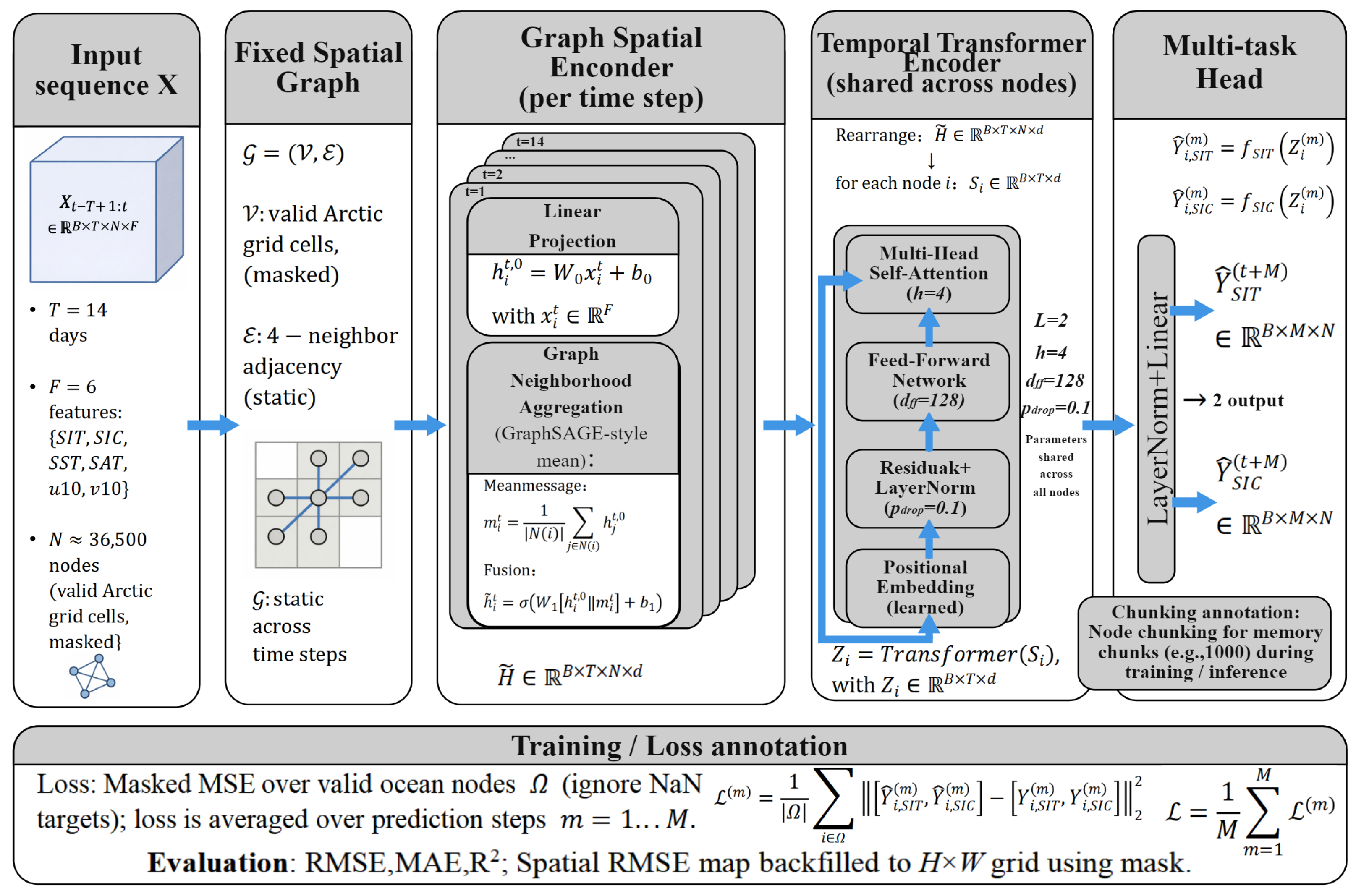
This section presents a graph-structured spatiotemporal forecasting framework for Arctic sea ice prediction, integrating graph-structured spatial modeling with a temporal Transformer encoder. The proposed method directly predicts future multi-step sea ice thickness (SIT) and sea ice concentration (SIC) over the horizon from $t+1$ to $t+14$.

The approach first constructs a static spatial graph over valid Arctic marine grid cells to characterize local spatial dependencies among sea ice variables and related meteorological factors. Subsequently, a temporal Transformer is introduced to model the temporal evolution of node-level features, enabling joint prediction across multiple time scales. The overall architecture is illustrated in Figure 3.

Under this framework, a direct multi-step forecasting strategy is adopted. The model generates predictions for $M=14$ future time steps in a single forward pass, rather than relying on recursive or rolling forecasting schemes. This design effectively mitigates the accumulation of temporal errors during multi-step prediction and allows the model to learn step-specific temporal characteristics within a unified forecasting framework [25,26].

During the evaluation stage, prediction metrics are computed independently for each forecast horizon m ($m=1,2,\dots ,14$) across all valid spatial nodes. The metrics are then averaged over all prediction steps to assess overall multi-step forecasting performance. This evaluation strategy is consistent with the multi-step loss aggregation scheme adopted during training, ensuring coherence between optimization objectives and evaluation criteria.

3.1. Overall Architecture

The Arctic sea ice system exhibits strong spatial correlations and temporal dependencies. Adjacent oceanic regions interact through thermodynamic exchange and dynamic transport processes, while the sea ice state at each grid cell demonstrates pronounced temporal continuity. To simultaneously capture these characteristics, the sea ice forecasting task is formulated as a spatiotemporal regression problem defined on a graph structure.

Assume that the Arctic domain contains N valid marine grid nodes. At each time step t, each node is associated with $F=6$ observational features. Given a historical observation sequence of length $T=14$, the model aims to jointly predict sea ice thickness (SIT) and sea ice concentration (SIC) over the next $M=14$ days (from $t+1$ to $t+14$):

$${\mathbf{Y}}_{t+1:t+M}=f\left({\mathbf{X}}_{t-T+1:t}\right)$$

(16)

where ${\mathbf{X}}_{t-T+1:t}$ denotes the historical multivariate spatiotemporal input sequence, and ${\mathbf{Y}}_{t+1:t+M}$ represents the joint multi-step predictions of SIT and SIC.

3.2. Graph-Structured Spatial Encoder

At each time step t, the model first applies a linear projection to the input features of all nodes, followed by neighborhood aggregation based on the static spatial graph. The parameters are shared across all time steps. The resulting spatially enhanced representation is:

$$\tilde{\mathbf{H}}\in {\mathbb{R}}^{B\times T\times N\times d}$$

(17)

where B denotes the batch size, T is the historical sequence length, N is the number of valid marine nodes, and d is the hidden feature dimension. The input feature dimension F corresponds to the variables SIT, SIC, SST, SAT, $u10$, and $v10$.

This graph-structured spatial encoding explicitly injects spatial structural information before temporal modeling.

3.3. Temporal Transformer Encoder

After spatial encoding, temporal modeling is performed independently for each spatial node. The graph-enhanced feature tensor is reorganized along the node dimension. For node i, the temporal sequence representation is:

$${\mathbf{S}}_i\in {\mathbb{R}}^{B\times T\times d}$$

(18)

A shared-parameter temporal Transformer encoder is then applied to model the evolution dynamics across all nodes:

$${\mathbf{Z}}_i=\mathrm{Transformer}\left({\mathbf{S}}_i\right)$$

(19)

The temporal Transformer effectively captures long-range dependencies and nonlinear evolution patterns along the temporal dimension.

3.4. Multi-Task Prediction and Loss Function

To jointly predict sea ice thickness (SIT) and sea ice concentration (SIC), a shared encoder with task-specific prediction heads is designed on top of the Transformer outputs [27]. The final temporal representations are linearly projected to generate task-specific forecasts:

$${\widehat{Y}}_{i,\mathrm{SIT}}^{\left(m\right)}=\mathrm{ReLU}\left(f_{\mathrm{SIT}}\left({\mathbf{Z}}_i^{\left(m\right)}\right)\right)$$

(20)

$${\widehat{Y}}_{i,\mathrm{SIC}}^{\left(m\right)}=\mathrm{Sigmoid}\left(f_{\mathrm{SIC}}\left({\mathbf{Z}}_i^{\left(m\right)}\right)\right)$$

(21)

where ${\mathbf{Z}}_i^{\left(m\right)}$ denotes the hidden representation of node i corresponding to forecast step m, and $f_{\mathrm{SIT}}(·)$ and $f_{\mathrm{SIC}}(·)$ represent task-specific linear mappings. The ReLU activation enforces non-negativity of the SIT forecasts such that ${\widehat{Y}}_{i,\mathrm{SIT}}^{\left(m\right)}\ge 0$, while the Sigmoid activation constrains the SIC forecasts within the physically admissible interval ${\widehat{Y}}_{i,\mathrm{SIC}}^{\left(m\right)}\in [0,1]$. These physically informed output transformations are applied consistently during both training and inference, thereby ensuring that all forecasts remain physically meaningful and numerically stable.

Considering the presence of invalid grid cells in the Arctic domain, loss computation is restricted to the set of valid marine nodes. Let $\mathrm{\Omega }$ denote the set of nodes with valid SIT and SIC observations [28]. For each forecast horizon m ($m=1,\dots ,M$), the multi-task regression loss is defined as:

$$L^{\left(m\right)}={\displaystyle \frac{1}{\left|\mathrm{\Omega }\right|}}\sum _{i\in \mathrm{\Omega }}{∥\left[{\widehat{Y}}_{i,\mathrm{SIT}}^{\left(m\right)},{\widehat{Y}}_{i,\mathrm{SIC}}^{\left(m\right)}\right]-\left[Y_{i,\mathrm{SIT}}^{\left(m\right)},Y_{i,\mathrm{SIC}}^{\left(m\right)}\right]∥}_2^2$$

(22)

The final training objective is obtained by averaging the losses across all forecast steps:

$$L={\displaystyle \frac{1}{M}}\sum _{m=1}^M{L}^{\left(m\right)}$$

(23)

3.5. Evaluation Metrics

To quantitatively assess model performance in Arctic sea ice forecasting, three evaluation metrics are employed: root mean square error (${\mathrm{RMSE}}_m$), mean absolute error (${\mathrm{MAE}}_m$), and coefficient of determination ($R_m^2$) [21]. All metrics are computed exclusively over the valid marine node set $\mathrm{\Omega }$ to avoid the influence of land and missing regions [28].

For each forecast horizon m ($m=1,2,\dots ,14$), the RMSE is defined as:

$${\mathrm{RMSE}}_m=\sqrt{{\displaystyle \frac{1}{\left|\mathrm{\Omega }\right|}}\sum _{i\in \mathrm{\Omega }}{\left({\widehat{Y}}_i^{t+m}-Y_i^{t+m}\right)}^2}$$

(24)

where ${\widehat{Y}}_i^{t+m}$ and $Y_i^{t+m}$ denote the predicted and observed values at time step $t+m$ for node i, respectively.

The mean absolute error (MAE) is defined as:

$${\mathrm{MAE}}_m={\displaystyle \frac{1}{\left|\mathrm{\Omega }\right|}}\sum _{i\in \mathrm{\Omega }}\left|{\widehat{Y}}_i^{t+m}-Y_i^{t+m}\right|$$

(25)

The coefficient of determination is defined as:

$$R_m^2=1-{\displaystyle \frac{{\sum }_{i\in \mathrm{\Omega }}{\left({\widehat{Y}}_i^{t+m}-Y_i^{t+m}\right)}^2}{{\sum }_{i\in \mathrm{\Omega }}{\left(Y_i^{t+m}-{\overline{Y}}^{t+m}\right)}^2}}$$

(26)

$${\overline{Y}}^{t+m}={\displaystyle \frac{1}{\left|\mathrm{\Omega }\right|}}\sum _{i\in \mathrm{\Omega }}{Y}_i^{t+m}$$

(27)

To evaluate overall performance under the direct multi-step forecasting setting, the metrics are averaged across all forecast horizons:

$$\overline{\mathrm{RMSE}}={\displaystyle \frac{1}{M}}\sum _{m=1}^M{\mathrm{RMSE}}_m$$

(28)

$$\overline{\mathrm{MAE}}={\displaystyle \frac{1}{M}}\sum _{m=1}^M{\mathrm{MAE}}_m$$

(29)

$$\overline{R^2}={\displaystyle \frac{1}{M}}\sum _{m=1}^M{R}_m^2$$

(30)

where $\overline{\mathrm{RMSE}}$ denotes the average root mean square error over the 14 forecast days, $\overline{\mathrm{MAE}}$ denotes the average mean absolute error over the 14 forecast days, and $\overline{R^2}$ represents the averaged coefficient of determination.

4. Experimental Validation and Analysis

The experiments were conducted on a workstation equipped with a 13th Gen Intel^® Core™ i7-13620H CPU, 16 GB RAM, and an NVIDIA GeForce RTX 4060 Laptop GPU for accelerated deep learning training and inference. An NVMe solid-state drive (SSD) was used to ensure efficient read/write performance for large-scale spatiotemporal and grid-based datasets.

The software environment was configured with Windows 10 and the PyTorch (version 2.8.0) deep learning framework, with CUDA acceleration enabled. All model training and evaluation procedures were performed on the GPU.

To address the large number of spatial grid nodes in the Arctic domain, a node-wise partitioning strategy was adopted during both training and inference to reduce GPU memory consumption and improve computational efficiency. This design ensures stable model execution under limited hardware resources [29].

4.1. Data Description

This study describes the datasets and their spatiotemporal characteristics used in the experiments. The forecasting samples are constructed from multi-year daily Arctic sea ice and atmospheric reanalysis data spanning from 1 January 2019 to 15 May 2025. The prediction targets are sea ice thickness (SIT) and sea ice concentration (SIC). The input features include sea ice state variables (SIT and SIC) as well as key meteorological drivers, namely sea surface temperature (SST), near-surface air temperature (SAT), and 10 m wind components ($u10$, $v10$), to characterize the combined thermodynamic and dynamic influences on sea ice evolution.

The SIT and SIC data are obtained from products released by the National Snow and Ice Data Center (NSIDC). The meteorological variables (SST, SAT, $u10$, $v10$) are derived from the ERA5 reanalysis dataset provided by the European Centre for Medium-Range Weather Forecasts (ECMWF) on behalf of the Copernicus Climate Change Service (C3S) [30].

All variables are regridded to a unified regular latitude–longitude grid with a spatial resolution of approximately 0.25° (about 25 km) [31]. This spatial resolution is selected to remain consistent with the native resolution of the ERA5 reanalysis data and to preserve the spatial detail of the original sea ice products without additional coarsening. At this resolution, land areas and persistently invalid grid cells are removed through spatial masking, retaining only valid Arctic marine regions for modeling. Each valid grid cell is treated as a node in the graph structure, resulting in approximately $N\approx \mathrm{36,500}$ spatial nodes. A four-neighbor connectivity scheme is adopted to construct the spatial graph, which remains fixed throughout the entire time series, forming a static spatial graph.

In the temporal modeling configuration, a direct multi-step forecasting strategy is adopted. Given a historical observation window of $T=14$ days, the model generates predictions for the next $M=14$ days (from $t+1$ to $t+14$) in a single forward pass. The dataset was partitioned sequentially into training, validation, and test sets in chronological order to preserve temporal causality and prevent information leakage, as summarized in

Table 1. Temporal partitioning of the dataset used for model development and evaluation.

Subset	Time Period	Duration
Training	1 Jan. 2019 to 31 Dec. 2022	4 years
Validation	1 Jan. 2023 to 30 Sep. 2024	21 months
Test	1 Oct. 2024 to 15 May 2025	7.5 months

.

4.2. Data Preprocessing

To ensure consistency across multiple data sources in both spatial and temporal dimensions and to improve training stability and prediction reliability, systematic preprocessing is applied prior to model training. The main steps are as follows:

(1) Regridding and Spatial Alignment. SIT, SIC, and ERA5 meteorological variables are regridded onto a unified latitude–longitude grid to ensure pointwise spatial correspondence across variables [32].

(2) Spatial Masking and Invalid Node Handling. Land regions and persistently invalid grid cells are removed through spatial masking. Subsequent modeling and evaluation are performed exclusively on valid Arctic marine nodes.

(3) Missing Value Processing. Missing values in input features are uniformly filled with zeros. For supervised targets, masked exclusion is applied such that missing labels do not contribute to loss computation, thereby reducing the influence of noisy targets [28].

(4) Standardization. Each input variable is independently standardized. The normalization parameters are computed solely from the training set and consistently applied to the validation and test sets to prevent information leakage.

4.3. Hyperparameter Selection

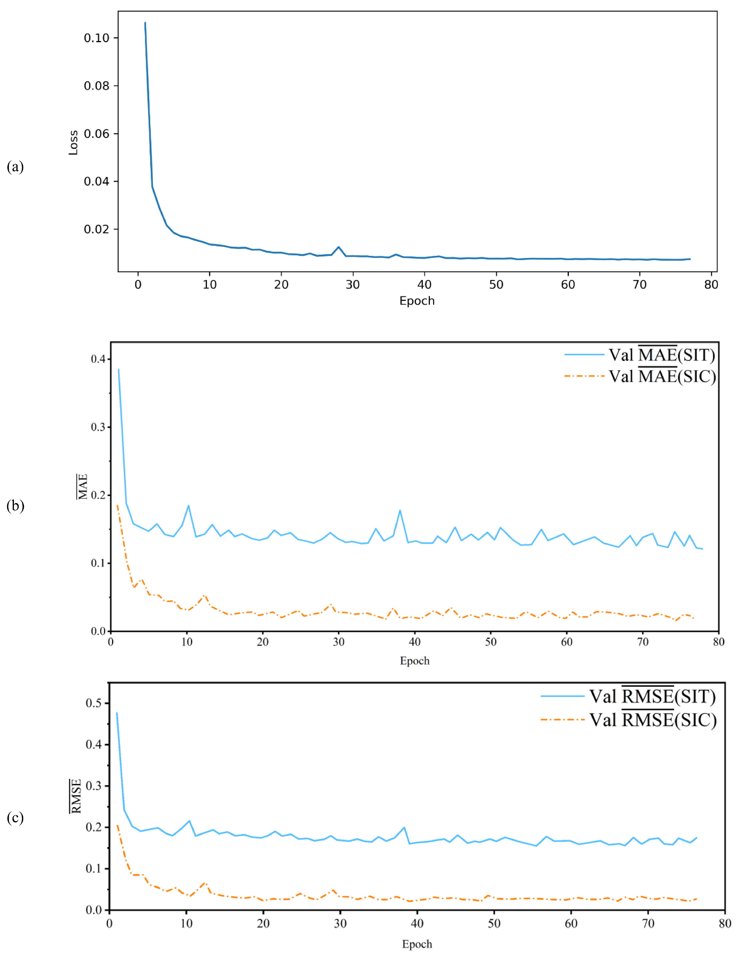
During model training, hyperparameters were selected based on validation performance. As shown in Figure 4a, the training loss of the proposed GraphTransformer model decreases rapidly from approximately 0.105 to below 0.02 within the first 10 epochs, followed by gradual stabilization. Between epochs 50 and 77, the loss remains stable around 0.010, indicating sufficient convergence.

According to the validation error curves (Figure 4b,c), at the selected 77th epoch, the model achieves a 14-day averaged performance of $\overline{\mathrm{MAE}}\approx 0.1531\mathrm{m}$ and $\overline{\mathrm{RMSE}}\approx 0.2252\mathrm{m}$ for sea ice thickness (SIT), with $\overline{R^2}>0.86$. For sea ice concentration (SIC), the validation results show $\overline{\mathrm{MAE}}\approx 0.0457$, $\overline{\mathrm{RMSE}}\approx 0.1079$, and $\overline{R^2}\approx 0.95$.

In the later training stage, no sustained metric degradation or significant oscillations are observed. The training and validation trends remain consistent, and no evident overfitting is detected.

Considering both convergence behavior and validation accuracy, the model parameters at epoch 77 are selected as the final configuration for subsequent quantitative evaluation and comparative analysis on the test set.

4.4. Spatial Prediction Results of the GraphTransformer Model

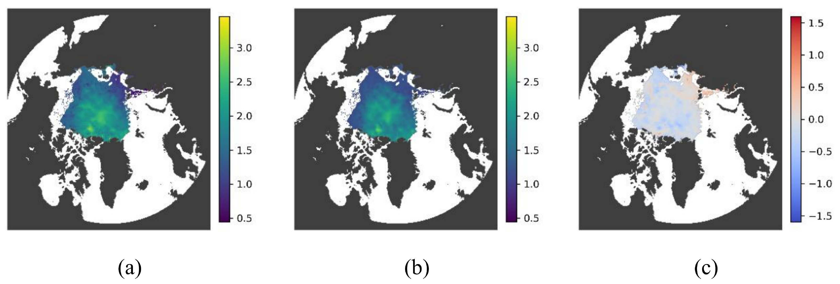
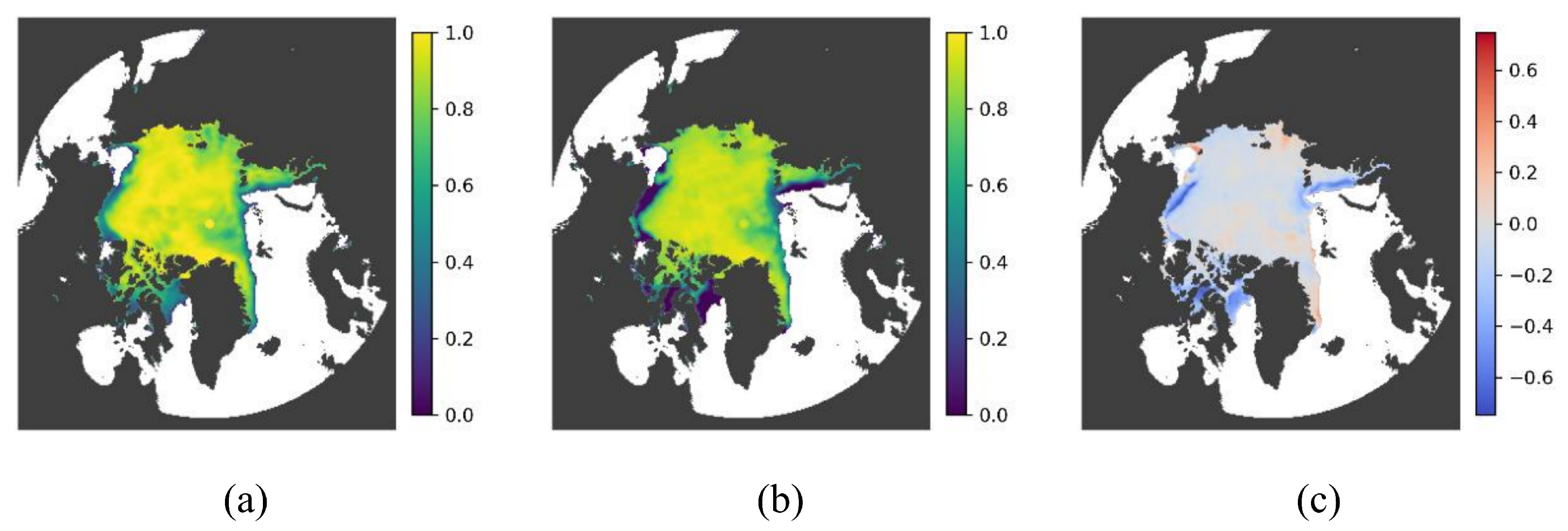
To visually assess the spatial modeling capability of the proposed GraphTransformer in Arctic sea-ice forecasting, we select a representative test-case period from 3 November 2024 to 16 November 2024. The spatial prediction performance is evaluated for sea ice thickness (SIT) and sea ice concentration (SIC). Figure 5 and Figure 6 present the 14-day mean spatial fields over this period, including the ground-truth field, the GraphTransformer prediction, and the corresponding error field.

For SIT prediction (Figure 5), the GraphTransformer model effectively reconstructs the high-thickness distribution over the central Arctic multi-year ice region. The predicted field exhibits strong agreement with the ground-truth field in terms of overall spatial pattern, spatial extent, and the location of high-value regions (Figure 5a,b). The corresponding error field indicates that prediction errors remain relatively small across most areas, with larger discrepancies primarily concentrated along the sea-ice edge transition zones (Figure 5c). This suggests that, while fine-scale characterization of ice-edge dynamics remains challenging, the model achieves strong overall spatial consistency in SIT prediction.

For SIC prediction (Figure 6), the model demonstrates similarly robust spatial fitting capability. The spatial structure of high-concentration continuous ice regions is accurately reproduced (Figure 6a,b), while the error field remains close to zero over the majority of the Arctic domain, with localized deviations mainly appearing in fragmented ice-edge regions (Figure 6c). Overall, these results indicate that the graph-structured spatial modeling explicitly introduces neighborhood constraints, enabling the model to preserve spatial continuity under large-scale Arctic spatial topology and to suppress the uncontrolled propagation of prediction errors in regions characterized by high uncertainty, such as ice margins.

4.5. Physical Consistency Analysis Between Predicted SIT and SIC

To evaluate whether the model outputs satisfy fundamental physical constraints, a physical consistency analysis was conducted on the GraphTransformer predictions of sea ice thickness (SIT) and sea ice concentration (SIC) over the test set. Based on the physical framework of sea ice thickness distribution theory, SIC quantifies the fractional ice-covered area within a grid cell [33]. When SIC approaches zero, indicating open-water conditions, the corresponding SIT is physically expected to approach zero as well. Therefore, cases in which low SIC coincides with appreciable SIT are considered physically inconsistent.

The physical inconsistency criterion is defined as

$${\mathrm{SIC}}_{\mathrm{pred}}<0.01\mathrm{and}{\mathrm{SIT}}_{\mathrm{pred}}>0.05\mathrm{m}.$$

(31)

where $\mathrm{SIC}=0.01$ approximates the open-water threshold, and $\mathrm{SIT}=0.05\mathrm{m}$ represents the lower bound of detectable ice thickness.

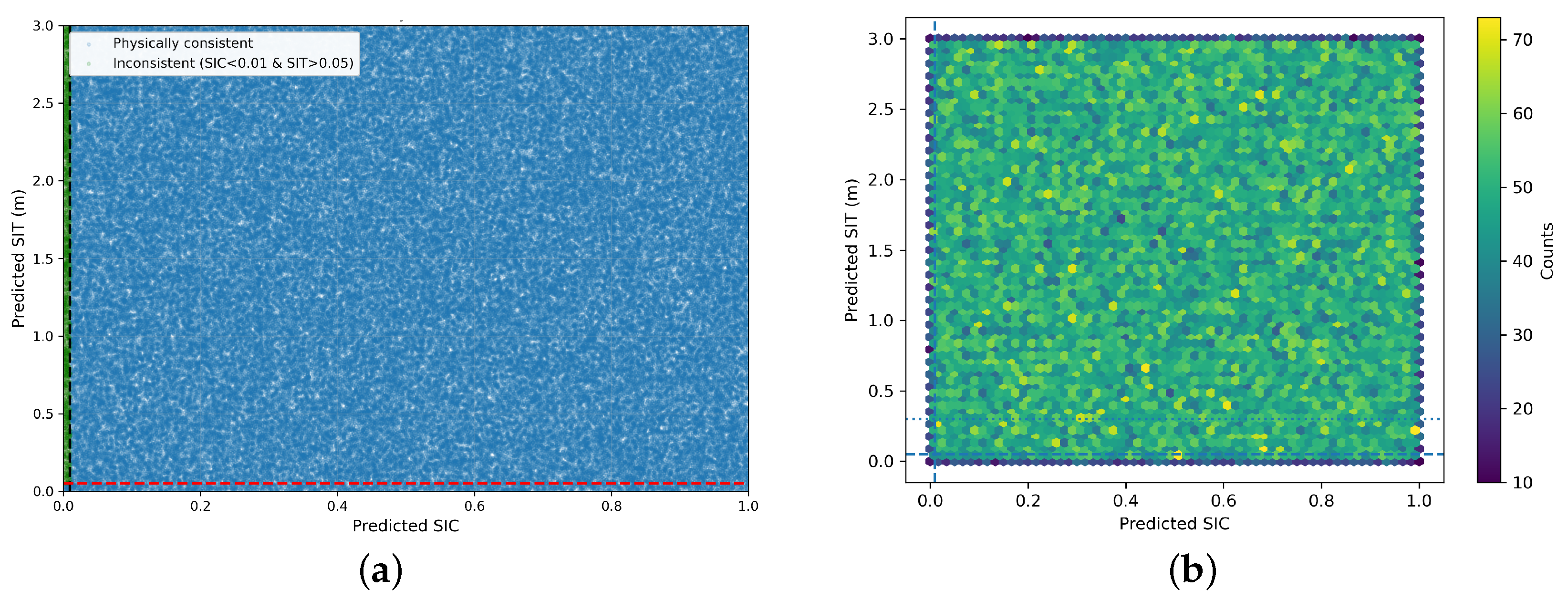
Figure 7a presents the scatter distribution of predicted SIC versus predicted SIT across all valid spatial nodes and all forecast lead times in the test set. The horizontal axis denotes predicted SIC, and the vertical axis denotes predicted SIT. The black dashed vertical line indicates the SIC threshold of 0.01, while the red dashed horizontal line represents the SIT threshold of 0.05 m. The upper-left region (SIC $<0.01$ and SIT $>0.05$ m) corresponds to physically inconsistent predictions. Statistical results show that this region accounts for only 0.98% of all samples, indicating that such violations occur infrequently. The vast majority of predictions fall within physically reasonable regions, suggesting that the model satisfies fundamental physical consistency in a statistical sense.

To further examine the joint distribution structure, Figure 7b presents a two-dimensional hexagonal bin density map (hexbin) of predicted SIT and SIC. The color intensity represents the sample count within each bin. No significant high-density accumulation is observed in the physically inconsistent region, indicating the absence of systematic physical violations. The overall joint distribution exhibits a continuous and stable structure without anomalous clustering of large SIT values under near-zero SIC conditions.

It should be noted that this analysis aggregates all valid spatial nodes and all forecast lead times in the test set (flattened over space and lead times). Therefore, the reported results reflect overall statistical physical consistency rather than behavior at a specific time step or localized region. Combined evidence from the scatter distribution and density map demonstrates that the GraphTransformer maintains the fundamental physical relationship between SIT and SIC while achieving accurate multi-step forecasts.

4.6. Comparative Analysis of Different Models

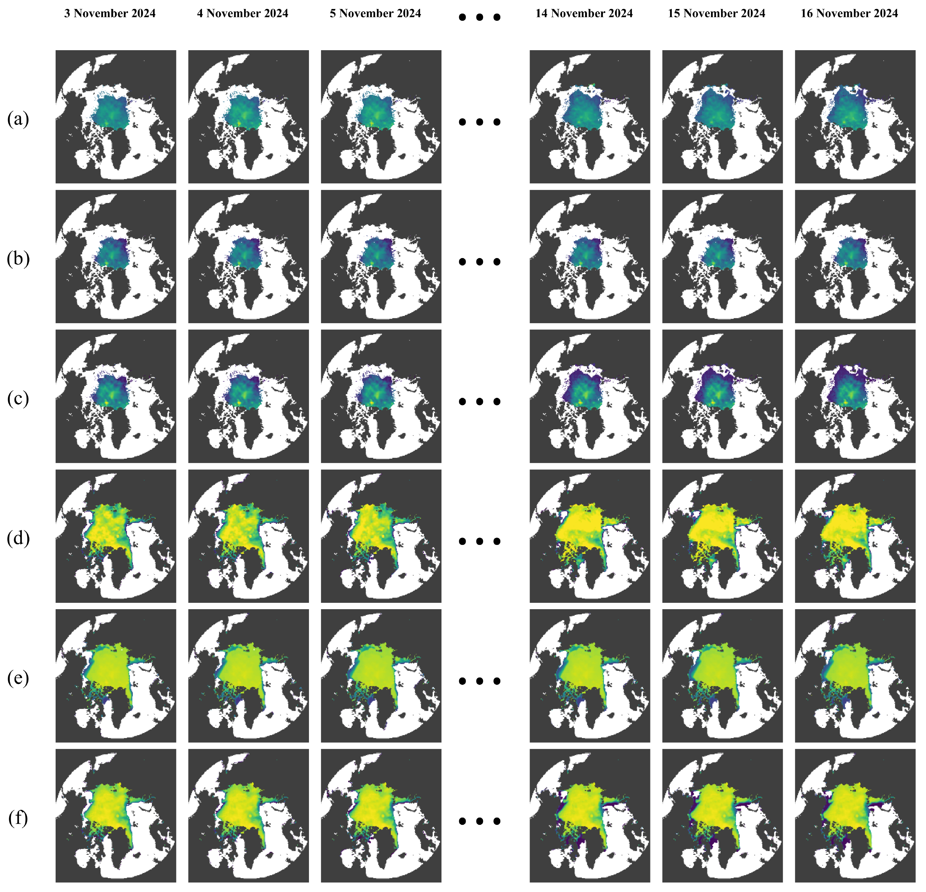
To comprehensively evaluate the effectiveness of the proposed framework, ConvLSTM, GraphLSTM, PredRNN, and U-Net are selected as baseline models. All methods are implemented under the same dataset and experimental settings, and comparative analysis is conducted using the test samples from 3 November 2024 to 16 November 2024.

4.6.1. Spatial Distribution Analysis of Sea Ice Thickness (SIT)

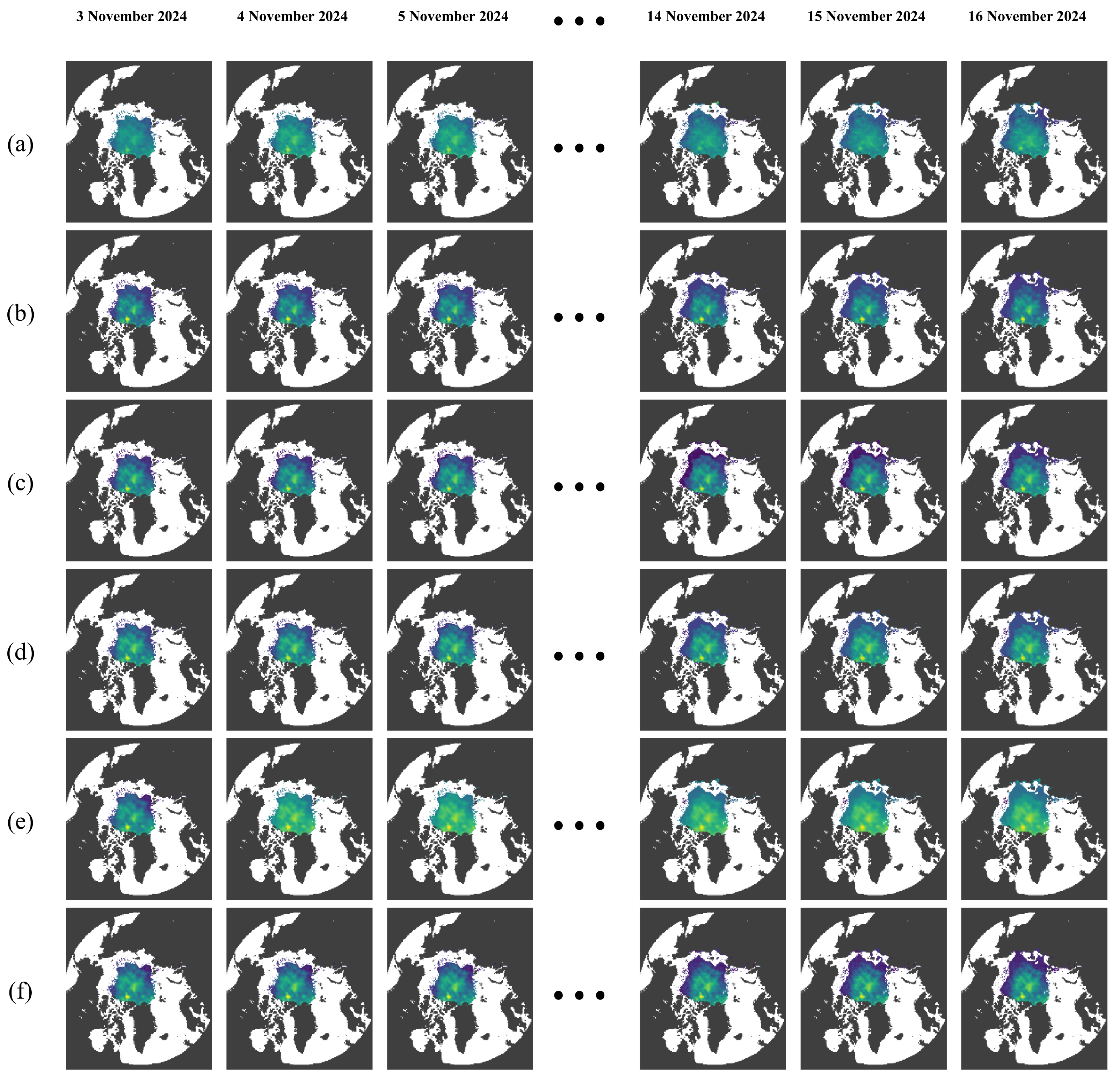
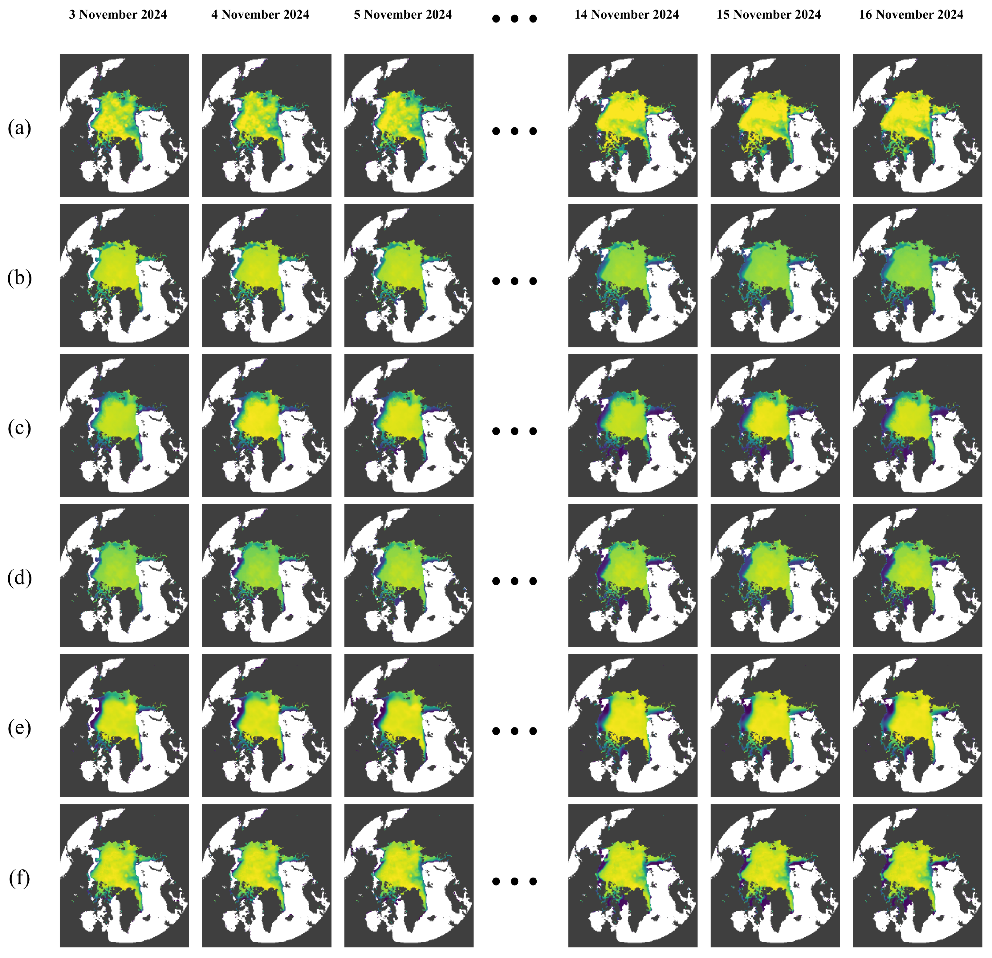
Figure 8 presents the spatiotemporal prediction results of SIT during the test period for all models. ConvLSTM, GraphLSTM, and PredRNN generally capture the large-scale outline of the ice-covered region; however, they exhibit varying degrees of spatial blurring in high-thickness areas, particularly in terms of structural continuity and fine-scale details. U-Net improves local feature representation to some extent, yet its overall spatial consistency remains limited.

In contrast, the proposed GraphTransformer better preserves the overall morphology of the ice-covered region while maintaining enhanced spatial integrity and continuity in high-thickness zones (Figure 8f). These results demonstrate the advantage of graph-structured spatial modeling combined with temporal attention mechanisms in capturing both large-scale spatial topology and fine-grained structural information.

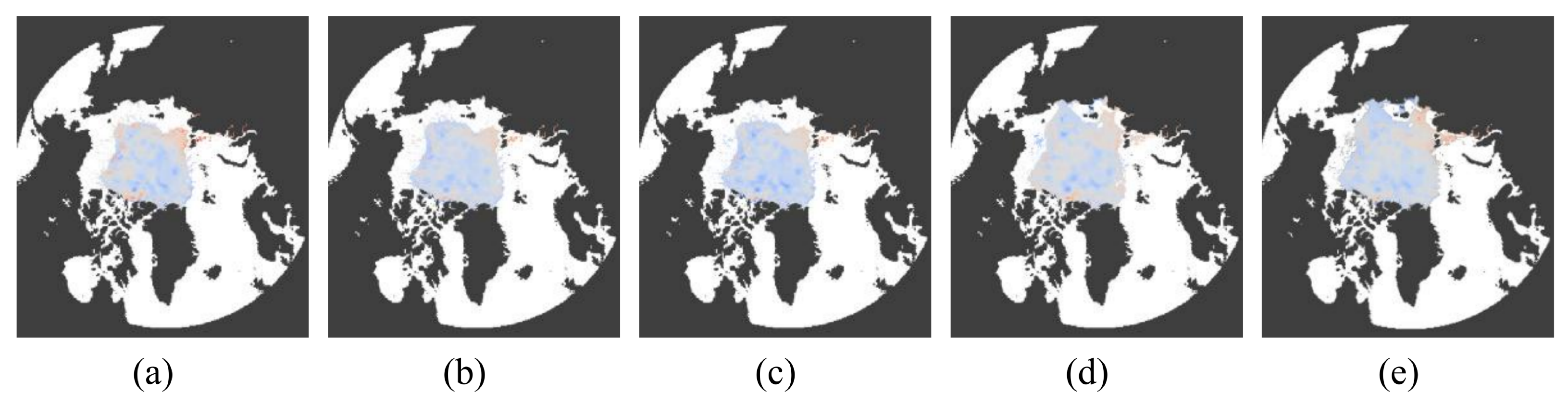
Figure 9 illustrates the spatial distribution of the 14-day mean prediction errors of sea ice thickness (SIT) for different models during the test period (3 November 2024 to 16 November 2024).

Compared with the baseline models, the proposed GraphTransformer exhibits the smallest overall error magnitude and a more spatially homogeneous error distribution (Figure 9e). This indicates improved spatial prediction accuracy and enhanced stability relative to the competing approaches.

4.6.2. Spatial Distribution Comparison of Sea Ice Concentration (SIC)

Figure 10 presents the spatiotemporal prediction results of different models for the sea ice concentration (SIC) forecasting task. Overall, all models are capable of capturing the primary high-concentration ice regions. However, noticeable differences emerge in the marginal ice zone and low-concentration areas.

ConvLSTM, GraphLSTM, and PredRNN tend to exhibit localized overestimation or underestimation in fragmented ice-edge regions, indicating limited capability in resolving fine-scale spatial variability. U-Net shows improved local detail representation but demonstrates over-smoothing effects along the ice edge and in low-concentration regions.

In contrast, the proposed GraphTransformer more accurately reconstructs the spatial morphology of sea ice concentration and preserves smoother and more physically consistent transition structures, particularly within the marginal ice zone (Figure 10f). These results suggest enhanced spatial fidelity and improved continuity in SIC prediction under complex boundary conditions.

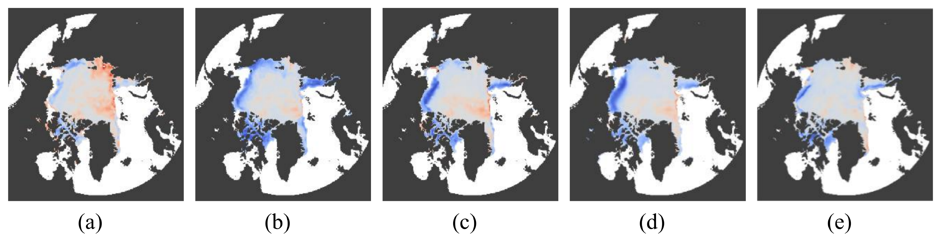
Figure 11 further compares the 14-day averaged spatial error distributions of SIC over the same test period. The GraphTransformer demonstrates lower overall error magnitude and a more spatially concentrated error pattern (Figure 11e), indicating enhanced capability in suppressing error dispersion. These results highlight the effectiveness of graph-structured spatial modeling in maintaining spatial coherence and improving prediction stability under complex Arctic ice conditions.

4.6.3. Quantitative Performance Comparison

Table 2. Comparison of 14-day averaged predictive performance of different models for Arctic sea ice thickness (SIT) and sea ice concentration (SIC) forecasting.

Model	${\overline{\mathbf{RMSE}}}_{\mathbf{SIT}}$ (m)	${\overline{\mathbf{MAE}}}_{\mathbf{SIT}}$ (m)	${\overline{{\mathit{R}}^2}}_{\mathbf{SIT}}$	${\overline{\mathbf{RMSE}}}_{\mathbf{SIC}}$	${\overline{\mathbf{MAE}}}_{\mathbf{SIC}}$	${\overline{{\mathit{R}}^2}}_{\mathbf{SIC}}$
GraphTransformer	0.2252	0.1531	0.8637	0.1019	0.0457	0.9487
GraphLSTM	0.2491	0.1769	0.8332	0.1402	0.0681	0.9029
ConvLSTM	0.2513	0.1851	0.8303	0.1423	0.0930	0.8999
PredRNN	0.2421	0.1744	0.8425	0.1286	0.0716	0.9183
U-Net	0.2231	0.1603	0.8599	0.1214	0.0543	0.9272

summarizes the 14-day averaged prediction performance of different models on the test set, including the root mean square error ($\overline{\mathrm{RMSE}}$), mean absolute error ($\overline{\mathrm{MAE}}$), and coefficient of determination ($\overline{R^2}$) for sea ice thickness (SIT) and sea ice concentration (SIC).

For the SIT forecasting task, GraphTransformer achieved an $\overline{\mathrm{RMSE}}$ of 0.2252 m, an $\overline{\mathrm{MAE}}$ of 0.1531 m, and an $\overline{R^2}$ of 0.8637 on the test set. Compared with GraphLSTM, the $\overline{\mathrm{RMSE}}$ and $\overline{\mathrm{MAE}}$ were reduced by 9.6% and 13.4%, respectively, indicating that the introduction of the Transformer module enhances the modeling of multi-step temporal dependencies under the same graph-structured spatial constraints. Relative to ConvLSTM, the $\overline{\mathrm{RMSE}}$ was further reduced by 10.4%.

While GraphTransformer demonstrates competitive performance in the SIT forecasting task, it does not consistently outperform U-Net in terms of $\overline{\mathrm{RMSE}}$ (Table 2). Specifically, U-Net achieves a slightly lower $\overline{\mathrm{RMSE}}$ of 0.2231 m for SIT forecasting, compared with 0.2252 m obtained by GraphTransformer (Table 2). Although the difference is modest (approximately 0.9%), this result indicates that convolutional architectures remain highly effective in capturing spatial patterns of sea ice thickness.

This relative weakness of GraphTransformer in highly localized regions may be related to differences in spatial modeling mechanisms. U-Net, as a fully convolutional architecture, benefits from the locality inductive bias of convolutional neural networks, which facilitates the extraction of fine-scale spatial features through hierarchical convolution and multi-scale skip connections [34]. Such properties are particularly advantageous for representing localized thickness gradients and detailed morphological structures in sea ice fields.

In contrast, the graph-structured mean aggregation strategy adopted in GraphTransformer emphasizes spatial-topological consistency across neighboring nodes. While neighborhood aggregation enhances large-scale structural coherence, repeated aggregation operations are known to potentially induce feature smoothing effects in graph neural networks [35]. This smoothing tendency may reduce sensitivity to highly localized spatial variability, especially in fragmented ice-edge regions.

For the SIC forecasting task, the superiority of GraphTransformer was more pronounced. It achieved an $\overline{\mathrm{RMSE}}$ of 0.1019, an $\overline{\mathrm{MAE}}$ of 0.0457, and an $\overline{R^2}$ of 0.9487. Compared with PredRNN, the $\overline{\mathrm{RMSE}}$ and $\overline{\mathrm{MAE}}$ were reduced by 20.8% and 36.2%, respectively, while $\overline{R^2}$ increased by approximately 0.03. Relative to U-Net, the $\overline{\mathrm{RMSE}}$ and $\overline{\mathrm{MAE}}$ were reduced by 16.1% and 15.8%, respectively. These results indicate that models relying solely on temporal modeling (PredRNN) or regular-grid convolution (U-Net) are less capable of accurately representing SIC evolution under complex spatial topological conditions. By explicitly incorporating graph-structured spatial constraints and leveraging the long-range temporal modeling capacity of the Transformer, GraphTransformer substantially improves multi-step SIC prediction accuracy and stability.

Overall, GraphTransformer achieved competitive and stable performance in the joint multi-step forecasting of SIT and SIC. In SIC prediction, it demonstrated clear advantages over PredRNN and U-Net, while in SIT prediction it maintained comparable accuracy to strong spatial baselines and further enhanced multi-step forecasting stability. These findings validate the effectiveness of integrating graph-structured spatial modeling with temporal Transformer mechanisms for Arctic sea ice prediction.

4.7. Temporal Evolution of Prediction Errors

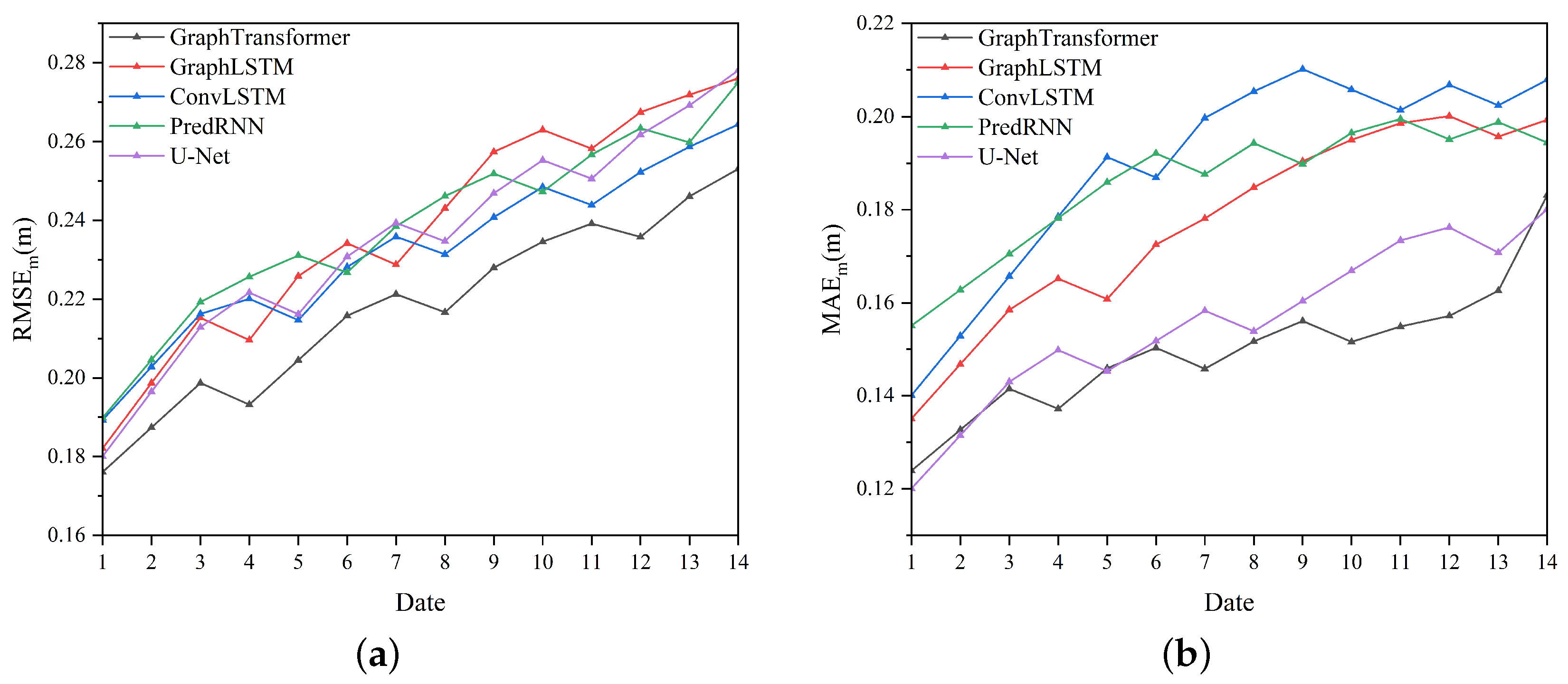
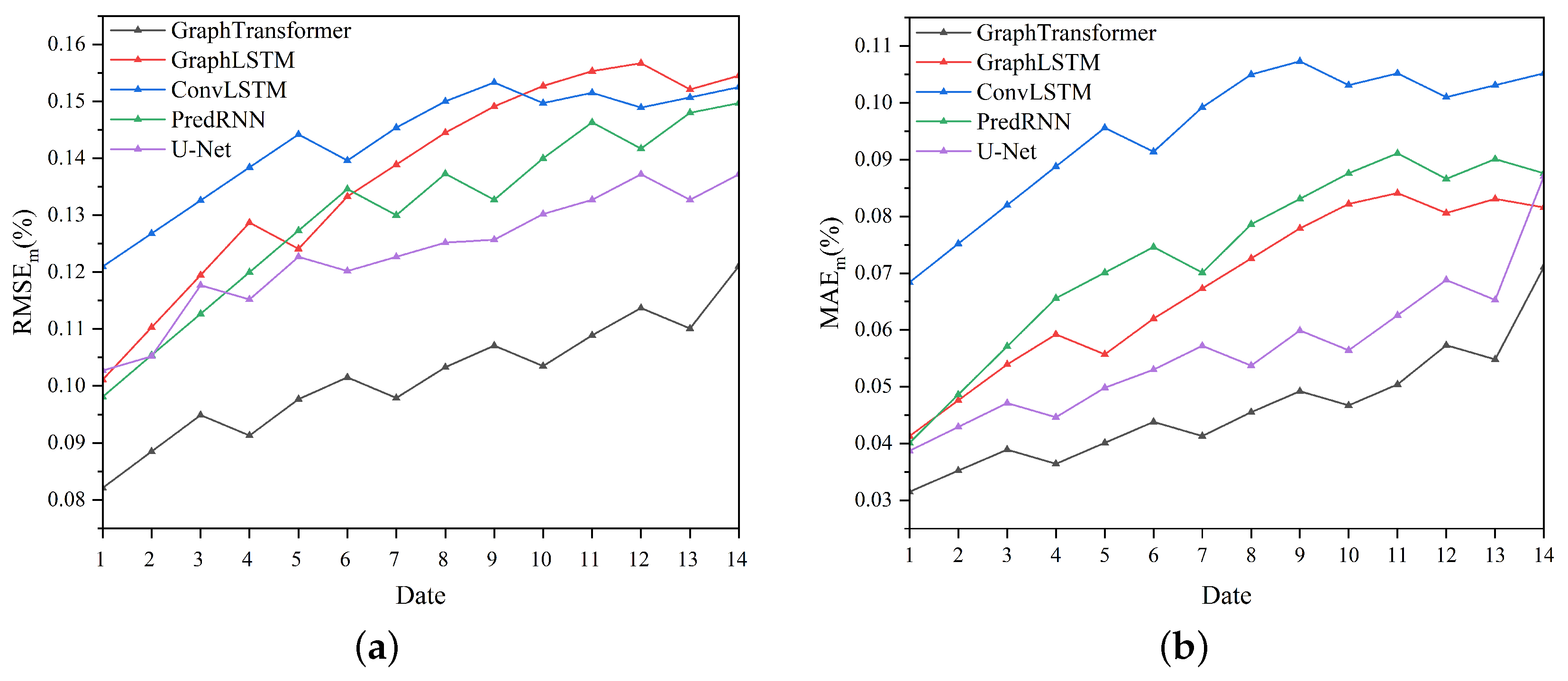
To further evaluate the stability of different models in multi-step forecasting, Figure 12 and Figure 13 illustrate the evolution of prediction errors for SIT and SIC on the test set as the forecast lead time increases.

In the multi-step SIT forecasting task (Figure 12), the prediction errors of all models exhibit a gradual increasing trend from Day 1 to Day 14, which is consistent with the progressive accumulation of forecasting uncertainty in sea ice thickness. In contrast, as shown in Figure 12a, GraphTransformer maintains a comparatively smooth error growth profile throughout the entire forecast horizon. Its ${\mathrm{RMSE}}_m$ is approximately 0.2213 m on Day 7 and 0.2531 m on Day 14, both of which are significantly lower than those of GraphLSTM and ConvLSTM. Although U-Net achieves error levels comparable to GraphTransformer during the short-range forecasting stage (e.g., Days 1–3), its error growth rate increases markedly as the forecast lead time extends, indicating weaker stability in longer-horizon predictions.

In the multi-step SIC forecasting task (Figure 13), performance disparities among different models become more pronounced. GraphTransformer consistently maintains the lowest prediction error throughout the entire 14-day forecast horizon. Specifically, its ${\mathrm{RMSE}}_m$ is approximately 0.0979 on Day 7 and 0.1211 on Day 14, indicating a relatively moderate error growth rate. In contrast, as shown in Figure 13a, the errors of PredRNN and U-Net accumulate more rapidly as the forecast lead time increases, resulting in noticeable deviations during the mid-to-late forecast stages. This suggests that models relying solely on temporal modeling or regular-grid convolution exhibit inherent limitations in capturing the long-term evolution characteristics of sea ice concentration.

Overall, GraphTransformer demonstrates superior stability in multi-step forecasting for both SIT and SIC. In particular, for the SIC task, it effectively suppresses the rapid amplification of prediction errors as the lead time extends. These findings indicate that incorporating graph-structured spatial constraints together with the long-range temporal modeling capability of the Transformer facilitates more robust multi-step forecasting under complex Arctic spatial topological conditions.

4.8. Ablation Study: Effect of Graph-Structured Spatial Modeling

To further verify the contribution of graph-structured spatial modeling within the GraphTransformer framework, an ablation experiment is conducted by introducing a pure Transformer model without graph structure as a baseline for comparison.

Figure 14 presents the spatial distribution results of the two models for both SIT and SIC prediction tasks. It can be observed that the pure Transformer exhibits evident spatial discontinuities and boundary blurring in certain regions.

In contrast, the incorporation of graph-structured spatial modeling in GraphTransformer substantially improves spatial coherence and continuity, effectively alleviating structural fragmentation in the predicted sea ice fields.

Table 3. Comparison of 14-day averaged predictive performance between GraphTransformer and the pure Transformer (without graph-structured spatial modeling) for Arctic sea ice thickness (SIT) and sea ice concentration (SIC) forecasting.

Model	${\overline{\mathbf{RMSE}}}_{\mathbf{SIT}}$ (m)	${\overline{\mathbf{MAE}}}_{\mathbf{SIT}}$ (m)	${\overline{{\mathit{R}}^2}}_{\mathbf{SIT}}$	${\overline{\mathbf{RMSE}}}_{\mathbf{SIC}}$	${\overline{\mathbf{MAE}}}_{\mathbf{SIC}}$	${\overline{{\mathit{R}}^2}}_{\mathbf{SIC}}$
GraphTransformer	0.2252	0.1531	0.8637	0.1019	0.0457	0.9487
Transformer	0.2362	0.1627	0.8620	0.1544	0.0786	0.8822

reports the 14-day averaged predictive performance of GraphTransformer and the pure Transformer (without graph-structured modeling) on the test set, providing a quantitative assessment of the contribution of graph-structured spatial modeling to the joint SIT–SIC forecasting task.

For the SIT prediction task, the pure Transformer achieves an $\overline{\mathrm{RMSE}}$ of 0.2362 m and an $\overline{\mathrm{MAE}}$ of 0.1627 m, representing relative increases of approximately 4.9% and 6.3%, respectively, compared with GraphTransformer. Meanwhile, its $\overline{R^2}$ shows a slight decrease.

In the SIC prediction task, the impact of graph-structured spatial modeling becomes more pronounced. The pure Transformer yields an $\overline{\mathrm{RMSE}}$ of 0.1544 and an $\overline{\mathrm{MAE}}$ of 0.0786, corresponding to increases of approximately 51.5% and 71.8%, respectively, relative to GraphTransformer. In addition, $\overline{R^2}$ decreases from 0.9487 to 0.8822.

These results demonstrate that incorporating graph-structured spatial constraints enhances spatial coherence in multi-step forecasting and mitigates cumulative error propagation. In particular, for SIC—whose spatial distribution is highly sensitive to structural topology—explicit modeling of neighborhood relationships plays a decisive role in improving multi-step prediction accuracy.

5. Limitations and Future Perspectives

Although the proposed GraphTransformer framework achieves competitive performance in the joint forecasting of sea ice thickness (SIT) and sea ice concentration (SIC) over the Arctic domain, several limitations should be acknowledged, which also motivate future research.

(1) Toward More Adaptive Spatial Graph Formulations: The spatial graph constructed in this study follows the four-neighbor (north–south–east–west) connectivity scheme defined in Section 2.2.1, where adjacency relationships are fixed on the native $0.25°$ latitude–longitude grid and represent geographical neighborhood rather than dynamic ice parcel trajectories. This static formulation preserves local topological consistency within the short-term 14-day prediction window and serves as a structural spatial constraint during training and inference. However, by construction, the graph does not explicitly model temporally evolving spatial dependencies induced by sea ice drift, deformation, or regime transitions. Although the underlying geographical topology remains stable over short horizons, the strength and directionality of physical interactions between grid cells may vary under different atmospheric–oceanic forcing conditions. Future research may therefore explore dynamic or adaptive adjacency mechanisms that retain geographical coherence while allowing interaction weights or connectivity patterns to evolve over time, thereby better characterizing time-varying spatial dependencies in Arctic sea ice systems [36,37].

(2) Toward Longer-Horizon Forecasting: The present study adopts a direct multi-step forecasting configuration with a fixed horizon of 14 days (from $t+1$ to $t+14$). While this setting aligns with the short-term operational forecasting objective and effectively mitigates recursive error accumulation, the model’s performance under longer forecast horizons has not been systematically evaluated. In particular, the stability of temporal attention mechanisms and graph-structured spatial constraints beyond the 14-day window remains unexplored. Future work may extend the forecasting horizon and investigate model robustness under longer-term prediction settings to further assess generalization capability and error growth behavior.

(3) Toward Deeper Integration of Physical Knowledge: While the proposed framework achieves stable joint forecasting performance for sea ice thickness (SIT) and sea ice concentration (SIC), the current modeling paradigm primarily relies on data-driven representation learning. The physical relationships governing Arctic sea ice evolution are reflected indirectly through historical observations rather than through explicitly formulated dynamical constraints. Future research may explore deeper integration of physically informed modeling strategies to enhance interpretability, structural consistency, and robustness under varying climatic regimes.

Future research may therefore explore dynamic adjacency mechanisms, extended temporal forecasting configurations, and physics-informed learning strategies to enhance the physical realism and generalization capability of graph-based Arctic sea ice prediction models.

6. Conclusions

This study addresses the joint forecasting problem of Arctic sea ice thickness (SIT) and sea ice concentration (SIC) over irregular spatial topologies. A GraphTransformer framework is proposed and validated, combining graph-structured spatial encoding with a temporal Transformer architecture. The main findings and contributions are summarized as follows:

(1) A GraphTransformer-based joint forecasting framework is developed. By explicitly modeling spatial neighborhood relationships on a static four-neighbor graph and integrating long-range temporal dependencies through the Transformer, the model achieves 14-day direct multi-step joint prediction of SIT and SIC.

(2) Comparative experiments based on multi-source daily observational and reanalysis data from 2019 to 2025 demonstrate that the proposed method achieves competitive overall performance for both SIT and SIC forecasting tasks, with particularly pronounced improvements in SIC prediction compared to multiple mainstream baseline models.

(3) Analysis of multi-step error evolution and ablation experiments further confirms that graph-structured spatial encoding plays a critical role in enhancing spatial coherence, mitigating error accumulation, and improving long-horizon forecasting stability. The results also indicate strong complementarity between graph-structured spatial modeling and Transformer-based temporal modeling.

Overall, the proposed GraphTransformer provides an effective and extensible data-driven framework for joint multi-step prediction of key Arctic sea ice variables, offering valuable technical support for high-latitude marine operations and climate-related research.